Quantum effects in biology: master equation studies of exciton motion in photosynthetic systems

Abstract

The present review is devoted to our recent studies on the excitonic motion in photosynthetic systems. In photosynthesis, the light photon is absorbed to create an exciton in the antenna complex of the photosynthetic pigments. This exciton then migrates along the chain-biomolecules, like FMO complex, to the reaction centre where it initiates the chemical reactions leading to biomass generation. Recently, it has been experimentally observed that the exciton motion is highly quantum mechanical in nature i.e., it involve long time ($\sim 600$ femto sec) quantum coherence effects. Traditional semiclassical theories like Forrester’s and second Born master equations cannot be applied. We point out why the 2nd Born non-Markovian master equation and its Markovian limit (also called the Redfield master equation) cannot be used to explain the observed long coherences. Briefly, the reason is that these approaches are perturbative in nature and in real light harvesting systems various couplings (system-system and system-bath) are of the similar order of magnitude. Various new approaches are being developed to go beyond the above two limiting theories. The present review is not a review in the usual sense of the word as we summarize our own approaches and only refer to the literature for the other ones. A brief introduction to the sophisticated 2D photon echo spectroscopy is also given at the end with an emphasis on the underlying physics of the multidimensional echo spectroscopies.

Key-words: Excitation energy transfer in photosynthesis; Quantum master equations; stochastic theories; line broadening; 2-D photon echo spectroscopy; Non-equilibrium statistical mechanics

I Introduction to Excitation Energy Transfer (EET) and the statement of the Problem

Photosynthesis provides chemical energy for almost all life on earth. Understanding of the natural photosynthesis can enable us to construct artificial photosynthesis devices and a solution to the future energy problems. We know that the safe (green) energy resources is a big challenge of the future and we know that our present energy technology is seriously disturbing our environmentmov . This prompts us to investigate “ Green” resources of energy and photosynthesis is one of them. Photosynthesis is an interesting phenomenon. On the average, on earth, biomass worth twice the mass of the Great Pyramid of Giza ($\sim 10$ million tons) is being produced every hour or $\sim 3$ million kg/sec.

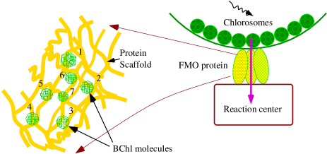
Figure 1: On the average, on earth, biomass worth twice the mass of the Great Pyramid of Giza ($\sim 10$ million tons) is being produced every hour. (Right) FMO protein acts as a “wire” which connects an antenna to a reaction center.

In photosynthetic systems a central role is played by the energy transport ”wire”–the FMO protein which is a trimer made of identical subunits containing seven bacteriochlorophyll (BChl) molecules each (Fig. 1). The photosynthesis process can be divided into the following stepsbooks1 :

1. A light photon is absorbed to create an excitation in the antenna complex of the photosynthetic pigments.

2. This excitation then migrates along the chain-biomolecules, like FMO complex, to the reaction center where it initiates the chemical reactions leading to biomass generation.

Quantum dynamics of EET (excitation energy transfer) can be very easily analyzed in the following two limiting cases. We identify first the couplings: Two important couplings:

1. Inter BChl molecules (system-system) coupling $J$ (which is responsible for EET).

2. The system-bath (BChl molecule-protein) coupling $\lambda$ (which is responsible for decoherence).

Two important timescales:

1. Excitation transfer time scale $\tau_{transfer}\equiv\frac{\hbar}{J}\sim 265fs,~{}~{}for~{}J\sim 20cm^{-1}\sim 4\times 10^{-22}joules$ (usual in photosynthesis pigments).

2. Decoherence time scale $\tau_{deco}\equiv\frac{\hbar}{\lambda}$.

If the system-bath coupling is very weak and $\tau_{deco}>>\tau_{transfer}$, the system is almost closed and dynamics is quantum mechanical in nature, i.e., one can use the Shroedinger’s equation to analyze it in the extreme case. But in the opposite case $\tau_{deco}<<\tau_{transfer}$ (strong system-bath coupling), the system is almost open, decoherence rate is very fast and the dynamics is almost incoherent. One can analyze the process with simple Pauli type master equation with rate of transfer of the excitation from one molecule to other calculated with Fermi’s golden rule (Forester’s theory)for .

Figure 2: Two extreme cases: (1) Upper: incoherent (classical diffusive motion), (2) Lower: ultra-quantum (delocalized excitation). The theoretical investigation of the intermediate case is a big challenge.

The important problem arises in the intermediate regime as real light harvesting systems do not fall in either of the extreme cases. Recently, it has been experimentally observed that the exciton motion is highly quantum mechanical in nature i.e., it involve long time ($\sim 600$ fs) quantum coherence effectsdis . These discoveries caused a lot of excitement in fieldexct as the traditional view was of incoherent ”hopping” of the exciton(Fig. 2). In the weak system-bath coupling case, the standard approach was the 2nd Born quantum master equation which is a perturbative quantum master equation (upto second order in system-bath interaction). Its Markovian and secular approximation is known as Redfield master equationbooks2 . The 2nd Born quantum master equation can be obtained from the Nakajima-Zwanzig projection operator technique by restricting the perturbation series upto second orderbooks2 . These simple and powerful projection operator techniques were introduced by Zawnzig in 1960’s in then active field of non-equilibrium statistical mechanics. As the the light harvesting pigments fall in the intermediate regime (system-bath coupling is of the order of system-system coupling) one clearly cannot use the 2nd order perturbative quantum master equation for its study in its original form. But in its modified form its scope becomes widergene .

It is of interest to quantitatively know upto what value of system-bath coupling strength and other important couplings in the problem, one can use the 2nd Born master equation. Section II deals with this.

In an important case of fast bath relaxation (when bath degrees-of-freedom re-organize very fast as compared to the transfer time scale of the exciton) a very useful approximation can be made. The details of which are given below. This is called the Markovian approximation. In the following sections we summarize our studynav of the quantitative determination of the regime of validity of the second order approximation and the Markovian approximation.

II Microscopic approach: 2nd Born master equation

As is well known that the 2nd Born quantum master equation can be obtained from the Nakajima-Zwanzig projection operator technique by restricting the perturbation series upto second order in the system-bath interactionbooks2 . In the following we will apply this master equation to a concrete model of a dimer (open two-state quantum system) which caricature the dynamics of decoherence in a typical photosynthetic systemif .

II.1 Non-Markovian solution

Projection super-operators and dynamics of the relevant system: The total system (relevant system (electronic part) + Bath (phonons)) dynamics is pure quantum in nature. The partial time derivative of the total density matrix is given by Liouville-van Neumann equation (classical equivalent is the invariance of the ”extension” in phase space):

$$\frac{\partial\hat{\rho}_{total}^{I}(t)}{\partial t}=\mathcal{L}(t)\hat{\rho}_{total}^{I}(t)\equiv-\frac{i}{\hbar}[H^{I}_{el-ph}+H_{b}^{I},\hat{\rho}_{total}^{I}(t)]$$ (1)

Here the interaction representation is used $\hat{O}^{I}(t)=U^{\dagger}_{S}(t)\hat{O}U_{S}(t),~{}~{}U_{S}(t)=Exp(-\frac{i}{\hbar}\hat{H}_{s}t)$ (see for details any standard refsbooks2 ). $H_{el-ph}$ is the system-bath interaction Hamiltonian (for the 2nd Born approximation $||H_{el-ph}||\ll||H_{s}||$. $H_{b}$ is the bath Hamiltonian. To construct the equation-of-motion for the relevant part of $\hat{\rho}_{total}^{I}(t)$ i.e., $\hat{\rho}(t)$, one defines the super-operator:

$$\mathcal{P}\hat{O}=\hat{R}_{eq}tr_{R}(\hat{O}),$$ (2)

called the projection super-operator, one also defines $\mathcal{Q}=I-\mathcal{P}$. By applying $\mathcal{P},~{}~{}\mathcal{Q}$ on the Liouville-van Neumann equation turn-by-turn, we get:

$$\frac{\partial\mathcal{P}\hat{\rho}_{total}^{I}(t)}{\partial t}=\mathcal{P}\mathcal{L}(t)(\mathcal{P}+\mathcal{Q})\hat{\rho}_{total}^{I}(t)$$

$$\frac{\partial\mathcal{Q}\hat{\rho}_{total}^{I}(t)}{\partial t}=\mathcal{Q}\mathcal{L}(t)(\mathcal{P}+\mathcal{Q})\hat{\rho}_{total}^{I}(t).$$ (3)

Solving the second equation formally for the irrelevant part $(\mathcal{Q}\hat{\rho}_{total}^{I}(t))$, and inserting in the first, one obtains the required equation-of-motion for the relevant part $(\hat{\rho}(t)\hat{R}_{eq}=\mathcal{P}\hat{\rho}_{total}^{I}(t))$ (see for detailsbooks2 ):

With 2nd Born approximation (i.e., by expanding the time evolution operator upto the first power in the system-bath interactionbooks2 ) and for a traditional dimer systemif :

$$H_{tot} = H_{s}+H^{ph}+H^{el-ph}$$

$$H_{s} = H^{el}+H^{reorg}$$

$$H^{el} = \sum_{n=1}^{2}\epsilon_{n}^{0}|n\rangle\langle n|+J(|1\rangle\langle 2|+|2\rangle\langle 1|)$$

$$H^{reog} = \sum_{n=1}^{2}\lambda_{n}|n\rangle\langle n|,~{}~{}~{}\lambda_{n}=\sum_{i}\hbar\omega_{i}d_{ni}^{2}/2$$

$$H^{ph} = \sum_{n=1}^{2}h_{n}^{ph},~{}~{}~{}~{}h_{n}^{ph}=\sum_{i}\hbar\omega_{i}(p_{i}^{2}+q_{i}^{2})/2$$

$$H^{el-ph} = \sum_{n=1}^{2}V_{n}u_{n},~{}~{}~{}~{}~{}~{}V_{n}=|n\rangle\langle n|,~{}~{}~{}u_{n}=-\sum_{i}\hbar\omega_{i}d_{ni}q_{i},$$ (4)

master equation takes the form,

$$\frac{\partial\rho^{I}(t)}{\partial t}=-\frac{i}{\hbar}\sum_{j=1}^{2}\langle u_{j}\rangle[V_{j}^{I},\rho^{I}]-$$

$$\frac{1}{\hbar^{2}}\sum_{i,j=1}^{2}\int_{0}^{t}d\tau(C_{ij}(t-\tau)[V_{i}^{I}(t),V_{J}^{I}(\tau)\rho^{I}(\tau)]-C_{ij}^{*}(t-\tau)[V_{i}^{I}(t),\rho^{I}(\tau)V_{J}^{I}(\tau)])$$ (5)

Here in the Hamiltonian, $|n\rangle$ represents the state in which ONLY $n$th site is excited and all others are in the ground state i.e., $|n\rangle=|\phi_{n,e}\rangle|\phi_{m\neq n,g}\rangle$. $H_{s}$ is the system Hamiltonian which consists of $H^{el}$ the electronic Hamiltonian for the two level system, and $H^{reorg}$ the Hamiltonian for the re-organization energy (the elastic energy related to the physical organization of the bath degrees-of-freedom). $H^{ph}$ is the phonon Hamiltonian and $H^{el-ph}$ is the system-bath coupling Hamiltonian. In the absence of phonons, $\epsilon_{n}^{0}$ is the excited electronic energy of $n^{th}$ site and $J$ is the electronic coupling between the sites which is responsible for excitation transfer. The ground state energies of both donor and acceptor are set equal to zero and $\lambda_{j}$ is the re-organization energy of the $j^{th}$ site (Dissipated energy in the bath after the electronic transition occurs). $d_{ji},q_{i},p_{i}$ are the dimensionless displacement of the equilibrium configuration of the $i^{th}$ phonon mode, dimensionless coordinates, momenta of the $i^{th}$ phonon mode respectively.

In the master equation, the bath correlation functions (bath is assumed to be a continuum of harmonic oscillators (valid when an-harmonic terms are not important)) are:

$$C_{ij}(t)\equiv\langle u_{i}(t)u_{j}(0)\rangle-\langle u_{i}\rangle\langle u_{j}\rangle$$ (6)

We consider a case where the characteristics of the bath as seen by both the sites are the same, and there is no systematic bath correlations between the sites. Thus the bath correlation function takes the form: $C_{ij}(t)=C(t)\delta_{ij}$:

$$C(t)=\int_{-\infty}^{+\infty}\frac{d\omega}{2\pi}C(\omega)e^{-i\omega t}.$$ (7)

$$C(\omega)=2\hbar(1+n(\omega))J(\omega),~{}~{}~{}~{}~{}J(\omega)=2\lambda\frac{\omega\gamma}{\omega^{2}+\gamma^{2}}$$ (8)

Assuming the Drude-Lorentz modelif for the bath spectral density, and assuming the high temperature approximation ($\frac{\hbar\omega}{k_{B}T}<<1$), as appropriate for the FMO problem, we obtain

$$C(t)=\frac{2\lambda}{\beta}e^{-\gamma t},~{}~{}~{}\beta=\frac{1}{k_{B}T}$$ (9)

II.2 Representations

The equation (5) is an operator equation and this can be expressed in site or in energy representation. In site representation, with definitions $x(t)\equiv\rho_{11}(t)\equiv\langle 1|\hat{\rho}(t)|1\rangle$ (site), $y_{1}(t)\equiv\textrm{Re}[\rho_{12}(t)]$, and $y_{2}(t)\equiv\textrm{Im}[\rho_{12}(t)]$, and with lengthy but straightforward calculations (see for detailsnav ), the equation (5) can be written explicitly as a set of coupled integro-differential delay equations:

$$\frac{dx(t)}{dt}= -2\frac{J}{\hbar}y_{2}(t)$$

$$\frac{dy_{1}(t)}{dt}= \frac{\Delta}{\hbar}y_{2}(t)-\frac{4\lambda}{\beta\hbar^{2}}e^{-\gamma t}\int_{0}^{t}d\tau e^{\gamma\tau}$$

$$\left[\eta_{1}\cos(E_{12}(t-\tau))y_{1}(\tau)+\eta_{2}\sin(E_{12}(t-\tau))y_{2}(\tau)\right]$$

$$\frac{dy_{2}(t)}{dt}= -\frac{\Delta}{\hbar}y_{1}(t)-\frac{J}{\hbar}(1-2x(t))-\frac{4\lambda}{\beta\hbar^{2}}e^{-\gamma t}\int_{0}^{t}d\tau e^{\gamma\tau}$$

$$\left[-\eta_{2}\sin(E_{12}(t-\tau))y_{1}(\tau)+\eta_{3}\cos(E_{12}(t-\tau))y_{2}(\tau)+2\Omega y_{2}(\tau)\right]$$

with $\eta_{1}=1,~{}~{}~{}\eta_{2}=-\frac{\Delta}{\sqrt{\Delta^{2}+4J^{2}}},~{}~{}~{}\eta_{3}=\frac{\Delta^{2}}{\Delta^{2}+4J^{2}},~{}~{}~{}~{}E_{12}=(E_{1}-E_{2})/\hbar=-\frac{\sqrt{\Delta^{2}+4J^{2}}}{\hbar},~{}~{}~{}\Omega=\frac{2J^{2}}{\Delta^{2}+4J^{2}}$.

For energy representation we need the eigensystem of the Hamiltonian. Let the kets $|e_{1,2}\rangle$ be the eigenstates of the Hamiltonian $H_{s}$. The reduced density matrix in energy representation can be expressed as:

$$\rho_{ab}^{e}(t)\equiv\langle e_{a}|\hat{\rho}(t)|e_{b}\rangle,$$ (10)

with time evolution given as,

$$\frac{d\rho_{ab}^{e}(t)}{dt}= -i\omega_{ab}\rho_{ab}^{e}-\frac{1}{\hbar^{2}}\sum_{i,c,d=1}^{2}\int_{0}^{t}d\tau C(t-\tau)$$ (11)

$$\left[V_{i}^{ac}V_{i}^{cd}e^{-i\omega_{cb}(t-\tau)}\rho_{db}^{e}(\tau)-V_{i}^{ac}V_{i}^{db}e^{-i\omega_{ad}(t-\tau)}\rho_{cd}^{e}(\tau)\right]$$

$$-C^{*}(t-\tau)\left[V_{i}^{ac}V_{i}^{db}e^{-i\omega_{cb}(t-\tau)}\rho_{cd}^{e}(\tau)-V_{i}^{cd}V_{i}^{db}e^{-i\omega_{ad}(t-\tau)}\rho_{ac}^{e}(\tau)\right],$$

with $\omega_{ab}=(E_{a}-E_{b})/\hbar$ and

$$V_{1}^{ac}=\frac{\alpha_{a}\alpha_{c}}{\sqrt{\alpha_{a}^{2}+1}\sqrt{\alpha_{c}^{2}+1}},~{}~{}~{}V_{2}^{ac}=\frac{1}{\sqrt{\alpha_{a}^{2}+1}\sqrt{\alpha_{c}^{2}+1}}.$$ (12)

Eigensystem of the Hamiltonian: Assuming $\lambda_{1}=\lambda_{2}\equiv\lambda$ the eigenvalues $E_{i}$ and eigenvectors $|e_{i}\rangle$ of the system Hamiltonian

$$H_{s}=\sum_{n=1}^{2}(\epsilon_{n}^{0}+\lambda_{n})|n\rangle\langle n|+J(|1\rangle\langle 2|+|2\rangle\langle 1|)$$

can be easily obtained as

$$E_{1,2}=\frac{1}{2}(\epsilon_{1}^{0}+\epsilon_{2}^{0}+2\lambda\mp\sqrt{(\epsilon_{1}^{0}+\epsilon_{2}^{0}+2\lambda)^{2}-4(\epsilon_{1}^{0}\epsilon_{2}^{0}-J^{2}+\lambda(\epsilon_{1}^{0}+\epsilon_{2}^{0})+\lambda^{2})})$$

$$|e_{1}\rangle=\frac{1}{\sqrt{\alpha_{1}^{2}+1}}\binom{\alpha_{1}}{1},~{}~{}~{}|e_{2}\rangle=\frac{1}{\sqrt{\alpha_{2}^{2}+1}}\binom{\alpha_{2}}{1}$$

$$\alpha_{1,2}=\frac{1}{2J}(\Delta\mp\sqrt{\Delta^{2}+4J^{2}}),~{}~{}~{}\Delta=\epsilon_{1}^{0}-\epsilon_{2}^{0}.$$

Here the column vectors denote components in the site basis. The eigenkets are normalized and are orthogonal $\alpha_{1}\alpha_{2}=-1$.

II.3 Numerical Approach

It is well known that the numerical propagation of integro-differential equations is an involved task and time consuming. In the following we construct a simple method to the solution of numerical integrationnav . Specifically we utilize the exponential nature of the bath correlation function which helps to convert the set of coupled integro-differential equations to a bigger set of ordinary differential equations:

$$f_{1}(t^{\prime})\equiv\int_{0}^{t^{\prime}}d\tau^{\prime}e^{\tau^{\prime}}\left[\cos[\frac{E_{12}}{\gamma}(t^{\prime}-\tau^{\prime})]\tilde{y}_{1}(\tau^{\prime})+\eta_{2}\sin[\frac{E_{12}}{\gamma}(t^{\prime}-\tau^{\prime})]\tilde{y}_{2}(\tau^{\prime})\right],$$

$$f_{2}(t^{\prime})\equiv\int_{0}^{t^{\prime}}e^{\tau^{\prime}}\tilde{y}_{2}(\tau^{\prime})d\tau^{\prime},$$

$$f_{3}(t^{\prime})\equiv\int_{0}^{t^{\prime}}d\tau^{\prime}e^{\tau^{\prime}}\left[-\eta_{2}\sin[\frac{E_{12}}{\gamma}(t^{\prime}-\tau^{\prime})]\tilde{y}_{1}(\tau^{\prime})+\eta_{3}\cos[\frac{E_{12}}{\gamma}(t^{\prime}-\tau^{\prime})]\tilde{y}_{2}(\tau^{\prime})\right].$$ (13)

With $t^{\prime}=\gamma t,~{}~{}\tau^{\prime}=\gamma\tau^{\prime}$. Here, $\tilde{y}_{1}(t^{\prime})\equiv y_{1}(t^{\prime}/\gamma),~{}~{}\tilde{y}_{2}(t^{\prime})\equiv y_{2}(t^{\prime}/\gamma)$ and we also define $\tilde{x}(t^{\prime})\equiv x(t^{\prime}/\gamma)$.

We obtain a set of coupled ordinary differential equations (note that these are much simpler to solve as compared to coupled integro-differential equations):

$$\dot{\tilde{x}}(t^{\prime})=-\frac{2J}{\gamma\hbar}\tilde{y}_{2}(t^{\prime}),$$

$$\dot{\tilde{y}}_{1}(t^{\prime})=\frac{\Delta}{\gamma\hbar}\tilde{y}_{2}(t^{\prime})-\frac{4\lambda}{\beta\gamma^{2}\hbar^{2}}e^{-t^{\prime}}f_{1}(t^{\prime}),$$

$$\dot{\tilde{y}}_{2}(t^{\prime})=-\frac{\Delta}{\gamma\hbar}\tilde{y}_{1}(t^{\prime})-\frac{J}{\gamma\hbar}+2\frac{J}{\gamma\hbar}\tilde{x}(t^{\prime})-\frac{8\lambda}{\beta\gamma^{2}\hbar^{2}}\Omega e^{-t^{\prime}}f_{2}(t^{\prime})-\frac{4\lambda}{\beta\gamma^{2}\hbar^{2}}e^{-t^{\prime}}f_{3}(t^{\prime}),$$

$$\ddot{f}_{1}(t^{\prime})-e^{t^{\prime}}\dot{\tilde{y}}_{1}(t^{\prime})=e^{t^{\prime}}\tilde{y}_{1}(t^{\prime})+\frac{E_{12}}{\gamma}e^{t^{\prime}}\eta_{2}\tilde{y}_{2}(t^{\prime})-\left(\frac{E_{12}}{\gamma}\right)^{2}f_{1}(t^{\prime}),$$

$$\dot{f}_{2}(t^{\prime})=e^{t}y_{2}(t),$$

$$\ddot{f}_{3}(t^{\prime})-e^{t^{\prime}}\eta_{3}\dot{\tilde{y}}_{2}(t^{\prime})=e^{t^{\prime}}\eta_{3}\tilde{y}_{2}(t^{\prime})-\frac{E_{12}}{\gamma}\eta_{2}{\gamma}e^{t^{\prime}}\tilde{y}_{1}(t^{\prime})-\left(\frac{E_{12}}{\gamma}\right)^{2}f_{3}(t^{\prime})~{},$$ (14)

Our aim is to use this to establish the parameter range over which the Markovian approximation is valid. Before doing so we compare this method with the traditional method of solution of integro-differential equationsvol . In the straightforward numerical method (traditional method) the integro-differential equation is first written as integral equation with double integration as $dx(t)/dt=\int_{0}^{t}f(x(t-\tau),t)d\tau$ converted to $x(t)=\int_{0}^{t}dt^{\prime}\int_{0}^{t^{\prime}}d\tau f(x(t^{\prime}-\tau),t^{\prime})$. The double integration is then done self-consistently with numerical integrationvol .

Speed: On the Lenovo ThinkCentre-i7, the traditional method took $\sim 15$ minutes to obtain the result, whereas the present method took only about a few milliseconds. A sample comparison is given in Fig. (3).

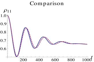
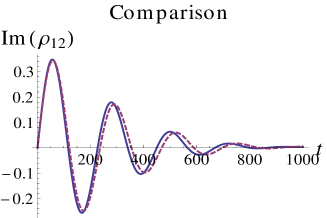
Figure 3: Comparison of numerical results for a traditional method (blue-solid curve), to that introduced here (red-dotted curve). Parameters used are: $\gamma=10^{13}~{}\textrm{s}^{-1},~{}~{}\lambda=2~{}\textrm{cm}^{-1},~{}~{}J=50~{}\textrm{cm}^{-1},~{}~{}\Delta=100~{}\textrm{cm}^{-1}$. Abscissa is in fs (fs $\equiv$ femto seconds).

II.4 Markovian limit

As mentioned before in an important case of fast bath relaxation (when bath degrees-of-freedom re-organize very fast as compared to the transfer time scale of the exciton) a very useful approximation can be made. This is called the Markovian approximationnote100 . To do this approximation, note that it is particularly simple to invoke it in the energy representation (as one can “average out” the fast oscillations in the system’s density matrix and can compare the temporal envelope of the system’s density matrix with time decay of the bath correlation function). Hence, below we first utilize the energy basis and then convert the result back to the site representation.

The Markov approximation can be performed when the time scale on which the envelope of the density matrix decays is much longer than the decay time of the phonon correlation function books2 . One can then introduce the following approximation:

$$\rho_{ab}^{e}(t-\tau)\equiv e^{-i\omega_{ab}(t-\tau)}\tilde{\rho}_{ab}^{e}(t-\tau)\simeq e^{-i\omega_{ab}(t-\tau)}\tilde{\rho}_{ab}^{e}(t)=e^{i\omega_{ab}\tau}\rho_{ab}^{e}(t).$$

To do this energy representation equations are first converted to dimensionless form with $\tau^{\prime}=\gamma\tau$ (see for detailsnav ). Putting $t-\tau=\tau^{\prime}$ in the resulting equations and then implementing the above approximation on the density matrix elements allows the time integration to be performed easily for the case of exponential phonon correlation function. The result is the set of Markovian equations:

$$\dot{\tilde{\rho}}_{ab}^{e}(t^{\prime})=-i\bar{\omega}_{ab}\tilde{\rho}_{ab}^{e}(t^{\prime})$$

$$-\frac{2\lambda}{\beta\hbar^{2}\gamma^{2}}\sum_{i,c,d}\left(\frac{V_{i}^{ac}V_{i}^{cd}}{1-i\bar{\omega}_{dc}}\tilde{\rho}_{db}^{e}(t^{\prime})-\frac{V_{i}^{ac}V_{i}^{db}}{1+i\bar{\omega}_{db}}\tilde{\rho}_{cd}^{e}(t^{\prime})\right)$$

$$+\frac{2\lambda}{\beta\hbar^{2}\gamma^{2}}\sum_{i,c,d}\left(\frac{V_{i}^{ac}V_{i}^{db}}{1-i\bar{\omega}_{ca}}\tilde{\rho}_{cd}^{e}(t^{\prime})-\frac{V_{i}^{cd}V_{i}^{db}}{1+i\bar{\omega}_{cd}}\tilde{\rho}_{ac}^{e}(t^{\prime})\right).$$

Here $\rho^{e}_{ab}(t^{\prime}/\gamma)\equiv\tilde{\rho}^{e}_{ab}(t^{\prime}),~{}~{}\bar{\omega}_{ab}\equiv\omega_{ab}/\gamma$. The results can then be transformed back to the site representation using $\rho_{ij}(t)=\langle i|{\rho}(t)|j\rangle=\sum_{a,b}\langle i|e_{a}\rangle\rho_{ab}^{e}\langle e_{b}|j\rangle$.

II.5 Limiting Cases: Analytical Results

Markovian and non-Markovian results were obtained computationally and compared for various regimes. Before presenting them we show some interesting analytic results in two extreme cases on the parameter dependence of the region of validity of the Markov approximation:

II.5.1 Strong Coupling Case: $J\gg\Delta$

For $J\gg\Delta$, we have $\alpha_{1}\simeq 1,~{}~{}\alpha_{2}\simeq-1,$ and $V_{1}^{ij}\simeq 1/2$ for $i=j$ and $\simeq-1/2$ for $i\neq j~{}~{}(\{i,j\}=1,2)$ and $V_{2}^{i,j}\simeq 1/2$ for all $i,j$. One can then analytically solve the coupled equations to obtain the simple expression

$$\tilde{\rho}_{11}^{e}(t^{\prime})=\frac{1}{2}(e^{-\frac{4\lambda}{\beta(4J^{2}+\hbar^{2}\gamma^{2})}t^{\prime}}+1),$$ (15)

for the traditional initial conditions $\tilde{\rho}_{11}^{e}(t^{\prime}=0)=1,~{}~{}\tilde{\rho}_{12}^{e}(t^{\prime}=0)=\tilde{\rho}_{21}^{e}(t^{\prime}=0)=0$. The Markov approximation can be performed when the time scale on which the envelope of the density matrix decays is much longer than the decay time of the phonon auto-correlation function. Hence, $\boxed{\frac{4\lambda}{\beta(4J^{2}+\hbar^{2}\gamma^{2})}\ll 1}$ must hold for the Markov approximation to be valid in the $J\gg\Delta$ domain.

II.5.2 Weak Coupling Case: $J\ll\Delta$

For this case, we have $\alpha_{1,2}=\frac{1}{2J}(\Delta\mp\sqrt{\Delta^{2}+4J^{2}})\simeq\frac{\Delta}{2J}(1\mp 1)$. Hence, in this domain $\alpha_{1}\simeq 0$, and $\alpha_{2}\simeq\Delta/J$. This leads to $V_{1}^{11}=V_{1}^{12}=V_{1}^{21}\simeq 0,~{}~{}V_{1}^{22}\simeq 1$. $V_{2}^{11}\simeq 1,~{}~{}V_{2}^{12}=V_{2}^{21}\simeq J/\Delta$, and $V_{2}^{22}=(J/\Delta)^{2}$.

$$\dot{\tilde{\rho}}_{11}^{e}(t^{\prime})=$$

$$\frac{2/\lambda}{\hbar^{2}\beta\gamma^{2}}\left(2(J/\Delta)^{2}(\Gamma+\Gamma^{\ast})-4(J/\Delta)^{2}(\Gamma+\Gamma^{\ast})\tilde{\rho}_{11}^{e}(t^{\prime})+2(J/\Delta)(\tilde{\rho}_{12}^{e}(t^{\prime})+\tilde{\rho}_{21}^{e}(t^{\prime}))\right),$$

$$\dot{\tilde{\rho}}_{12}^{e}(t^{\prime})=\frac{i\Delta}{\hbar\gamma}\tilde{\rho}_{12}^{e}(t^{\prime})+$$

$$+\frac{4\lambda}{\hbar^{2}\beta\gamma^{2}}\left((J/\Delta)\Gamma^{\ast}(2\tilde{\rho}_{11}^{e}(t^{\prime})-1)-(1+2\Gamma(J/\Delta)^{2})\tilde{\rho}_{12}^{e}(t^{\prime})+2(J/\Delta)^{2}\Gamma^{\ast}\tilde{\rho}_{21}^{e}(t^{\prime})\right).$$

where $\Gamma=\frac{1}{1+i\frac{\Delta}{\hbar\gamma}}$. See for details the second paper innav . By separating real and imaginary parts as $\tilde{\rho}_{12}^{e}(t^{\prime})=x(t^{\prime})+iy(t^{\prime})$ and writing $\tilde{\rho}_{11}^{e}(t^{\prime})=r(t^{\prime})$, we have:

$$r(t^{\prime})=\frac{1}{\eta^{2}+\xi^{2}}(\eta^{2}+\xi^{2}+[a\xi-b\eta]\epsilon\xi$$

$$[b\eta-a\xi]\epsilon\xi\cos(\eta t^{\prime})e^{-\xi t^{\prime}}+[a\eta+b\xi]\epsilon\xi\sin(\eta t^{\prime})e^{-\xi t^{\prime}}),$$

$$x(t^{\prime})=e^{-\xi t^{\prime}}(a\cos(\eta t^{\prime})-b\sin(\eta t^{\prime})),$$

$$y(t^{\prime})=e^{-\xi t^{\prime}}(a\sin(\eta t^{\prime})+b\cos(\eta t^{\prime})).$$ (16)

with initial conditions $r(t^{\prime}=0)=1,~{}~{}x(t^{\prime}=0)=a,~{}~{}y(t^{\prime}=0)=b$. Here $\xi={4\lambda}/(\hbar^{2}\beta\gamma^{2}),~{}~{}\eta={\Delta}/{\hbar\gamma},$ and $\epsilon={J}/{\Delta}$. Thus, for the Markov approximation to hold requires $\boxed{\xi=4\lambda/\beta\hbar^{2}\gamma^{2}\ll 1}$. These are summarized in Table 1. A numerical verification of these analytical inequalities is given in Fig. (4).

Table 1: Regimes of validity of the Markov approximation

Case	Markovian approximation
$J>>\Delta$	$\frac{4\lambda}{\beta(4J^{2}+\hbar^{2}\gamma^{2})}<<1$
$J<<\Delta$	$\frac{4\lambda}{\hbar^{2}\beta\gamma^{2}}<<1$

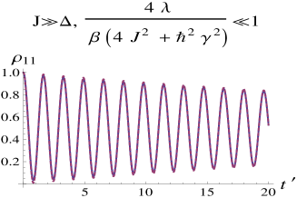
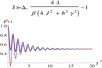
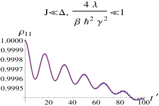
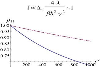
Figure 4: Sample verification of the analytic inequalities (Table I). Time evolution of population on site 1: blue (solid) curve is the non-Markovian solution and red (dotted) curve is the Markovian approximation.

II.6 Computational Results

To investigated the validity regime of Markovian approximation beyond the above two limiting cases we have to rely on the numerical computation (as the analytic approach becomes very cumbersome). We here display an extensive list of graphs (Figs. 5,6, and 7) which explore how Markovian approximation behaves for various values of parameters.

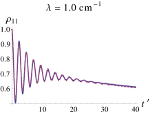
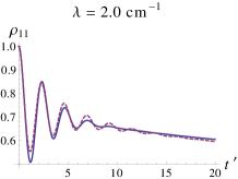
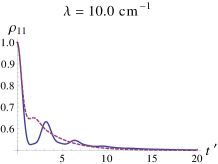
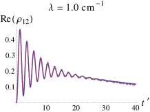
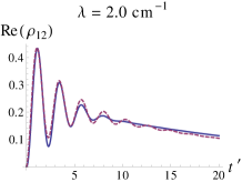
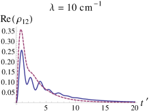
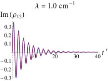
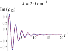
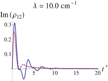
Figure 5: Time evolution of population on site 1 [$\rho_{11}(t)$] and the coherences [$\rho_{12}(t)$] [blue (solid) curve is the non-Markovian solution and red (dotted) curve is the Markovian approximation], for various values of $\lambda$ (in cm^-1). Other parameter are: $\Delta$ = 100 cm^-1, $J$ = 50 cm^-1,  $\gamma=10^{13}$ s^-1.

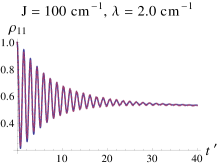
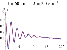
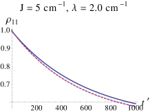
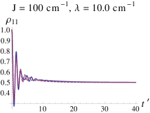
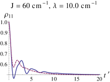
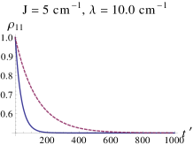
Figure 6: Time evolution of population on site 1: blue (solid) curve is the non-Markovian and red (dotted) curve is the Markovian) for various values of the reorganization energy $\lambda$ and inter-site coupling $J$.

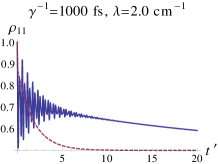
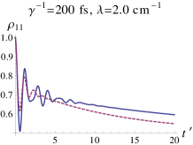
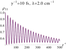
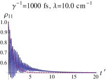
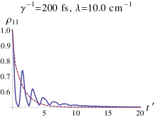
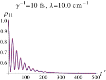
Figure 7: Time evolution of population on site 1 [blue (solid) curve is the non-Markovian and red (dotted) curve is the Markovian] for various values of the reorganization energy $\lambda$ and phonon relaxation time $\gamma^{-1}$.

First consider the non-Markovian results (solid curves). Coherent oscillatory dynamics up to substantial time scales are evident. Oscillatory behavior in the populations are seen (Fig. 5) to be accompanied by oscillations in the off diagonal elements $\rho_{12}$ representing coherences. The oscillations fall off faster with increasing re-organization energies, as expected. Another point to be noted is that the relaxation to equilibrium populations occurs on a longer time scale than does relaxation of the coherences to zero. This difference is more evident at smaller values of re-organization energy $\lambda$. The dependence of population relaxation on the bath correlation decay time $\gamma^{-1}$ is shown in Fig. 7. Clearly, the larger the $\gamma$ (i.e., fast bath relaxation), the better is the Markov approximation.

Figures 5 - 7 also contain a comparison of the Markovian limit to the non-Markovian solution for domains other than those in Table I. For the standard electronic coupling parameter values in photosynthetic EET: $\gamma^{-1}=100~{}\textrm{fs},~{}~{}J=50~{}\textrm{cm}^{-1},~{}~{}\Delta=100~{}\textrm{cm}^{-1},~{}~{}T=300~{}$K, figure 5 shows that the Markovian approx is very good for $\lambda=1~{}\textrm{cm}^{-1}$, fair for $\lambda=2~{}\textrm{cm}^{-1}$, and invalid for reorganization energies $\lambda\geq 10~{}\textrm{cm}^{-1}$. As typical values of $\lambda$ in photosynthetic EET systems are considerably larger than $\lambda=10$ cm^-1, these results support the conclusions of Ref. if , although with a different approach.

Figs. 6 and 7 show the validity of the Markov approximation obtained by varying $(J,\lambda)$ and $(\gamma^{-1},\lambda)$ respectively, but keeping $\Delta=100$ cm^-1. The results show that the Markovian approximation is poor for large $\lambda$ and small $J$, and for large $\gamma^{-1}$ and small $\lambda$. Other parameter values can be easily examined using this approach.

From these qualitative conclusions a rough physical picture can be drawn as depicted in Fig. (8). In the Markovian regime, after photo-excitation, bath (nuclear co-ordinates) re-organize very fast representing an ”apt” bath (right hand picture) while in the non-Markovian regime bath correlations exist for longer time scale (of the order of exciton transfer time scale). Thus the combined (system+bath) dynamics is much more complicated in the non-Markovian regime.

Figure 8: Approximate Physical Picture

Here, results are given for the particular initial conditions: $\rho_{11}(0)=\tilde{x}(0)=1,~{}~{}\tilde{y}_{1}(0)=\tilde{y}_{2}(0)=0,~{}~{}f_{1}(0)=f_{2}(0)=f_{3}(0)=\dot{f}_{1}(0)\dot{f}_{3}(0)=0$. These initial conditions (corresponding to all the population being on site 1, and no coherences) are those which have been used extensively in literatureif but are somewhat unphysicalif3 , because they lack initial coherences which become important in preparatory photo-excitation. We have considered this problem in the second reference of the listnav which considers photo-excitation of a dimer oscillator system with an ultra-short laser pulse. It appeared that the presence of initial coherence ( at $t^{\prime}=0$) effected the time scale on which the populations reach equilibrium value but had little effect on the overall damping-out of the coherences (see for detailsnav ).

III Phenomenological approach: a stochastic model

In the previous sections we saw that 2nd Born quantum master equation cannot be applied to the real light harvesting systems as in these systems the system-bath coupling ($\lambda\sim 100~{}cm^{-1}$) is of the same order of magnitude of the system-system coupling ($J\sim 100~{}cm^{-1}$). To make the situation more intractable, it is not possible to justify the Markovian approximation when $\lambda\gg 1~{}cm^{-1}$ (given that Markovian master equations are much easier to solve than the non-Markovian ones). Thus the use of Markovian Redfield theory to these systems is questionable as pointed out inif ; nav . This open up a difficult problem. One should formulate some non-perturbative theories. Recently Ishizaki and Flemingif have developed a formalism which goes beyond the limitations of the 2nd Born master equation. They use the reduced hierarchy equation approach previously developed by Tanimura and Kubotk . There is an other route to the problem pioneered by people like Silbeysilbey . In this approach one uses a unitary transformation (called polaron transformation) to completely eliminate the system-bath coupling Hamiltonian. But this re-normalize the system Hamiltonian. Then one re-partition the resulting system Hamiltonian to identify a weaker term which can be used as a perturbation. The remaining problem is done in line with 2nd Born master equationjang .

We have developed an alternative stochastic approach which is phenomenological in naturenav3 . This approach, as its input, takes the homogeneous line width from the experiment and uses Kubo’s stochastic theory of motional narrowing to get phenomenological decoherence rate.

III.1 The model and its solution

We again consider the dynamics of exciton transfer between two molecules modeled as two-level electronic systems (Fig. 9). These two-level systems are electronically coupled with each other with coupling $J$.

Figure 9: Two interacting molecules

Due to the electronic coupling between the molecules the exciton will transfer back-and-forth between the molecules. This will happen forever if the molecules are completely isolated—pure oscillatory quantum motion. Now consider that our two-molecular system is open i.e., interacting with the external bath degrees-of-freedom—-the phonons. It is well known that the dynamics remain quantum at short time scales and becomes classical at longer time scalesrush . This quantum-to-classical crossover happens at a critical time scale which is inversely proportional to system-bath coupling energy ($t_{c}\propto\frac{\hbar}{\eta}$). Large $\eta$ (system-bath coupling) means fast quantum-to-classical crossover and vice versa. We denote system-bath coupling strength with $\eta$ in the subsequent subsections (before we used $\lambda$).

In a recent contributionnav3 we extracted $\eta$ from experimental information using Kubo’s stochastic theory of line shapes and observed upto what timescale one could see quantum effects.

The important point is that we modeled the dynamical effect of phonons as a stochastic noise. The total Hamiltonian takes the form

$$H=\epsilon_{1}|1\rangle\langle 1|+(\epsilon_{2}+\epsilon(t))|2\rangle\langle 2|+J(|1\rangle\langle 2|+|2\rangle\langle 1|).$$ (17)

Here $\epsilon_{1}$ is the energy of the upper electronic level of the first molecule and $\epsilon_{2}$ is that of the second molecule. The ground state energies of both the molecules are taken to be zero. The energy separation $\epsilon_{2}-\epsilon_{1}$ has a random component (due to phonons) which we denote with $\epsilon(t)$. $\epsilon(t)$ is a stochastic process taken here as Gaussian White Noise (GWN):

$$\langle\epsilon(t)\rangle=0,~{}~{}~{}\langle\epsilon(t)\epsilon(\tau)\rangle=\hbar^{2}\eta\delta(t-\tau).$$ (18)

Here, as mentioned before, $\eta$ is the strength of system-bath coupling (also known as dynamical disorder) measured in the units of frequency.

We start with Liouville-von-Neumann equation for the total density matrix,

$$i\hbar\frac{\partial\hat{\rho}(t)}{\partial t}=[\hat{H},\hat{\rho}(t)].$$ (19)

As $\hat{H}$ is a stochastic operator, thus $\hat{\rho}(t)$ is also a stochastic operator. Therefore, we need to evaluate the averaged density matrix. So we need to do an averaging over the dynamical disorder which is denoted by $\langle...\rangle$. We define $\varsigma(t)\equiv\langle\rho(t)\rangle$.

Averaging over dynamical disorder:

$$i\hbar\frac{d\varsigma(t)}{dt}=\underbrace{\langle H\rho(t)\rangle}_{TermI}-\underbrace{\langle\rho(t)H\rangle}_{TermII}.$$ (20)

In term I and II above we have terms like $\langle\rho(t)\epsilon(t)\rangle$. As $\rho(t)$ is a functional of $\epsilon(t)$ (a stochastic quantity) the $\rho(t)$ will also be a stochastic function. To decouple these we will use the famous theorem of Novikovnovi :

$$\langle\epsilon(t)\rho_{ab}(t)\rangle=\int_{-\infty}^{\infty}dt^{\prime}\langle\epsilon(t)\epsilon(t^{\prime})\rangle\left\langle\frac{\delta\rho_{ab}(t)}{\delta\epsilon(t^{\prime})}\right\rangle$$ (21)

Here $\frac{\delta\rho_{ab}(t)}{\delta\epsilon(t^{\prime})}$ is the functional derivative. Using the properties of stochastic noise and with some simplification(see appendix A), we get

$$\langle\epsilon(t)\rho_{12}(t)\rangle=i\hbar\eta\varsigma_{12}(t).$$ (22)

Finally, one has a set of coupled differential equations:

$$\frac{d\varsigma_{11}(t)}{dt}=-i(J/\hbar)(\varsigma_{21}(t)-\varsigma_{12}(t))$$

$$\frac{d\varsigma_{12}(t)}{dt}=-i(\Delta/\hbar)\varsigma_{12}(t)-i(J/\hbar)(\varsigma_{22}(t)-\varsigma_{11}(t))-\eta\varsigma_{12}(t)$$

$$\varsigma_{11}(t)+\varsigma_{22}(t)=1.$$ (23)

The above system of ODEs can be solved analytically, however, the exact expression is very cumbersome. We give the analytic solution only in the long time limit (see Appendix B).

To simulate the dynamics of decoherence in this dimer model with physical parameters of the FMO problem ($\Delta=\epsilon_{1}-\epsilon_{2}\simeq 100cm^{-1},~{}J\simeq 100cm^{-1}$), we need to find out our phenomenological parameter $\eta$, for this we use Kubo’s stochastic theory of lineshapes.

III.2 Kubo’s stochastic theory of lineshapes and estimation of $\eta$ from motionally narrowed lineshape

We now determine the phenomenological parameter $\eta$. Let us focus on exciton 1 in 2-D photon echo spectra which occurs at $810~{}nm$ (Fig. 10).

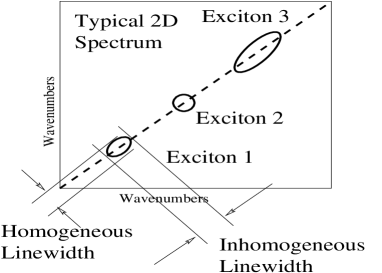
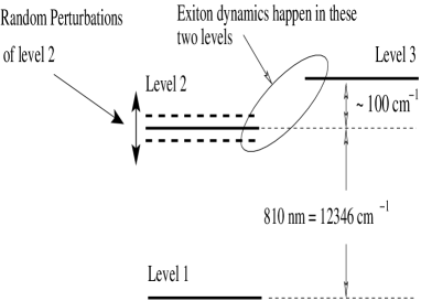
Figure 10: (Left) Schematic line broadening information in 2-D photon echo spectrum shown without cross peaks. The linewidth due to homogeneous and in-homogeneous broadening are in orthogonal directions as shown. (Right) The energy levels of the model system

We use Kubo’s randomly modulated oscillator model for the exciton under question. The energy levels of the model system are given in Fig. 10. The levels 1 and 2 are separated on the average by $\omega_{0}=810~{}nm$.

Let the level 2 be randomly modulated with a random process $\omega_{1}(t)$ such that $\lim_{T\rightarrow\infty}\frac{1}{T}\int_{0}^{T}\omega_{1}(t)dt=0$. The random frequency of the level 2 is then given as $\omega(t)=\omega_{0}+\omega_{1}(t)$. We use the classical oscillator model for the molecule with resonance frequency $\omega_{0}=810~{}nm$. The equation of motion is $\dot{x}(t)=i\omega(t)x(t)$, with solution

$$x(t)=x(0)\exp{\left(i\omega_{0}t+i\int_{0}^{t}\omega_{1}(t^{\prime})dt^{\prime}\right)}.$$ (24)

The absorption spectrum measures a large number of possible realizations of the random process $\omega_{1}(t)$ ( The radiation field acts on a macroscopic number of molecules present with different realizations of $\omega_{1}(t)$ in the sample). Thus one need to consider an ensemble average to compare with absorption spectrum:

$$\langle x(t)\rangle=x(0)e^{i\omega_{0}t}\left\langle\exp{\left(i\int_{0}^{t}\omega_{1}(t^{\prime})dt^{\prime}\right)}\right\rangle,$$ (25)

and the average time correlation is given by $\langle x(t)x^{\ast}(0)\rangle=|x(0)|^{2}e^{i\omega_{0}t}\phi(t)$ where

$$\phi(t)=\left\langle\exp{\left(i\int_{0}^{t}\omega_{1}(t^{\prime})dt^{\prime}\right)}\right\rangle$$ (26)

is called the relaxation function of the oscillator. The absorption spectrum is

$$I(\omega-\omega_{0})=\frac{1}{2\pi}\int_{-\infty}^{+\infty}e^{-i(\omega-\omega_{0})t}\phi(t)dt.$$ (27)

This is the direct consequence of the famous fluctuation-dissipation theorem. The temporal character of the decay of fluctuations tells directly the dissipative characteristics of the system. The intensity distribution $I(\omega)$ will be broadened by the stochastic process $\omega_{1}(t)$. To define the stochastic process $\omega_{1}(t)$ let $P(\omega_{1})d\omega_{1}$ be the probability to find the random frequency $\omega_{1}$ to be in the range $\omega_{1}$ to $\omega_{1}+d\omega_{1}$ when picked randomly from the ensemble. In Kubo’s theory, the stochastic process is defined with two parameters (1) magnitude of modulation $\Delta^{2}=\int\omega_{1}^{2}P(\omega_{1})d\omega_{1}=\langle\omega_{1}^{2}\rangle$ and (2) correlation time $\tau_{c}=\int_{0}^{\infty}f_{c}(t)dt$ where correlation function is defined as $f_{c}(\tau)=\frac{1}{\Delta^{2}}\langle\omega_{1}(t)\omega_{1}(t+\tau)\rangle$.

It is well known that for a Gaussian process, relaxation function can be written in terms of the correlation function:

$$\phi(t)=\exp{\left(-\Delta^{2}\int_{0}^{t}(t-\tau)f_{c}(\tau)d\tau\right)}$$ (28)

In the present case we have considered Gaussian White Noise (GWN) which has zero correlation time. Our case corresponds to the fast modulation case of Kubo $\tau_{c}<<\frac{1}{\Delta}$sto . The correlation function decays very fast and the upper limit of the integral in the above equation can be extended to $\infty$. This leads to $\phi(t)\propto e^{-\Delta^{2}\tau_{c}|t|}$. This results in the famous narrowing of the lineshape from the Gaussian to Lorentzian form. In the present case we have $\langle\frac{\epsilon(t)}{\hbar}\frac{\epsilon(t+\tau)}{\hbar}\rangle=\eta\delta(\tau)$ which leads to $\phi(t)=e^{-\eta|t|}$. Comparison with the previous $\phi(t)$ shows that $\eta=\Delta^{2}\tau_{c}$ which gives the rate of decay of the correlation function. In our GWN case $\Delta\rightarrow\infty$ since white noise contains all frequencies and $\tau_{c}\rightarrow 0$ (delta correlated noise) but $\Delta^{2}\tau_{c}$ is finite and is equal to $\eta$.

Thus the absorption spectrum takes the form

$$I(\omega-\omega_{0})=\frac{1}{\pi}\frac{\eta}{(\omega-\omega_{0})^{2}+\eta^{2}}.$$ (29)

This is the famous Lorentzian lineshape narrowed from the Gaussian shape (called motional narrowing).

Our aim is to find out our phenomenological parameter $\eta$. Thus we need to fit this $I(\omega-\omega_{0})$ with the real experimental observation and to extract $\eta$. We will use this to simulate the quantum dynamics of the density matrix elements.

The basic problem with linear absorption line shape is that it is broadened both by homogeneous and in-homogeneous mechanisms. In our case the broadening is homogeneous due to dynamical disorder and thus we need to subtract the in-homogeneous component due to static disorder. But thanks to the 2-D photon echo spectroscopy one has the important information about both homogeneous and in-homogeneous broadening (see Fig. 10). A brief introduction to the physics of 2D photon echo spectroscopy is given in the appendix c (for details see for example2dphoton ). We want to measure Full Width at Half Maximum (FWHM) of the homogeneously broadened peaknote1 . We consider Fig 2 (a) of G. S. Engel et. algs . The homogeneous broadening is along the main diagonal (see Fig. 10). From the scale given in terms of nano-meters of the figure 2(a) of G. S. Engel et. al., the FWHM is about $\simeq 10nm$ and the exciton peak occurs at $810~{}nm$. This gives the frequency broadening $\delta\omega_{FWHM}\simeq 2.87\times 10^{13}Hz$.

With this experimental information we plot $I(\omega-\omega_{0})$ such that FWHM is about $\simeq 10nm=2.8710^{13}Hz$. Clearly for the Lorentzian, at FWHM $\delta\omega_{FWHM}=2\eta$. This gives $\eta=0.0143~{}fsec^{-1}$.

III.3 Long coherences

We now have all the required parameters, from the experimental information, namely, $\eta=0.0143~{}fsec^{-1},~{}J=100cm^{-1},~{}{\rm and}~{}\Delta=100cm^{-1}$. With these values we plot the dynamics of the density matrix elements $r(t),~{}x(t),~{}{\rm and}~{}y(t)$. We clearly see that the density matrix elements show oscillations upto $500fsec$, mimicking the long coherences observed in the experiments of G. S. Engel et. al. To reproduce the actual spectra observed for example by G. S. Engel et. al. one has to go beyond this simple two state model. One has to consider a detailed model of the FMO complex containing not the two coupled molecules (as considered here) but the seven coupled BChl molecules and there interactions with the protein matrix. This clearly requires a considerable computational challenge and one has to rely on the numerical approach rather than on an simple analytical solution as given here.

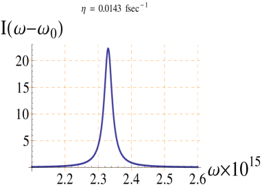
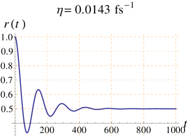
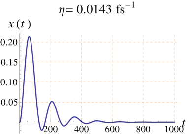
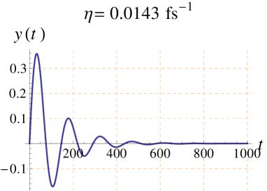
Figure 11: Line shape function $I(\omega)$ for $\Delta=100cm^{-1},J=100cm^{-1},~{}~{}\eta=0.0143~{}fsec^{-1}$ (upper left). This value of $\eta$ i.e., $0.0143~{}fsec^{-1}$ give the correct value of homogeneous line-broadening $\delta\omega\simeq 2.87\times 10^{13}Hz$.

IV Conclusion

We have seen that 2nd Born quantum master equation fails in modeling the real light harvesting systems. The reason is that it is perturbative in nature. One has to develop non-perturbative theories for the problem. Also resent studies with sophisticated 2D photon echo spectroscopy show long livid coherence effects in exciton motion which contradicts the long held old idea of incoherent motiondis . New approaches should explain this by going beyond the perturbation theories or new mathematical framework is needed.

Our approach towards the 2nd Born master equation enable us (1) to introduce an efficient numerical scheme, (2) to quantitatively known the validity regime of the Markovian approximation. We saw that it is inadequate for the present problem. In the last section we introduced a phenomenological approach. In this, we modeled the effect of bath as a stochastic noise and its strength was calculated from motionaly narrowed lineshape. For this we used Kubo’s stochastic theory of lineshapes. Significant role was played by the 2D photon echo spectroscopy as we had the important information about motionaly narrowed lineshape. We saw that the density matrix elements showed oscillations upto $\sim 500fsec$, thus mimicking the long coherences effects as observed in recent experiments.

V Acknowledgement

Author would like to thank Prof. Paul Brumer for introducing this problem to him and for many useful discussions. He is also thankful to Prof. Greg Scholes for pointing out the possibility of motional narrowing phenomenon in 2D photon echo spectroscopy.

VI Appendix

VI.1 Novikov’s Theorem

By taking the matrix elements of equation (19)

$$i\hbar\frac{\partial\rho_{12}(t)}{\partial t}=i\hbar\frac{\partial}{\partial t}\langle 1|\rho(t)|2\rangle=\langle 1|[H,\rho(t)]|2\rangle,$$ (30)

one can formally solve for $\rho_{12}(t)$ as

$$\rho_{12}(t)-\rho_{12}(0) = -\frac{i}{\hbar}\int_{0}^{t}ds(\Delta\rho_{12}(s)$$ (31)

$$+ J(1-2\rho_{11}(s))-\epsilon(s)\rho_{12}(s)).$$

Taking the functional derivative $\frac{\delta\rho_{12}(t)}{\delta\epsilon(s)}$ of the above equation wrt $\epsilon(t)$ and plugging into

$$\langle\epsilon(t)\rho_{12}(t)\rangle=\hbar^{2}\eta\int_{-\infty}^{+\infty}ds\delta(t-s)\left\langle\frac{\delta\rho_{12}(t)}{\delta\epsilon(s)}\right\rangle$$ (32)

yields the result equation (22).

VI.2 Long lime solution

Laplace transform of the system takes the form

$$\left(\begin{array}[]{ccc}s&0&2J\\ 0&s+\eta&-\Delta\\ -2J&\Delta&s+\eta\end{array}\right)\left(\begin{array}[]{c}\tilde{r}(s)\\ \tilde{x}(s)\\ \tilde{y}(s)\end{array}\right)=\left(\begin{array}[]{c}1\\ 0\\ -J/s\end{array}\right)$$

After inversion, in the long time limit, one has

$$r(t)\simeq 1/2+rational~{}function(J,\Delta,\eta)e^{-t4\frac{\eta J^{2}}{\eta^{2}+J^{2}+\Delta^{2}}}$$

This takes the value $1/2$ when $t>>t_{relax}=\frac{\eta^{2}+J^{2}+\Delta^{2}}{4\eta J^{2}}$.

VI.3 Brief introduction to 2D photon echo spectroscopy

A brief overview of 2D photon echo spectroscopy is given with an emphasis on the underlying physics of multidimensional echo spectroscopy (see for details2dphoton ). 2D photon echo spectroscopy (2DPES) is a kind of generalization of the Pump-Probe Spectroscopy (PPS). In optical PPS, an ultra-short pump pulse with wide bandwidth creates excitation of various electronic transitions and the subsequent probe pulse selectively measures the transient absorption of the electronic states. This transient probe absorption is a function of delay time between the pump and the probe pulses. Thus one can get dynamical information (temporal changes of absorption) of the relaxation processes. But the pump-probe spectroscopy is insensitive to the coherences created by the optical excitation whereas 2DPES is coherence sensitive, it can temporally resolve the dynamics of the coherence (off-diagonal elements of the density matrix). In 2DPES three ultra short pulses are send through the sample. The first pulse creates the coherence state between the ground and excited states$\rho_{ge}^{(1)}$. This evolves for some time period $\tau$ (order of femto seconds), then the next pulse interacts with this already excited system. This yields either the ground state $\rho_{gg}^{(2)}$ or inter-exciton coherence state $\rho_{ee^{\prime}}^{(2)}$. This doubly excited state then evolves for another interval of time called population time $T$ until a third pulse interacts with the system. This third interaction finally yields 3rd order density matrix elements such as $\rho_{e^{\prime}g}^{(3)}$ which emits an echo signal (in phase matched direction) by decaying after a time interval $t$. This can be used to measure real time dynamics of resonance coupling in FMO systems and this can shed light on the conformal changes in molecular structure such as hydrogen bound breaking (see below).

The usual linear spectroscopic methods like linear absorption or pump-probe spectroscopy can only provide highly averaged information about the system under study, for example, in linear absorption spectra the broadening is both due to homogeneous broadening (HB) and inhomogeneous broadening (IHB). But 2D photon echo spectroscopy can resolve these two contributions.

The way in which it resolves can be explained as follows. Consider that an ultra-short pulse perturbs the system at time $t=0$. Consider that our system is composed of several chromophors with different electronic transition frequency (static in-homogeneity) and it is interacting with thermal bath (some protein). The first pulse creates the coherence state between the ground and excited state $\rho_{ge}^{(1)}$ of a choromophore due to the dipolar matrix elements coupling the ground and excited state (considering that the light-matter interaction is treated with first order perturbation theory–weak field regime). We have an ensemble of coherences $\rho_{ge}$ with a specific phase relation at $t=0$. Due to static in-homogeneity the phase relation between these density matrix elements will be lost with time (phase randomness) but it will re-appear after sufficiently long time ! (if we consider for the moment that there is no bath and no random perturbation of the phases). Let this coherences $(\rho_{ge}^{(1)}(t))$ evolves for some time period $\tau$ (order of femto seconds), then the next ultra short pulse interacts with this already excited and evolving system. This yields either the ground state populations $\rho_{gg}^{(2)}$ (no coherences) or inter-exciton coherence states $\rho_{ee^{\prime}}^{(2)}$. These doubly excited states then evolves for another interval of time called population time $T$ until a third pulse interacts with the system. This third interaction has an opposite effect and creates the coherences $\rho_{eg}^{(3)}$ (which are complex conjugates of the first coherences). The time evolution of this exactly cancel the “phase randomness“ developed in the initial time interval $\tau$ (because evolution operator for $\rho_{eg}$ is the complex conjugate of the evolution operator for $\rho_{ge}$. If there is no bath (system is isolated) then after an interval of time $\tau$ the phases again ”cohere” (they assume the same distribution as they had at time $t=0$) and finally this ”re-locking” of phases yield an echo signal (in phase matched direction).

Now consider that our system is interacting with the bath (our system is open). This cause a ”stochastic phase randomness” between the phases of $\rho_{ge}$ of various chromophors in the ensemble. If the population time $T$ is sufficiently long the phase relationship between density matrix elements of the chromophores will be permanently lost and and no echo will be seen. Thus, we can say that the maximum population time $T_{max}$ directly depends upon (a) the strength of system-bath coupling, (b) measure of the ”fastness” of the bath fluctuations. In Kubo’s stochastic theory these are respectively $\Delta$ and $\gamma$. Thus $T_{max}$ tell us about the character of homogeneous broadening mechanism. The $\tau-\tau$ correlation or in frequency domain $\omega_{\tau}-\omega_{\tau}$ correlation (along the diagonal direction in 2D spectra) tell us about the in-homogeneous broadening, as the experiments are done by systematically varying $\tau$ and at a given $\tau$ (the time gap between the first two pulses) the amplitude in the 2 D spectrum after that given time $\tau$ from the second pulse (i.e., after population time) show a correlation in the form of the elongation of the peak in the diagonal direction, a direct signature of in-homogeneous broadening. Thus one get the information about both HB and IHB.

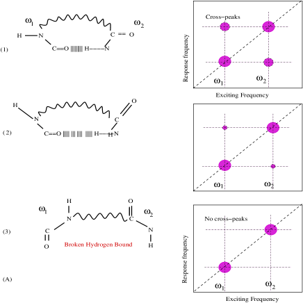
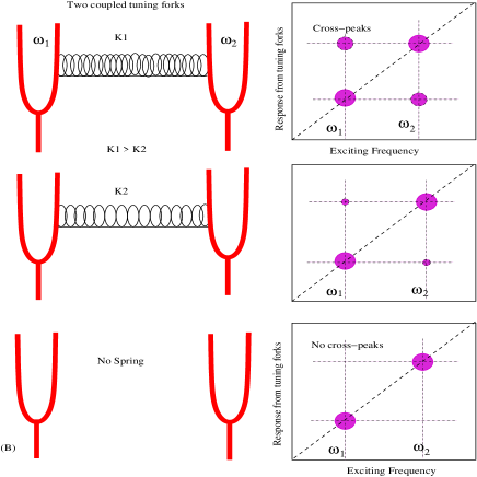
Figure 12: (A) 2D spectroscopy can track (in real time) the changes in the molecular structure. In the above example hydrogen bound breaking dynamics between two chemical groups is shown. Two chemical groups have characteristic frequencies $\omega_{1}$ and $\omega_{2}$. Two peaks appear at these frequencies in the 2D photon echo spectrum. Two cross-peaks also appear as shown which is due to the coupling of these two chemical groups. The coupling is due to the hydrogen bound. When the bound is broken this cross-peaks also disappear. (B) A mechanical analogy: The occurrence of cross peaks in the exciting-response frequency spectrum is due to the spring coupling between two tuning forks of frequency $\omega_{1}$ and $\omega_{2}$. The amplitude of cross-peaks in the 2D spectrum measures the strength of coupling. When the spring constant decreases the cross peaks diminishes and finally goes to zero with no coupling.

2D photon echo spectroscopy can also tell us about the real time resonance coupling dynamics and bond breaking dynamics (Fig. 12). Consider that we have two tuning forks with characteristic frequencies $\omega_{1}$ and $\omega_{2}$. Let us excite this system with a spectrum of frequencies and detect the amplitude of vibration with some frequency analyzer (some electronic instrument) and plot various frequencies along the x-axis (exciting frequencies) and y-axis (detecting frequencies). We will see two peaks occurring at $\omega_{1}$ and $\omega_{2}$ in the ”2D spectrum” (along the diagonal Fig. 12).

Now consider that our tuning forks are coupled by some spring (say we have weak coupling). Then again repeat the experiment and plot the 2D spectrum. This time we will see, along with the diagonal peaks, two ”cross-peaks” along the anti-diagonal direction. These cross peaks are the consequence of coupling. If we further reduce the spring coupling the magnitude of these cross peaks diminish and finally disappear with our removal of coupling springs.

This mechanical analogy can be directly applied to the changes in the molecular structure. In Fig. 1 hydrogen bound breaking dynamics between two chemical groups is shown. Two chemical groups have characteristic frequencies $\omega_{1}$ and $\omega_{2}$. Two peaks appear at these frequencies in the 2D photon echo spectrum. Two cross-peaks also appear as shown which is due to the coupling of these two chemical groups. The coupling is due to the hydrogen bound. When the bound is broken this cross-peaks also disappear. This can be tracked in real time by varying the magnitude of the population time. Similarly in the electronic spectrum the cross peaks tell us about the electronic coupling between the chromophores (the system-system coupling, usually denoted as $J$ or $V$) also called resonance coupling. The oscillation in the magnitude of the cross peaks show the oscillations of the pigments about their equilibrium positions (in physical space) as the variation about the equilibrium position modulate the resonance coupling strength.

A brief mathematical formulation can be described as follows. In semi-classical approximation for field-matter interaction the interaction Hamiltonian is written as

$$H_{int}=-{\bf\mu}.{\bf E}({\bf r},t)$$ (33)

Here dipole approximation (weak variation of the electric field amplitude over the size of the pigment) is used. If the magnitude of the above Hamiltonian is much weaker than the magnitude of the pigment Hamiltonian $H_{pig}=H_{e}+H_{ph}+H_{e-ph}$, then the $H_{int}$ can be treated as a perturbation.

The dynamics of the total system (the pigment) can be described by Liouville-von Neumann equation for the density matrix $\rho$.

$$\frac{\partial\rho}{\partial t}=-\frac{i}{\hbar}[H_{pig}+H_{int},\rho]$$ (34)

Now consider that the sample is interrogated with three consecutive (in time) ultra short laser pulses. Treating $H_{int}$ as a perturbation the third order density matrix is given as

$$\rho^{(3)}({\bf r},t)=(\frac{i}{\hbar})^{3}\int_{0}^{\infty}dt_{3}\int_{0}^{\infty}dt_{2}\int_{0}^{\infty}dt_{1}\Theta(t_{3})e^{-\frac{i}{\hbar}\mathcal{L}t_{3}}\times$$ (35)

$$L_{\mu}\Theta(t_{2})e^{-\frac{i}{\hbar}\mathcal{L}t_{2}}L_{\mu}\Theta(t_{1})e^{-\frac{i}{\hbar}\mathcal{L}t_{1}}L_{\mu}\rho(-\infty){\bf E}({\bf r},t-t_{3}){\bf E}({\bf r},t-t_{3}-t_{2}){\bf E}({\bf r},t-t_{3}-t_{2}-t_{1}).$$

Here $\mathcal{L}*=[H_{pig},*]$ and $L_{\mu}*=[{\bf\mu},*]$. Experimentally we do not measure $\rho(t)$ but the induced polarization $P^{(3)}({\bf r},t)=tr[\mu\rho^{(3)}(t)]$.

$${\bf P}^{(3)}({\bf r},t)=(\frac{i}{\hbar})^{3}\int_{0}^{\infty}dt_{3}\int_{0}^{\infty}dt_{2}\int_{0}^{\infty}dt_{1}R^{(3)}(t_{3},t_{2},t_{1}){\bf E}({\bf r},t-t_{3}){\bf E}({\bf r},t-t_{3}-t_{2}){\bf E}({\bf r},t-t_{3}-t_{2}-t_{1}).$$ (36)

The 3rd order response function is given as

$$R^{(3)}(t_{3},t_{2},t_{1})=(\frac{i}{\hbar})^{3}\Theta(t_{3})\Theta(t_{2})\Theta(t_{1})\left\langle[[[\mu(t_{3}+t_{2}+t_{1}),\mu(t_{2}+t_{1})],\mu(t_{1})],\mu(0)\rho(0)]\right\rangle.$$ (37)

The time dependence of $\mu$ can be shifted to the time dependence of the density matrix using time evolution operators (resulting $\mu$ as time independent). Ultimately one have to take the trace over the bath modes thus one will end up having an expression involving time depended reduced density matrix elements of the system.

The electric field of the incoming pulses can be given as

$${\bf E}({\bf r},t)=\sum_{i=1}^{3}\left({\bf n_{i}}E_{i}(t)e^{(i.{\bf k_{i}.r}-i\omega_{i}t)}+c.c.\right)$$ (38)

Where ${\bf n}$ is the unit vector pointing in the direction of the field and $E(t)$ is the temporal envelope of the pulse. The non-linear polarization can also be expanded in the Fourier components

$${\bf P}^{(3)}({\bf r},t)=\sum_{l}{\bf P}^{(3)}_{l}(t)e^{i{\bf k_{l}.r}-i\omega_{l}t}$$ (39)

Where

$${\bf k}_{l}=\pm{\bf k}_{1}\pm{\bf k}_{2}\pm{\bf k}_{3},~{}~{}~{}~{}\omega_{l}=\pm\omega_{1}\pm\omega_{2}\pm\omega_{3}$$ (40)

This non-linear polarization will emit a signal electric field in the phase matching direction. It can be shownLABEL:( if the electric field amplitude varies slowly over the pigment size and if the refractive index of the material is frequency independent) that

$${\bf E}_{signal}^{(3)}\propto{\bf P}^{(3)}$$ (41)

Now under the impulsive limit (excitation femtosecond laser pulses as delta functions) $E_{1}(t)=E_{1}\delta(t+T+\tau),~{}~{}E_{2}(t)=E_{2}\delta(t+T),~{}~{}E_{3}(t)=E_{3}\delta(t)$ the signal electric field becomes proportional to the response function. The Double Fourier transform of the signal field gives the complex 2D spectrum

$$\tilde{E}_{signal}^{(3)}(\omega_{t},T,\omega_{\tau})\propto\int_{-\infty}^{+\infty}dt\int_{-\infty}^{+\infty}d\tau R^{(3)}(t,T,\tau)e^{i\omega_{t}t}e^{i\omega_{\tau}\tau}$$ (42)

This is the 2D photon echo signal. The whole problem boils down to the calculation of 3rd order response function which further involves the time evolution of the reduced density matrix.

References

- (1) An Inconvenient Truth, a 2006 documentary film, directed by Davis Guggenheim.
- (2) H. Van Amerongen, L. Valkunas, and R. Van Grondelle, Photosynthesis Excitons (World Scientific, Singapore, 2000); R. E. Blankenship, Molecular Mechanisms of Photosysnthesis (World Scientific, London, 2002).
- (3) T. Förster, Ann. Phys. 437, 55(1948); A. G. Redfield, IBM J Res Dev, 1, 19 (1957).
- (4) G. S. Engel, T. R. Calhoun, E. L. Read, T. K. Ahn, T. Mancal, Y.-C. Cheng, R. E. Blankenship, and G. R. Fleming, Nature 446, 782(2007); H. Lee, Y. C. Cheng, G. R. Fleming, Science 316, 1462 (2007); E. Collini, G. D. Scholes, Science 323, 369 (2009).
- (5) E.Collini, C.Y. Wong, K.E. Wilk, P.M.G. Curmi, P. Brumer and G.D. Scholes, Nature 463, 644 (2010); K. Panitchayangkoon, D. Hayesa, K. A. Fransteda, J. R. Carama, E. Harela, J. Wenb, R. E. Blankenshipb, and Gregory S. Engel, PNAS, 107, 12767 (2010); E. Harel and G. S. Engel, PNAS (accepted) 2012; D. Hayes and G.S. Engel, Phil. Tran. Royal Soc. A, (accepted) 2011; J. R. Caram and G. S. Engel, Far. Dis., 153(1) 93-104 (2011); D. Hayes and G. S. Engel, Far. Dis. 150(1) 459-469 (2011); G. S. Engel, Chem. Procedia. 3(1) 222-231 (2011); D. Hayes, G. S. Engel, Biophys.Jour., 100:8 2043-2052 (2011); D. Hayes, G. Panitchayangkoon, K.A. Fransted, J. R. Caram, J. Wen, K. F. Freed, G. S. Engel, New J. Phys. 12: 065042 (2010); E. L. Read, G. S. Schlau-Cohen, G. S. Engel, J. Wen, R. E. Blankenship, G. R. Fleming, Biophys. Jour., 95, 847-856 (2008); Y.-C. Cheng, G. S. Engel, G. R. Fleming, Chem. Phys. 341, 285-295 (2007); A. B. Doust, K. E. Wilk, P. M. G. Curmi, and G. D. Scholes, J. Photochem. Photobiol. A Chem. 184, 1–17 (2006); G. R. Fleming, G. D. Scholes, Yuan-Chung Cheng, “Quantum Effects in Biology”, Procedia Chemistry (in press), Proceedings of the 22nd Solvay Conference on Chemistry.
- (6) V. May and O. Kuhn, Charge and Energy Transfer Dynamics in Molecular Systems, 3rd edition, (Wiley-VCH, Weinheim, 2011); H.-P. Breuer and F. Petruccione, The Theory of Open Quantum Systems, (Oxford University Press, New York, 2002) (Wiley-VCH, New York, 2004); U. Weiss, Quantum Dissipative Systems, 3rd Ed. (World Scientific, Singapore, 2008).
- (7) M. Yang and G. R. Fleming, Chem. Phys. 275, 355 (2002).
- (8) Navinder Singh and Paul Brumer, Faraday Disc. 153, 41 (2011); Navinder Singh and Paul Brumer, Mol. Phys. (2012), to appear.
- (9) A. Ishizaki and G. R. Fleming, J. Chem. Phys.130, 234111 (2009); A. Ishizaki and G. R. Fleming, PNAS, 106, 17255 (2009).
- (10) P. Linz, Analytical and Numerical Methods for Volterra Equations, SIAM, Philadelphia (1985), ISBN: 0-89871-198-3.
- (11) A. Ishizaki and G. R. Fleming, PNAS, 106, 17255 (2009).
- (12) Y. Tanimura and R. Kubo, J. Phys. Soc. Jpn., 58, 101 (1989).
- (13) S. Rackovsky and R. Silbey, Mol. Phys., bf 25, 61 (1973); B. Jackson and R. Silbey, J. Chem Phys., 78, 4193 (1983); R. Silbey and R. A. Harris, J. Chem. Phys., 80, 2615 (1984); R. Silbey, Annu. Rev. Phys. Chem. 27, 203 (1976).
- (14) S. Jang, Y. -C. Cheng, D. R. Reichman, and J. D. Eaves, J. Chem. Phys. 129, 101104 (2008); Seogjoo Jang, J. Chem. Phys. 131, 164101 (2009).
- (15) Navinder Singh, submitted to Phys. Rev. E. (2011).
- (16) A. A. Ovchinnikov and N. S. Erikhman, Sov. Phys. JETP, 40, 733 (1974).
- (17) E. A. Novikov, Zh. Eksp. Teor. Fiz., 47, 1919 (1964) [Sov. Phys. JETP, 20. 1990 (1965)].
- (18) R. Kubo, in: Fluctuation relaxation and resonance in magnetic systems, Scottish Universities’ Summer School, 1961, edited by D. Ter Haar (Oliver and Boyd, London).
- (19) Minhaeng Cho, Chem. Rev., 108, 1331 (2008); M. Khalil, N. Demirdoven, and A. Tomakoff, J. Phys. Chem. A, 107, 5258 (2003); S. Mukamel, Annu. Rev. Phys. Chem., 51, 691 (2000); D. M. Jonas, Annu. Rev. Phys. Chem., 54, 425 (2003); S. Mukamel, Principles of Nonlinear Optical Spectroscopy (Oxford University Press, New York, 1995).
- (20) G. S. Engel, T. R. Calhoun, E. L. Read, T. K. Ahn, T. Mancal, Y.-C. Cheng, R. E. Blankenship, and G. R. Fleming, Nature 446, 782(2007).
- (21) First, why bath should re-organize? The answer is: when an electronic transition happens it disturbes the charge distribution in the molecule (pigment). Nuclear co-ordinates re-organize in real space to reach a new equilibrium configuration.
- (22) The phenomenon of motional(exchange) narrowing is important in the elongation of cross peaks in 2D photon echo spectra (private communication with Prof. Gregory Scholes). A simple reason how motional narrowing can cause long coherence is that narrowing of the absorption band (shrinking of the absorption band) means reduction in the “frictional drag” on the excitation, hence the decreasing decoherence rate [see also, second last paragraph of the first column on page 769 of G. D. Scholes, G. R. Fleming, Alexandra Olaya-Castro, and Rienk van Grondelle, Nat. Chem., 3, 763 (2011)].