Covariance approximation for large multivariate spatial data sets with an application to multiple climate model errors

Abstract

This paper investigates the cross-correlations across multiple climate model errors. We build a Bayesian hierarchical model that accounts for the spatial dependence of individual models as well as cross-covariances across different climate models. Our method allows for a nonseparable and nonstationary cross-covariance structure. We also present a covariance approximation approach to facilitate the computation in the modeling and analysis of very large multivariate spatial data sets. The covariance approximation consists of two parts: a reduced-rank part to capture the large-scale spatial dependence, and a sparse covariance matrix to correct the small-scale dependence error induced by the reduced rank approximation. We pay special attention to the case that the second part of the approximation has a block-diagonal structure. Simulation results of model fitting and prediction show substantial improvement of the proposed approximation over the predictive process approximation and the independent blocks analysis. We then apply our computational approach to the joint statistical modeling of multiple climate model errors.

, and T1This publication is based in part on work supported by Award No. KUS-C1-016-04, made by King Abdullah University of Science and Technology (KAUST). t2Supported in part by NSF Grant DMS-10-07618. t3Supported in part by NSF Grant DMS-09-06532. t4Supported in part by NSF Grant DMS-09-07170 and the NCI Grant CA57030.

1 Introduction

This paper addresses the problem of combining multiple climate model outputs while accounting for dependence across different models as well as spatial dependence within each individual model. To study the impact of human activity on climate change, the Intergovernmental Panel on Climate Change (IPCC) is coordinating efforts worldwide to develop coupled atmosphere-ocean general circulation models (AOGCMs). Various organizations around the world are developing state-of-the-art numerical models and currently 20$+$ climate models are available. A growing body of literature also exists that studies multiple climate model outputs [e.g., Tebaldi et al. (2005); Furrer et al. (2007); Jun, Knutti and Nychka (2008a, 2008b); Smith et al. (2009); Sain and Furrer (2010); Christensen and Sain (2010); Sain, Furrer and Cressie (2011)]. One important research problem of interest regarding these climate model outputs is to investigate the cross-correlations across climate model errors [Tebaldi and Knutti (2007); Jun, Knutti and Nychka (2008a, 2008b); Knutti et al. (2010b)]. Climate models are constantly copied and compared, and successful approximation schemes are frequently borrowed from other climate models. Therefore, many of the climate models are dependent to some degree and thus may be expected to have correlated errors. For similar reasons, we may expect correlations to be higher between the models developed by the same organization. Indeed, Jun, Knutti and Nychka (2008a, 2008b) quantified cross-correlations between pairs of climate model errors at each spatial location and the results show that many climate model errors have high correlations and some of the models developed by the same organizations have even higher correlated errors. Note that throughout the paper, we use the terminology “error” rather than “bias” to describe the discrepancy between the climate model output and the true climate. The reason is that we consider the “error” as a stochastic process rather than a deterministic quantity.

In this paper we build a joint statistical model for multiple climate model errors that accounts for the spatial dependence of individual models as well as cross-covariance across different climate models. Our model offers a nonseparable cross-covariance structure. We work with a climate variable, surface temperature, from multiple global AOGCM outputs. We include several covariates such as latitude, land/ocean effect, and altitude in the mean structure. The marginal and cross-covariance structure of climate model errors are modeled using a spatially varying linear model of co-regionalization (LMC). The resulting covariance structure is nonstationary and is able to characterize the spatially varying cross-correlations between multiple climate model errors. Our modeling approach complements in many ways the previous work of Jun, Knutti and Nychka (2008b). Jun, Knutti and Nychka (2008b) used kernel smoothing of the products of climate model errors to obtain cross-correlations and did not formally build joint statistical models for multiple climate model outputs. One direct product of our model is a continuous surface map for the cross-covariances. Our Bayesian hierarchical modeling approach also provides uncertainty measures of the estimations of the spatially varying cross-covariances, while it is a challenging task to achieve for the kernel smoothing approach. In Jun, Knutti and Nychka (2008b) they fit each climate model error separately to a univariate regression model before obtaining the kernel estimate of cross-correlations. They only considered land/ocean effect in the covariance structure. In our approach, we not only include the land/ocean effect but also altitude and latitude in the cross-covariance structure of the climate model errors. As a statistical methodology, joint modeling is more efficient in estimating model parameters. Moreover, our approach is able to produce spatial prediction or interpolation and thus is potentially useful as a statistical downscaling technique for multivariate climate model outputs.

The naive implementation of our modeling approach faces a big computational challenge because it requires repeated calculations of quadratic forms in large inverse covariance matrices and determinants of large covariance matrices, needed in the posterior distribution and likelihood evaluation. This is a well-known challenge when dealing with large spatial data sets. Various methods have been proposed in the literature to overcome this challenge, including likelihood approximation [Vecchia (1988); Stein, Chi and Welty (2004); Fuentes (2007); Caragea and Smith (2007)], covariance tapering [Furrer, Genton and Nychka (2006); Kaufman, Schervish and Nychka (2008)], Gaussian Markov random-field approximation [Rue and Tjelmeland (2002); Rue and Held (2005)] and reduced rank approximation [Higdon (2002); Wikle and Cressie (1999); Ver Hoef, Cressie and Barry (2004); Kammann and Wand (2003); Cressie and Johannesson (2008); Banerjee et al. (2008)]. Most of these methods focus on univariate processes. One of the exceptions is the predictive process approach [Banerjee et al. (2008)]. Although the predictive process approach is applicable to our multivariate model, it is not a perfect choice because it usually fails to accurately capture local, small-scale dependence structures [Finley et al. (2009)].

We develop a new covariance approximation for multivariate processes that improves the predictive process approach. Our covariance approximation, called the full-scale approximation, consists of two parts: The first part is the same as the multivariate predictive process, which is effective in capturing large-scale spatial dependence; and the second part is a sparse covariance matrix that can approximate well the small-scale spatial dependence, that is, unexplained by the first part. The complementary form of our covariance approximation enables the use of reduced-rank and sparse matrix operations and hence greatly facilitates computation in the application of the Gaussian process models for large data sets. Although our method is developed to study multiple climate model errors, it is generally applicable to a wide range of multivariate Gaussian process models involving large spatial data sets. The full-scale approximation has been previously studied for univariate processes in Sang and Huang (2010), where covariance tapering was used to generate the second part of the full-scale approximation. In addition to the covariance tapering, this paper considers using block diagonal covariance for the same purpose. Simulation results of model fitting and prediction using the full-scale approximation show substantial improvement over the predictive process and the independent blocks analysis. We also find that using the block diagonal covariance achieves even faster computation than using covariance tapering with comparable performance.

Our work contributes to the literature of statistical modeling of climate model outputs. Despite high correlations between the errors of some climate models, it has been commonly assumed that climate model outputs and/or their errors are independent of each other [Giorgi and Mearns (2002); Tebaldi et al. (2005); Green, Goddard and Lall (2006); Furrer et al. (2007); Smith et al. (2009); Furrer and Sain (2009); Tebaldi and Sansó (2009)]. Only recently, several authors have attempted to build joint models for multiple climate model outputs that account for the dependence across different climate models. For example, Sain and Furrer (2010) used a multivariate Markov random-field (MRF) approach to analyze 20-year average precipitation data from five different regional climate model (RCM) outputs. They presented a method to combine the five RCM outputs as a weighted average and the weights are determined by the cross-covariance structure of different RCM outputs. Sain, Furrer and Cressie (2011) built multivariate MRF models for the analysis of two climate variables, precipitation and temperature, from six ensemble members of an RCM (three ensemble members for each climate variable). Their model is designed for what they call simple ensembles that resulted from the perturbed initial conditions of one RCM, not for multiple RCMs. Unlike our approach, the MRF models are best suited for lattice data, and it might be difficult for their approach to incorporate covariates information into the cross-covariance structure. Christensen and Sain (2010) used the factor model approach to integrate multiple RCM outputs. Their analysis is done at each spatial location independently and, thus, the spatial dependence across grid pixels is not considered in the analysis. We believe our modeling and computational method provides a flexible alternative to these existing approaches in joint modeling of climate model outputs.

The remainder of the paper is organized as follows. In Section 2 we detail the motivating data set of climate model errors and present a multivariate spatial process model to analyze the data. Section 3 introduces a covariance approximation method to address the model fitting issues with large multivariate spatial data sets. In Section 4 we present a simulation study to explore properties of the proposed computational method. The full analysis of the climate errors data is then offered in Section 5. Finally, we conclude the paper in Section 6.

2 Data and the multivariate spatial model

2.1 Data

Our goal is to build a joint statistical model for multiple climate model errors. By climate model error, we mean the difference between the climate model output and the corresponding observations. We use surface temperature (unit: K) with global coverage obtained from the AOGCM simulations as well as the observations. The observations are provided by the Climate Research Unit (CRU), East Anglia, and the Hadley Centre, UK MetOffice [Jones et al. (1999); Rayner et al. (2006)]. The data (both climate model outputs and observations) are monthly averages given on a regular spatial grid (the resolution is $5^{\circ}\times 5^{\circ}$). A list of the climate models used in this study is given in Table 1. These climate models are developed by different modeling groups worldwide, under the coordination of the IPCC, and they use common initial conditions. Each model has their own grid resolution. We consider the 30 year interval 1970–1999 and due to the lack of observations near the polar area, we only consider temperature data taken between latitude $45^{\circ}$ S and $72^{\circ}$ N, with the full longitude ranging from $180^{\circ}$ W to $180^{\circ}$ E. We still have missing observations at a few pixels and we impute by taking the average of the spatially neighboring cells (all eight neighboring cells if all are available). We study climatological mean state in the sense that we first get a seasonal average temperature (e.g., an average of the monthly temperature from December to February) and then average it over 30 years. We denote this 30 year average of Boreal winter temperature by DJF.

Table 1: The names of modeling groups, country, IPCC I.D. and resolutions of the IPCC model outputs used in the study. The resolution of the observations is $5^{\circ}\times 5^{\circ}$

				Resolution
	Group	Country	IPCC I.D.	(longitude${}\bolds{\times}{}$latitude)
1	US Dept. of Commerce/NOAA/	USA	GFDL-CM2.0	$2.5^{\circ}\times 2^{\circ}$.
	Geophysical Fluid
	Dynamics Laboratory
2	US Dept. of Commerce/NOAA/	USA	GFDL-CM2.1	$2.5^{\circ}\times 2^{\circ}$.
	Geophysical Fluid
	Dynamics Laboratory
3	Hadley Centre for Climate	UK	UKMO-HadCM3	0$3.79^{\circ}\times 2.47^{\circ}$
	Prediction and Research/
	Met Office
4	Hadley Centre for Climate	UK	UKMO-HadGEM1	$1.875^{\circ}\times 1.24^{\circ}$
	Prediction and Research/
	Met Office
5	LASG/Institute of	China	FGOALS-g1.0	$2.81^{\circ}\times 3^{\circ}$0.
	Atmospheric Physics

As mentioned earlier, we calculate model errors by taking the difference between climate model outputs and actual observations. However, as shown in Table 1, the climate model outputs and the observations are at different spatial grid resolutions. Since the observations have the coarsest grid, we use the bilinear interpolation of the model output to the observational grid. That is, at each grid pixel (in the observation grid), we use the weighted average of model outputs at the four nearest pixels in the model output grid. Figure 2 displays pictures of the climate model errors for the five climate models listed in Table 1. First note that the errors of model 5 are significantly larger in the higher latitudes and in the Himalayan area compared to the errors of the other models. The climate model error maps exhibit quite similar patterns among the models developed by the same group, although the errors for model 1 in the mid-latitude area of the Northern Hemisphere appear to be larger in magnitude compared to those of model 2. All the models have larger errors in the Northern Hemisphere and the errors are large over the high altitude area and high latitude area.

We focus on climate model errors in this paper. Since the climate model error is defined as the difference between a climate model’s output and the corresponding observations (we use the observation minus the model output), we are effectively building a joint model for multiple climate model outputs with the observations as their means (although we have to be careful about the sign of the fixed mean part). It would be tantalizing to build an elaborate joint statistical model of multiple climate model outputs as well as the observations directly at their original spatial grid resolutions. This direct modeling approach would require a statistical representation of the true climate and of the climate model outputs, both of which are challenging tasks. It would be hard to model the true climate in a reasonably complex way and the characteristics of observation errors and model errors may not be simple. Therefore, we do not pursue this direction in this paper.

2.2 Multivariate spatial regression models

Let $\mathbf{Y}(\mathbf{s})=(Y_{1}(\mathbf{s}),\ldots,\break Y_{R}(\mathbf{s}))^{T}$ be an $R\times 1$ response vector along with a $p\times R$ matrix of regressors $\mathbf{X}(\mathbf{s})=(\mathbf{X}_{1}(\mathbf{s}),\ldots,\mathbf{X}_{R}(\mathbf{s}))$ observed at location $\mathbf{s}\in D$, where $D$ is the region of interest. For our application, $Y_{i}(\mathbf{s})$ represents the error of climate model $i$ at location $\mathbf{s}$ for $i=1,\ldots,5$, $\mathbf{X}_{i}(\mathbf{s})$ the corresponding covariates, and $D$ represents the surface of the globe. We consider the multivariate spatial regression model

$$\mathbf{Y}(\mathbf{s})=\mathbf{X}^{T}(\mathbf{s})\bolds{\beta}+\mathbf{w}(\mathbf{s})+\bolds{\varepsilon}(\mathbf{s}),\qquad\mathbf{s}\in D\subseteq\mathbb{R}^{d},$$ (1)

where $\bolds{\beta}=(\beta_{1},\ldots,\beta_{p})^{T}$ is a $p\times 1$ column vector of regression coefficients, $\mathbf{w}(\mathbf{s})$ is a multivariate spatial process whose detailed specification is given below, and the process $\bolds{\varepsilon}(\mathbf{s})=(\varepsilon_{1}(\mathbf{s}),\ldots,\varepsilon_{R}(\mathbf{s}))^{T}$ models the measurement error for the responses. The measurement error process is typically assumed to be spatially independent, and at each location, $\bolds{\varepsilon}(\mathbf{s})\sim\operatorname{MVN}(\mathbf{0},\bolds{\Sigma}_{\bolds{\varepsilon}})$, where MVN stands for the multivariate normal distribution, and $\bolds{\Sigma}_{\bolds{\varepsilon}}$ is an $R\times R$ covariance matrix.

As a crucial part of model (1), the spatial process $\mathbf{w}(\mathbf{s})=(w_{1}(\mathbf{s}),\ldots,\break w_{R}(\mathbf{s}))^{T}$ captures dependence both within measurements at a given site and across the sites. We model $\mathbf{w}(\mathbf{s})$ as an $R$-dimensional zero-mean multivariate Gaussian process: $\mathbf{w}(\mathbf{s})\sim\operatorname{MVN}(\mathbf{0},\Gamma_{\mathbf{w}}(\cdot,\cdot))$, where the cross-covariance matrix function of $\mathbf{w}(\mathbf{s})$ is defined as $\Gamma_{\mathbf{w}}(\mathbf{s},\mathbf{s}^{\prime})=[\operatorname{Cov}(w_{r}(\mathbf{s}),w_{r^{\prime}}(\mathbf{s}^{\prime}))]_{r,r^{\prime}=1}^{R}$. For any integer $n$ and any collection of sites $\mathcal{S}=(\mathbf{s}_{1},\ldots,\mathbf{s}_{n})$, we denote the multivariate realizations of $\mathbf{w}(\mathbf{s})$ at $\mathcal{S}$ as an $nR\times 1$ vector $\mathbf{w}=(\mathbf{w}^{T}(\mathbf{s}_{1}),\ldots,\break\mathbf{w}^{T}(\mathbf{s}_{n}))^{T}$, which follows an $nR\times 1$ multivariate normal distribution $\mathbf{w}\sim\operatorname{MVN}(\mathbf{0},\bolds{\Sigma}_{\mathbf{w}})$, where $\bolds{\Sigma}_{\mathbf{w}}=[\Gamma_{\mathbf{w}}(\mathbf{s}_{i},\mathbf{s}_{j})]_{i,j=1}^{n}$ is an $nR\times nR$ matrix that can be partitioned as an $n\times n$ block matrix with the $(i,j)$th block being the $R\times R$ cross-covariance matrix $\Gamma_{\mathbf{w}}(\mathbf{s}_{i},\mathbf{s}_{j})$. In the multivariate setting, we require a valid cross-covariance function such that the resultant $nR\times nR$ covariance matrix, $\bolds{\Sigma}_{\mathbf{w}}$, is positive definite.

There have been many works on the construction of flexible cross-covariance functions [Mardia and Goodall (1993); Higdon, Swall and Kern (1999); Gaspari and Cohn (1999); Higdon (2002); Ver Hoef, Cressie and Barry (2004); Gelfand et al. (2004); Majumdar and Gelfand (2007); Gneiting, Kleiber and Schlather (2010); Jun (2009); Apanasovich and Genton (2010)]. The model in Mardia and Goodall (1993) assumes separable cross-covariance functions. Higdon (2002) employs discrete approximation to the kernel convolution based on a set of prespecified square-integrable kernel functions. The model in Gneiting, Kleiber and Schlather (2010) is isotropic and the covariance model requires the same spatial range parameters when there are more than two processes. The model of Apanasovich and Genton (2010) is developed to model stationary processes and its extension to nonstationary processes is not obvious.

We adopt the LMC approach [Wackernagel (2003); Gelfand et al. (2004)] which has recently gained popularity in multivariate spatial modeling due to its richness in structure and feasibility in computation. Suppose that $\mathbf{U}(\mathbf{s})=[U_{q}(\mathbf{s})]_{q=1:Q}$ is a $Q\times 1$ process with each $U_{q}(\mathbf{s})$ independently modeled as a univariate spatial process with mean zero, unit variance and correlation function $\rho_{q}(\cdot,\cdot)$. The cross-covariance function of $\mathbf{U}(\mathbf{s})$ is a diagonal matrix that can be written as $\Gamma_{\mathbf{u}}(\mathbf{s},\mathbf{s}^{\prime})=\bigoplus_{q=1}^{Q}\rho_{q}(\mathbf{s},\mathbf{s}^{\prime})$, where $\bigoplus$ is the direct sum matrix operator [e.g., Harville (2008)]. The LMC approach assumes that $\mathbf{w}(\mathbf{s})=\mathbf{A}(\mathbf{s})\mathbf{U}(\mathbf{s})$, where $\mathbf{A}(\mathbf{s})$ is an $R\times Q$ transformation matrix, that is, nonsingular for all $\mathbf{s}$. For identifiability purposes and without loss of generality, $\mathbf{A}(\mathbf{s})$ can be taken to be a lower-triangular matrix. It follows that the constructed cross-covariance function for $\mathbf{w}(\mathbf{s})$ under this model is $\Gamma_{\mathbf{w}}(\mathbf{s},\mathbf{s}^{\prime})=\mathbf{A}(\mathbf{s})\Gamma_{\mathbf{u}}(\mathbf{s},\mathbf{s}^{\prime})\mathbf{A}^{T}(\mathbf{s}^{\prime})$. An alternative expression for the cross-covariance function is $\Gamma_{\mathbf{w}}(\mathbf{s},\mathbf{s}^{\prime})=\sum_{q=1}^{Q}\mathbf{a}_{q}(\mathbf{s})\mathbf{a}_{q}^{T}(\mathbf{s}^{\prime})\rho_{q}(\mathbf{s},\mathbf{s}^{\prime})$, where $\mathbf{a}_{q}(\mathbf{s})$ is the $q$th column vector of $\mathbf{A}(\mathbf{s})$. The cross-covariance matrix for the realizations $\mathbf{w}$ at $n$ locations $\mathcal{S}$ can be written as a block partitioned matrix $\bolds{\Sigma}_{\mathbf{w}}$ with $n\times n$ blocks, whose $(i,j)$th block is $\mathbf{A}(\mathbf{s}_{i})\Gamma_{\mathbf{u}}(\mathbf{s}_{i},\mathbf{s}_{j})\mathbf{A}^{T}(\mathbf{s}_{j})$. We can express $\bolds{\Sigma}_{\mathbf{w}}$ as

$$\bolds{\Sigma}_{\mathbf{w}}=\Biggl{[}\bigoplus_{i=1}^{n}\mathbf{A}(\mathbf{s}_{i})\Biggr{]}\Biggl{[}\bigoplus_{q=1}^{Q}\rho_{q}(\mathbf{s}_{i},\mathbf{s}_{j})\Biggr{]}_{i,j=1}^{n}\Biggl{[}\bigoplus_{i=1}^{n}\mathbf{A}^{T}(\mathbf{s}_{i})\Biggr{]}=\mathcal{A}\bolds{\Sigma}_{\mathbf{u}}\mathcal{A}^{T},$$ (2)

where $\mathcal{A}$ is a block-diagonal matrix with $n\times n$ blocks whose $i$th diagonal block is $\mathbf{A}(\mathbf{s}_{i})$, $\bigoplus_{q=1}^{Q}\rho_{q}(\mathbf{s}_{i},\mathbf{s}_{j})$ is a $Q\times Q$ diagonal matrix with $\rho_{q}(\mathbf{s}_{i},\mathbf{s}_{j})$’s as its diagonals, and $\bolds{\Sigma}_{\mathbf{u}}$ is an $(n\times n)$-block partitioned matrix with $\Gamma_{\mathbf{u}}(\mathbf{s}_{i},\mathbf{s}_{j})$ as its $(i,j)$th block.

For our climate model application, we utilize the multivariate model (1). Here, we have $R=5$ since five climate model errors are considered. In the LMC model, the number of latent processes, $Q$, can take a value from $1$ to $R$. When $Q<R$, the multivariate process is represented in a lower dimensional space and dimensionality reduction is achieved. In this paper, our goal is to obtain a rich, constructive class of multivariate spatial process models and, therefore, we assume a full rank LMC model with $Q=R=5$. We do not include the spatial nugget effect $\bolds{\varepsilon}$ in the model. For the regression mean, $\mathbf{X}^{T}(\mathbf{s})\bolds{\beta}$, we use $p=8$ covariates: Legendre polynomials [Abramowitz and Stegun (1964)] in latitude of order $0$ to $4$ with sine of latitude as their arguments, an indicator of land/ocean (we give 1 if the domain is over the land and 0 otherwise), longitude (unit: degree), and the altitude (altitude is set to be zero over the ocean). We scale the altitude variable (unit: m) by dividing it by 1000 to make its range comparable to other covariates. Our covariates specification is similar to Sain, Furrer and Cressie (2011) except that we use multiple terms for latitude effects in order to have enough flexibility to capture the dependence of the process on the entire globe.

For each location $\mathbf{s}$, we model $\mathbf{A}(\mathbf{s})$ as a $5\times 5$ lower triangular matrix. Two model specifications for $\mathbf{A}(\mathbf{s})$ are considered. In one specification, we assume the linear transformation to be independent of space, that is, $\mathbf{A}(\mathbf{s})=\mathbf{A}$. Thus, we have $\mathbf{A}(\mathbf{s})=[a_{ij}]_{i,j=1:5}$ with $a_{ij}$ being nonzero constants for $1\leq i\leq j\leq 5$ and $a_{ij}=0$ for $i>j$. To avoid an identifiability problem, we let $a_{ii}>0$ for $i=1,\ldots,5$. If the $U_{q}(\mathbf{s})$ are stationary, this specification results in a stationary cross-covariance structure. In particular, if the $U_{q}(\mathbf{s})$ are identically distributed, this specification results in a separable cross-covariance structure similarly to Sain and Furrer (2010). In the second specification, we assume that $\mathbf{A}(\mathbf{s})$ vary over space. Specifically, the $(i,j)$th entry of $\mathbf{A}(\mathbf{s})$, $a_{ij}(\mathbf{s})$, is modeled as $a_{ij}(\mathbf{s})=\mathbf{X}_{A}^{T}(\mathbf{s})\bolds{\eta}_{ij}$ for $1\leq i\leq j\leq 5$, where $\mathbf{X}_{A}(\mathbf{s})$ is a $5\times 1$ covariate vector at location $\mathbf{s}$ and consists of Legendre polynomials in latitude of order $0$ to $2$, an indicator of land/ocean, and the scaled altitude. The dimension of $\bolds{\eta}_{ij}$ is $5\times 1$. This specification induces nonstationary and nonseparable cross-covariance structure. Note that, similar to the first specification, to avoid an identifiability problem, we let $a_{ii}(\mathbf{s})=|\mathbf{X}_{A}^{T}(\mathbf{s})\bolds{\eta}_{ii}|$ for $i=1,\ldots,5$. Gelfand et al. (2004) proposed to model each element of $\mathbf{A}(\mathbf{s})$ as a spatial process, but in practice such an approach is usually computationally too demanding to be used for large scale problems. Moreover, there might be identifiability problems if we do not constrain some of the elements in $\mathbf{A}(\mathbf{s})$. Thus, we do not consider this option in our paper. For the correlation function of each latent process $U_{q}(\mathbf{s})$, we consider a Matérn correlation function on a sphere, where the chordal distance is used. For any two locations on the globe $(L_{i},l_{i}),i=1,2$, where $L_{i}$ and $l_{i}$ denote latitude and longitude, respectively, the chordal distance is defined as

$$\operatorname{ch}((L_{1},l_{1}),(L_{2},l_{2}))$$

$$\qquad=2R_{\mathrm{earth}}\biggl{\{}\sin^{2}\biggl{(}\frac{L_{1}-L_{2}}{2}\biggr{)}+\cos L_{1}\cos L_{2}\sin^{2}\biggl{(}\frac{l_{1}-l_{2}}{2}\biggr{)}\biggr{\}}^{1/2}.$$

Here $R_{\mathrm{earth}}$ is the radius of the Earth. Jun, Knutti and Nychka (2008b) showed that the maximum likelihood estimates of the smoothness parameters for all of the climate models in Table 1 (except for model 4) are close to 0.5. Therefore, we fix the smoothness parameter values for all the processes in $\mathbf{U}$ to be 0.5 and this is the same as using an exponential correlation function for each $U_{q}(\mathbf{s})$.

3 Model implementation and covariance approximation

3.1 Model fitting

We adopt a Bayesian approach that specifies prior distributions on the parameters. Posterior inference for the model parameters is implemented by model fitting with Gibbs samplers [Gelfand and Smith (1990)] and Metropolis–Hastings updating [Gelman et al. (2004)]. We set $\bolds{\beta}$ to have a $p$-dimensional multivariate normal distribution prior with large variances. The prior assignment for the covariance parameters for each $\mathbf{U}_{i}$ depends upon the specific choice of the correlation functions. In general, the spatial range parameters are weakly identifiable, and, hence, reasonably informative priors are needed for satisfactory MCMC behavior. We set prior distributions for the spatial range parameters relative to the size of their domains, for instance, by setting the prior means to reflect one’s prior belief about the practical spatial range of the data. For the LMC setting with a constant $\mathbf{A}$, we may assign truncated normal priors with positive value support or inverse gamma priors with infinite variances for the diagonal entries, and normal priors for other entries. For the spatially varying LMC setting, the priors for the coefficients $\bolds{\eta}_{ij}$ are normal distributions with large variances.

Given $n$ locations in the set $\mathcal{S}=\{\mathbf{s}_{1},\ldots,\mathbf{s}_{n}\}$, the realization of the response vector at these locations can be collectively denoted as $\mathbb{Y}=(\mathbf{Y}(\mathbf{s}_{1})^{T},\break\ldots,\mathbf{Y}(\mathbf{s}_{n})^{T})^{T}$, and the corresponding matrix of covariates is $\mathbb{X}=(\mathbf{X}(\mathbf{s}_{1}),\ldots,\break\mathbf{X}(\mathbf{s}_{n}))^{T}$. The data likelihood can be obtained easily from the fact that $\mathbb{Y}\sim\operatorname{MVN}(\mathbb{X}\bolds{\beta},\bolds{\Sigma}_{\mathbf{w}}+\mathbf{I}_{n}\otimes\bolds{\Sigma}_{\bolds{\varepsilon}})$, where $\bolds{\Sigma}_{\mathbf{w}}$ is given by (2). Generically denoting the set of all model parameters by $\Omega$, the MCMC method is used to draw samples of the model parameters from the posterior: $p(\Omega|\mathbb{Y})\propto P(\Omega)P(\mathbb{Y}|\Omega)$. Assuming the prior distribution of $\bolds{\beta}$ is $\operatorname{MVN}(\bolds{\mu}_{\bolds{\beta}},\bolds{\Sigma}_{\bolds{\beta}})$, the posterior samples of $\bolds{\beta}$ are updated from its full conditional $\operatorname{MVN}(\bolds{\mu}_{\bolds{\beta}|\cdot},\bolds{\Sigma}_{\bolds{\beta}|\cdot})$, where $\bolds{\Sigma}_{\bolds{\beta}|\cdot}=[\bolds{\Sigma}_{\bolds{\beta}}^{-1}+\mathbb{X}^{T}(\bolds{\Sigma}_{\mathbf{w}}+\mathbf{I}_{n}\otimes\bolds{\Sigma}_{\bolds{\varepsilon}})^{-1}\mathbb{X}]^{-1}$, and $\bolds{\mu}_{\bolds{\beta}|\cdot}=\bolds{\Sigma}_{\bolds{\beta}|\cdot}\mathbb{X}^{T}(\bolds{\Sigma}_{\mathbf{w}}+\mathbf{I}_{n}\otimes\bolds{\Sigma}_{\bolds{\varepsilon}})^{-1}\mathbb{Y}$. All the remaining parameters have to be updated using Metropolis–Hastings steps.

Spatial interpolation in the multivariate case allows one to better estimate one variable at an unobserved location by borrowing information from co-located variables. It is also called “cokriging” in geostatistics. The multivariate spatial regression model provides a natural way to do cokriging. For example, under the Bayesian inference framework, the predictive distribution for $\mathbf{Y}(\mathbf{s}_{0})=[Y_{i}(\mathbf{s}_{0})]_{i=1:p}$ at a new location $\mathbf{s}_{0}$ is a Gaussian distribution with

$$\mathrm{E}[\mathbf{Y}(\mathbf{s}_{0})|\Omega,\mathbb{Y}]=\mathbf{X}^{T}(\mathbf{s}_{0})\bolds{\beta}+\mathbf{h}(\mathbf{s}_{0})(\bolds{\Sigma}_{\mathbf{w}}+\mathbf{I}_{n}\otimes\bolds{\Sigma}_{\bolds{\varepsilon}})^{-1}(\mathbb{Y}-\mathbb{X}\bolds{\beta})$$

and

$$\operatorname{Cov}[\mathbf{Y}(\mathbf{s}_{0})|\Omega,\mathbb{Y}]=\Gamma_{\mathbf{w}}(\mathbf{s}_{0},\mathbf{s}_{0})+\bolds{\Sigma}_{\bolds{\varepsilon}}-\mathbf{h}(\mathbf{s}_{0})(\bolds{\Sigma}_{\mathbf{w}}+\mathbf{I}_{n}\otimes\bolds{\Sigma}_{\bolds{\varepsilon}})^{-1}\mathbf{h}^{T}(\mathbf{s}_{0}),$$

where $\mathbf{h}(\mathbf{s}_{0})=[\Gamma_{\mathbf{w}}(\mathbf{s}_{0},\mathbf{s}_{i})]_{i=1:n}$ is the $R\times nR$ cross-covariance matrix between $\mathbf{w}(\mathbf{s}_{0})$ and $\{\mathbf{w}(\mathbf{s}_{i}),i=1,\ldots,n\}$.

The computationally demanding part in the model fitting is to calculate the quadratic form of the inverse of the $nR\times nR$ matrix $\bolds{\Sigma}_{\mathbf{w}}+\mathbf{I}_{n}\otimes\bolds{\Sigma}_{\bolds{\varepsilon}}$, whose computational complexity is of the order $O((nR)^{3})$. This computational issue is often referred to as “the big n problem.” In our climate model application, we have 1,656 locations for each of the five climate models, that is, $n=1\mbox{,}656$ and $R=5$. Although the inversion of the matrix can be facilitated by the Cholesky decomposition and linear solvers, computation remains expensive when $nR$ is big, especially for the spatially varying LMC models which involve a relatively large number of parameters and hence require multiple likelihood evaluations at each MCMC iteration. We introduce covariance approximation below as a way to gain computational speedup for the implementation of the LMC models.

3.2 Predictive process approximation

In this subsection we review the multivariate predictive process approach by Banerjee et al. (2008) and point out its drawbacks to motivate our new covariance approximation method. The predictive process models consider a fixed set of “knots” $\mathcal{S}^{\ast}=\{\mathbf{s}^{\ast}_{1},\ldots,\break\mathbf{s}^{\ast}_{m}\}$ that are chosen from the study region. The Gaussian process $\mathbf{w}(\mathbf{s})$ in model (1) yields an $mR$ random vector $\mathbf{w}^{\ast}=[\mathbf{w}(\mathbf{s}_{i}^{\ast})]_{i=1}^{m}$ over $\mathcal{S}^{\ast}$. The Best Linear Unbiased Predictor (BLUP) of $\mathbf{w}(\mathbf{s})$ at any fixed site $\mathbf{s}$ based on $\mathbf{w}^{\ast}$ is given by $\tilde{\mathbf{w}}(\mathbf{s})=E\{\mathbf{w}(\mathbf{s})|\mathbf{w}^{\ast}\}$. Being a conditional expectation, it immediately follows that $\tilde{\mathbf{w}}(\mathbf{s})$ is an optimal predictor of $\mathbf{w}(\mathbf{s})$ in the sense that it minimizes the mean squared prediction error $E\{\|\mathbf{w}(\mathbf{s})-\mathbf{f}(\mathbf{w}^{*})\|^{2}\}$ over all square-integrable (vector-valued) functions $\mathbf{f}(\mathbf{w}^{*})$ for Gaussian processes, and over all linear functions without the Gaussian assumption. Banerjee et al. (2008) refer to $\tilde{\mathbf{w}}(\mathbf{s})$ as the predictive process derived from the parent process $\mathbf{w}(\mathbf{s})$.

Since the parent process $\mathbf{w}(\mathbf{s})$ is an $R$-dimensional zero-mean multivariate Gaussian process with the cross-covariance function $\Gamma_{\mathbf{w}}(\mathbf{s},\mathbf{s}^{\prime})=\operatorname{Cov}(\mathbf{w}(\mathbf{s}),\break\mathbf{w}(\mathbf{s}^{\prime}))$, the multivariate predictive process has a closed-form expression

$$\tilde{\mathbf{w}}(\mathbf{s})=\operatorname{Cov}(\mathbf{w}(\mathbf{s}),\mathbf{w}^{\ast})\operatorname{Var}^{-1}(\mathbf{w}^{\ast})\mathbf{w}^{\ast}=\mathcal{C}_{\mathbf{w}}(\mathbf{s},\mathcal{S}^{\ast};\bolds{\theta})\mathcal{C}_{\mathbf{w}}^{\ast-1}(\bolds{\theta})\mathbf{w}^{\ast},$$ (3)

where $\mathcal{C}_{\mathbf{w}}(\mathbf{s},\mathcal{S}^{\ast};\bolds{\theta})=[\Gamma_{\mathbf{w}}(\mathbf{s},\mathbf{s}^{\ast}_{1};\bolds{\theta}),\ldots,\Gamma_{\mathbf{w}}(\mathbf{s},\mathbf{s}^{\ast}_{m};\bolds{\theta})]$ is an $R\times mR$ cross-covariance matrix between $\mathbf{w}(\mathbf{s})$ and $\{\mathbf{w}(\mathbf{s}^{*}),\mathbf{s}^{*}\in\mathcal{S}^{\ast}\}$, and $\mathcal{C}_{\mathbf{w}}^{\ast}(\bolds{\theta})=[\Gamma_{\mathbf{w}}(\mathbf{s}^{\ast}_{i},\mathbf{s}^{\ast}_{j};\break\bolds{\theta})]_{i,j=1}^{m}$ is the $mR\times mR$ cross-covariance matrix of $\mathbf{w}^{\ast}=[\mathbf{w}(\mathbf{s}^{\ast}_{i})]_{i=1}^{m}$ [see, e.g., Banerjee, Carlin and Gelfand (2004)].

The multivariate predictive process $\tilde{\mathbf{w}}(\mathbf{s})$ is still a zero mean Gaussian process, but now with a fixed rank cross-covariance function given by $\Gamma_{\tilde{\mathbf{w}}}(\mathbf{s},\mathbf{s}^{\prime})=\mathcal{C}_{\mathbf{w}}(\mathbf{s},\mathcal{S}^{\ast};\bolds{\theta})\mathcal{C}_{\mathbf{w}}^{\ast-1}(\bolds{\theta})\mathcal{C}_{\mathbf{w}}^{T}(\mathbf{s}^{\prime},\mathcal{S}^{\ast};\bolds{\theta})$. Let $\tilde{\mathbf{w}}=[\tilde{w}(\mathbf{s}_{i})]_{i=1}^{n}$ be the realization of $\tilde{\mathbf{w}}(\mathbf{s})$ at the set $\mathcal{S}$ of the observed locations. It follows that $\tilde{\mathbf{w}}\sim\operatorname{MVN}(\mathbf{0},\bolds{\Sigma}_{\tilde{\mathbf{w}}})$, where $\bolds{\Sigma}_{\tilde{\mathbf{w}}}=\mathcal{C}_{\mathbf{w}}(\mathcal{S},\mathcal{S}^{\ast};\bolds{\theta})\mathcal{C}_{\mathbf{w}}^{\ast-1}(\bolds{\theta})\mathcal{C}_{\mathbf{w}}^{T}(\mathcal{S},\mathcal{S}^{\ast};\bolds{\theta})$, and $\mathcal{C}_{\mathbf{w}}(\mathcal{S},\mathcal{S}^{\ast};\bolds{\theta})$ is an $nR\times mR$ matrix that can be partitioned as an $n\times 1$ block matrix whose $i$th block is given by $\mathcal{C}_{\mathbf{w}}(\mathbf{s}_{i},\mathcal{S}^{\ast};\bolds{\theta})$.

Replacing $\mathbf{w}(\mathbf{s})$ in (1) with the fixed rank approximation $\tilde{\mathbf{w}}(\mathbf{s})$, we obtain the following multivariate regression model:

$$\mathbf{Y}(\mathbf{s})=\mathbf{X}^{T}(\mathbf{s})\bolds{\beta}+\tilde{\mathbf{w}}(\mathbf{s})+\bolds{\varepsilon}(\mathbf{s}),$$ (4)

which is called the predictive process approximation of model (1). Based on this approximation, the data likelihood can be obtained using $\mathbb{Y}\sim\operatorname{MVN}(\mathbb{X}\bolds{\beta},\break\mathcal{C}_{\mathbf{w}}(\mathcal{S},\mathcal{S}^{\ast};\bolds{\theta})\mathcal{C}_{\mathbf{w}}^{\ast-1}(\bolds{\theta})\mathcal{C}_{\mathbf{w}}^{T}(\mathcal{S},\mathcal{S}^{\ast};\bolds{\theta}))+\mathbf{I}_{n}\otimes\bolds{\Sigma}_{\bolds{\varepsilon}})$. When the number of knots $m$ is chosen to be substantially smaller than $n$, computational gains are achieved since the likelihood evaluation that initially involves inversion of $nR\times nR$ matrices can be done by inverting much smaller $mR\times mR$ matrices.

The multivariate predictive process is an attractive reduced rank approach to deal with large spatial data sets. It encompasses a very flexible class of spatial cross-covariance models since any given multivariate spatial Gaussian process with a valid cross-covariance function would induce a multivariate predictive process. Since the predictive process is still a valid Gaussian process, the inference and prediction schemes for multivariate Gaussian spatial process models that we described in Section 3.1 can be easily implemented here.

However, the predictive process models share one common problem with many other reduced rank approaches: They generally fail to capture local/small scale dependence accurately [Stein (2008); Finley et al. (2009); Banerjee et al. (2010)] and thus lead to biased parameter estimations and errors in prediction.

To see the problems with the multivariate spatial process $w(\mathbf{s})$ in (1), we consider the following decomposition of the parent process:

$$\mathbf{w}(\mathbf{s})=\tilde{\mathbf{w}}(\mathbf{s})+\bigl{(}\mathbf{w}(\mathbf{s})-\tilde{\mathbf{w}}(\mathbf{s})\bigr{)}.$$ (5)

We call $\mathbf{w}(\mathbf{s})-\tilde{\mathbf{w}}(\mathbf{s})$ the residual process. The decomposition in (5) immediately implies a decomposition of the covariance function of the process $\mathbf{w}(\mathbf{s})$:

$$\Gamma_{\mathbf{w}}(\mathbf{s},\mathbf{s}^{\prime})=\Gamma_{\tilde{\mathbf{w}}}(\mathbf{s},\mathbf{s}^{\prime})+\bigl{(}\Gamma_{\mathbf{w}}(\mathbf{s},\mathbf{s}^{\prime})-\Gamma_{\tilde{\mathbf{w}}}(\mathbf{s},\mathbf{s}^{\prime})\bigr{)},$$ (6)

where $\Gamma_{\mathbf{w}}(\mathbf{s},\mathbf{s}^{\prime})-\Gamma_{\tilde{\mathbf{w}}}(\mathbf{s},\mathbf{s}^{\prime})$ is the cross-covariance function of the residual process $\mathbf{w}(\mathbf{s})-\tilde{\mathbf{w}}(\mathbf{s})$. Note that for any arbitrary set of $n$ locations $\mathcal{S}$, $\bolds{\Sigma}_{\mathbf{w}}-\bolds{\Sigma}_{\tilde{\mathbf{w}}}=[\Gamma_{\mathbf{w}}(\mathbf{s}_{i},\mathbf{s}_{j})]_{i,j=1}^{n}-[\Gamma_{\tilde{\mathbf{w}}}(\mathbf{s}_{i},\mathbf{s}_{j})]_{i,j=1}^{n}$ is the conditional variance–covariance matrix of $\mathbf{w}$ given $\mathbf{w}^{\ast}$, and hence a nonnegative definite matrix. Using the multivariate predictive process to approximate $\mathbf{w}(\mathbf{s})$, we discard the residual process $\bolds{\Sigma}_{\mathbf{w}}-\bolds{\Sigma}_{\tilde{\mathbf{w}}}$ entirely and thus fail to capture the dependence it carries. This is indeed the fundamental issue that leads to biased estimation in the model parameters.

To understand and illustrate the issue with the predictive process due to ignoring the residual process, we consider a univariate stationary Gaussian process and we remark that the multivariate predictive process shares the same problems. Assume the covariance function of the parent process is $\mathbf{C}_{w}(\mathbf{s},\mathbf{s}^{\prime})=\sigma^{2}\rho_{w}(\mathbf{s},\mathbf{s}^{\prime})$, where $\rho_{w}(\mathbf{s},\mathbf{s}^{\prime})$ is the correlation function and $\sigma^{2}$ is the variance, that is, constant over space. Assume $\tau^{2}$ is the nugget variance. The variance of the corresponding predictive process at location $\mathbf{s}$ is given by $\sigma_{\tilde{w}}^{2}(\mathbf{s})=\sigma^{2}\rho_{w}^{T}(\mathbf{s},\mathcal{S}^{\ast})\rho_{w}^{-1}(\mathcal{S}^{\ast},\mathcal{S}^{\ast})\rho_{w}(\mathbf{s},\mathcal{S}^{\ast})$, where $\rho_{w}(\mathbf{s},\mathcal{S}^{\ast})$ is the correlation vector between $w(\mathbf{s})$ and $\{w(\mathbf{s}^{*}),\mathbf{s}^{*}\in\mathcal{S}^{\ast}\}$, and $\rho_{w}(\mathcal{S}^{\ast},\mathcal{S}^{\ast})$ is the correlation matrix of the realizations of $w(\mathbf{s})$ at the knots in the set $\mathcal{S}^{\ast}$. From the nonnegative definiteness of the residual covariance function, we obtain the inequality $\sigma^{2}_{w}(\mathbf{s})\geq\sigma_{\tilde{w}}^{2}(\mathbf{s})$. Equality holds when $\mathbf{s}$ belongs to $\mathcal{S}^{*}$. Therefore, the predictive process produces a lower spatial variability. Banerjee et al. (2010) proved that there are systematic upward biases in likelihood-based estimates of the spatial variance parameter $\sigma^{2}$ and the nugget variance $\tau^{2}$ using the predictive process model as compared to the parent model. Indeed, the simulation results in Finley et al. (2009) and Banerjee et al. (2010) showed that both $\sigma^{2}$ and $\tau^{2}$ are significantly overestimated especially when the number of knots is small. Our simulation study to be presented in Section 4 also shows that predictive processes produce biased estimations of model parameters in the multivariate spatial case.

3.3 Full-scale covariance approximation

Motivated by the fact that discarding the residual process $\tilde{\bolds{\varepsilon}}(\mathbf{s})=\mathbf{w}(\mathbf{s})-\tilde{\mathbf{w}}(\mathbf{s})$ is the main cause of the problem associated with the multivariate predictive process, we seek to complement the multivariate predictive process by adding a component that approximates the residual cross-covariance function while still maintaining computational efficiency. We approximate the residual cross-covariance function by

$$\Gamma_{\tilde{\bolds{\varepsilon}}}(\mathbf{s},\mathbf{s}^{\prime})=[\Gamma_{\mathbf{w}}(\mathbf{s},\mathbf{s}^{\prime};\bolds{\theta})-\Gamma_{\tilde{\mathbf{w}}}(\mathbf{s},\mathbf{s}^{\prime};\bolds{\theta})]\circ\mathcal{K}(\mathbf{s},\mathbf{s}^{\prime}),$$ (7)

where $\circ$ denotes the Schur product (or entrywise product) of matrices, and the matrix-valued function $\mathcal{K}(\mathbf{s},\mathbf{s}^{\prime})$, referred to as the modulating function, has the property of being a zero matrix for a large proportion of possible spatial location pairs $(\mathbf{s},\mathbf{s}^{\prime})$. The zeroing property of the modulating function implies that the resulting cross-covariance matrix is sparse and, thus, sparse matrix algorithms are readily applicable for fast computation. We will introduce below modulating functions that have zero value when $\mathbf{s}$ and $\mathbf{s}^{\prime}$ are spatially farther apart. For such choices of the modulating function, the effect of multiplying a modulating function in (7) is expected to be small, since the residual process mainly captures the small scale spatial variability.

Combining (6) with (7), we obtain the following approximation of the cross-covariance function:

$$\Gamma_{\mathbf{w}}^{\dagger}(\mathbf{s},\mathbf{s}^{\prime})=\Gamma_{\tilde{\mathbf{w}}}(\mathbf{s},\mathbf{s}^{\prime})+\Gamma_{\tilde{\bolds{\varepsilon}}}(\mathbf{s},\mathbf{s}^{\prime}).$$ (8)

Note that the first part of the cross-covariance approximation, $\Gamma_{\tilde{\mathbf{w}}}$, is the result of the predictive process approximation and should capture well the large scale spatial dependence, while the second part, $\Gamma_{\tilde{\bolds{\varepsilon}}}$, should capture well the small scale spatial dependence. We refer to (8) as the full-scale approximation (FSA) of the original cross-covariance function.

Using the FSA, the covariance matrix of the data $\mathbb{Y}$ from model (1) is approximated by

$$\bolds{\Sigma}_{\mathbb{Y}}=\bolds{\Sigma}_{\tilde{\mathbf{w}}}+\bolds{\Sigma}_{\tilde{\bolds{\varepsilon}}}+\mathbf{I}_{n}\otimes\bolds{\Sigma}_{\bolds{\varepsilon}},$$ (9)

where $\bolds{\Sigma}_{\tilde{\mathbf{w}}}=\mathcal{C}_{\mathbf{w}}(\mathcal{S},\mathcal{S}^{\ast};\bolds{\theta})\mathcal{C}_{\mathbf{w}}^{\ast-1}(\bolds{\theta})\mathcal{C}_{\mathbf{w}}^{T}(\mathcal{S},\mathcal{S}^{\ast};\bolds{\theta})$, and $\bolds{\Sigma}_{\tilde{\bolds{\varepsilon}}}=[\Gamma_{\tilde{\bolds{\varepsilon}}}(\mathbf{s}_{i},\mathbf{s}_{j};\bolds{\theta})]_{i,j=1}^{n}$. The structure of the covariance matrix (9) allows efficient computation of the quadratic form of its inverse and its determinant. Using the Sherman–Woodbury–Morrison formula, we see that the inverse of $\bolds{\Sigma}_{\mathbb{Y}}$ can be computed by

$$(\bolds{\Sigma}_{\tilde{\mathbf{w}}}\,{+}\,\bolds{\Sigma}_{\tilde{\bolds{\varepsilon}}}\,{+}\,\mathbf{I}_{n}\otimes\bolds{\Sigma}_{\bolds{\varepsilon}})^{-1} \,{=}\, (\bolds{\Sigma}_{\tilde{\bolds{\varepsilon}}}\,{+}\,\mathbf{I}_{n}\,{\otimes}\,\bolds{\Sigma}_{\bolds{\varepsilon}})^{-1}\,{-}\,(\bolds{\Sigma}_{\tilde{\bolds{\varepsilon}}}\,{+}\,\mathbf{I}_{n}\,{\otimes}\,\bolds{\Sigma}_{\bolds{\varepsilon}})^{-1}\mathcal{C}_{\mathbf{w}}(\mathcal{S},\mathcal{S}^{\ast})$$

$$\!{}{\times}\,\{\mathcal{C}_{\mathbf{w}}^{\ast}\,{+}\,\mathcal{C}_{\mathbf{w}}(\mathcal{S},\mathcal{S}^{\ast})^{T}(\bolds{\Sigma}_{\tilde{\bolds{\varepsilon}}}\,{+}\,\mathbf{I}_{n}\,{\otimes}\,\bolds{\Sigma}_{\bolds{\varepsilon}})^{-1}\mathcal{C}_{\mathbf{w}}(\mathcal{S},\mathcal{S}^{\ast})\}^{-1}$$

$$\!{}{\times}\,\mathcal{C}_{\mathbf{w}}(\mathcal{S},\mathcal{S}^{\ast})^{T}(\bolds{\Sigma}_{\tilde{\bolds{\varepsilon}}}\,{+}\,\mathbf{I}_{n}\,{\otimes}\,\bolds{\Sigma}_{\bolds{\varepsilon}})^{-1}.$$

The determinant is computed as

$$\operatorname{det}(\bolds{\Sigma}_{\tilde{\mathbf{w}}}+\bolds{\Sigma}_{\tilde{\bolds{\varepsilon}}}+\mathbf{I}_{n}\otimes\bolds{\Sigma}_{\bolds{\varepsilon}})$$

$$\qquad=\operatorname{det}\{\mathcal{C}_{\mathbf{w}}^{\ast}+\mathcal{C}_{\mathbf{w}}(\mathcal{S},\mathcal{S}^{\ast})^{T}(\bolds{\Sigma}_{\tilde{\bolds{\varepsilon}}}+\mathbf{I}_{n}\otimes\bolds{\Sigma}_{\bolds{\varepsilon}})^{-1}\mathcal{C}_{\mathbf{w}}(\mathcal{S},\mathcal{S}^{\ast})\}$$ (11)

$$\qquad\quad{}\times\{\operatorname{det}(\mathcal{C}_{\mathbf{w}}^{\ast})\}^{-1}\operatorname{det}(\bolds{\Sigma}_{\tilde{\bolds{\varepsilon}}}+\mathbf{I}_{n}\otimes\bolds{\Sigma}_{\bolds{\varepsilon}}).$$

Notice that $\bolds{\Sigma}_{\tilde{\bolds{\varepsilon}}}+\mathbf{I}_{n}\otimes\bolds{\Sigma}_{\bolds{\varepsilon}}$ is a sparse matrix and $\mathcal{C}_{\mathbf{w}}^{\ast}+\mathcal{C}_{\mathbf{w}}(\mathcal{S},\mathcal{S}^{\ast})^{T}(\bolds{\Sigma}_{\tilde{\bolds{\varepsilon}}}+\mathbf{I}_{n}\otimes\bolds{\Sigma}_{\bolds{\varepsilon}})^{-1}\mathcal{C}_{\mathbf{w}}(\mathcal{S},\mathcal{S}^{\ast})$ is an $mR\times mR$ matrix. By letting $m$ be much smaller than $n$ and letting $\bolds{\Sigma}_{\tilde{\bolds{\varepsilon}}}+\mathbf{I}_{n}\otimes\bolds{\Sigma}_{\bolds{\varepsilon}}$ have a big proportion of zero entries, the matrix inversion and the determinant in (3.3) and (3.3) can be efficiently computed. These computational devices are combined with the techniques described in subsection 3.1 for Bayesian model inference and spatial prediction.

Now we consider one choice of the modulating function, that is, based on a local partition of the domain. Let $B_{1},\ldots,B_{K}$ be $K$ disjoint subregions which divide the spatial domain $D$. The modulating function is taken to be $\mathcal{K}(\mathbf{s},\mathbf{s}^{\prime})=\mathbf{1}_{K\times K}$ if $\mathbf{s}$ and $\mathbf{s}^{\prime}$ belong to the same subregion, and $\mathcal{K}(\mathbf{s},\mathbf{s}^{\prime})=\mathbf{0}_{K\times K}$ otherwise. Voronoi tessellation is one option to construct the disjoint subregions [Green and Sibson (1978)]. This tessellation is defined by a number of centers $\mathbf{c}=(\mathbf{c}_{1},\ldots,\mathbf{c}_{k})$, such that points within $B_{i}$ are closer to $\mathbf{c}_{i}$ than any other center $\mathbf{c}_{j}$, $j\neq i$, that is, $B_{i}=\{\mathbf{s}:\|\mathbf{s}-\mathbf{c}_{i}\|\leq\|\mathbf{s}-\mathbf{c}_{j}\|,j\neq i\}$. Our choice of a Voronoi partitioning scheme is made on the ground of tractability and computational simplicity. We would like to point out that our methodology is not restricted to this choice and any appropriate partitioning strategy for the spatial domain could be adopted. Since the modulating function so specified will generate an approximated covariance matrix with block-diagonal structure, this version of the FSA method is referred to as the FSA-Block.

The FSA-Block method provides an exact error correction for the predictive process within each subregion, that is, $\Gamma_{\mathbf{w}}^{{\dagger}}(\mathbf{s},\mathbf{s}^{\prime})=\Gamma_{\mathbf{w}}(\mathbf{s},\mathbf{s}^{\prime})$ if $\mathbf{s}$ and $\mathbf{s}^{\prime}$ belong to the same subregion, and $\Gamma_{\mathbf{w}}^{\dagger}(\mathbf{s},\mathbf{s}^{\prime})=\Gamma_{\tilde{\mathbf{w}}}(\mathbf{s},\mathbf{s}^{\prime})$ if $\mathbf{s}$ and $\mathbf{s}^{\prime}$ belong to different subregions. Unlike the independent blocks analysis of spatial Gaussian process models, the FSA can take into account large/global scale dependence across different subregions due to the inclusion of the predictive process component. Unlike the predictive process, the FSA can take into account the small scale dependence due to the inclusion of the residual process component. An interesting special case of the FSA-Block is obtained by taking $n$ disjoint subregions, each of which contains only one observation. In this case, $\tilde{\bolds{\varepsilon}}(\mathbf{s})$ is reduced to an independent Gaussian process, that is, $\Gamma_{\tilde{\bolds{\varepsilon}}}(\mathbf{s},\mathbf{s})=\Gamma_{\mathbf{w}}(\mathbf{s},\mathbf{s})-\Gamma_{\tilde{\mathbf{w}}}(\mathbf{s},\mathbf{s})$, and $\Gamma_{\tilde{\bolds{\varepsilon}}}(\mathbf{s},\mathbf{s}^{\prime})=0$ for $\mathbf{s}\neq\mathbf{s}^{\prime}$. In fact, this special case corresponds to the modified predictive process by Finley et al. (2009), that is, introduced to correct the bias for the variance of the predictive process models at each location. Clearly, our FSA-Block is a more general approach since it also corrects the bias for the cross-covariance between two locations that are located in the same subregion.

For the FSA-Block, the computation in (3.3) and (3.3) can be further simplified. Assuming the set of observed locations is grouped by subregions, that is, $\mathcal{S}=\{\mathcal{S}_{B_{1}},\ldots,\mathcal{S}_{B_{K}}\}$, the $nR\times nR$ matrix $\bolds{\Sigma}_{\tilde{\bolds{\varepsilon}}}$ becomes a $K\times K$ block diagonal matrix with the $k$th diagonal block

$$\mathcal{C}_{\mathbf{w}}(\mathcal{S}_{B_{k}},\mathcal{S}_{B_{k}})-\mathcal{C}_{\mathbf{w}}(\mathcal{S}_{B_{k}},\mathcal{S}^{\ast})\mathcal{C}_{\mathbf{w}}^{\ast-1}(\bolds{\theta})\mathcal{C}_{\mathbf{w}}^{T}(\mathcal{S}_{B_{k}},\mathcal{S}^{\ast}),\qquad k=1,\ldots,K,$$

and, thus, $\bolds{\Sigma}_{\tilde{\bolds{\varepsilon}}}+\mathbf{I}_{n}\otimes\bolds{\Sigma}_{\bolds{\varepsilon}}$ is a $K\times K$ block diagonal matrix. The inversion and determinant of this block diagonal matrix can be directly computed efficiently without resorting to general-purpose sparse matrix algorithms if the size of each block is not large.

The computational complexity of the FSA-Block depends on the knot intensity and the block size. If we take equal-sized blocks, then the computational complexity of the log likelihood calculation is of the order $O(nm^{2}R^{3}+nb^{2}R^{3})$, where $m$ is the number of knots and $b$ is the block size. This is much smaller than the original complexity of $O(n^{3}R^{3})$ without using covariance approximation. Moreover, the computational complexity of the FSA can be further reduced using parallel computation by taking advantage of the block diagonal structure of $\bolds{\Sigma}_{\tilde{\bolds{\varepsilon}}}$.

An alternative choice of the modulating function in (7) is to use a positive definite function, that is, identically zero whenever $\|\mathbf{s}-\mathbf{s}^{\prime}\|\geq\gamma$. Such a function is usually called a taper function and $\gamma$ is called the taper range. The resulting FSA method is referred to as the FSA-Taper. In the univariate case, any compactly supported correlation function can serve as a taper function, including the spherical and a family of Wendland functions [see, e.g., Wendland (1995); Wendland (1998); Gneiting (2002)]. Sang and Huang (2010) studied the FSA-Taper and demonstrated its usage for univariate spatial processes. For the multivariate processes considered in this paper, the modulating function $\mathcal{K}(\mathbf{s},\mathbf{s}^{\prime})$ can be chosen as any valid multivariate taper function. One such choice is the matrix direct sum of univariate taper functions, that is, $\mathcal{K}(\mathbf{s},\mathbf{s}^{\prime})={\bigoplus}_{r=1}^{R}K_{r}(\mathbf{s},\mathbf{s}^{\prime};\gamma_{r})$, where $K_{r}$ is a valid univariate taper function with the taper range $\gamma_{r}$ used for the $r$th spatial variable, and different taper ranges can be used for different variables. This cross-independent taper function will work well with the FSA if the cross dependence between co-located variables can be mostly characterized by the reduced rank process $\tilde{\mathbf{w}}$. Using this taper function, the cross-covariance matrix of the residual process, $\bolds{\Sigma}_{\tilde{\bolds{\varepsilon}}}$, can be transformed by row and column permutations to a block-diagonal matrix with $R$ diagonal blocks, whose $r$th diagonal block is an $n\times n$ sparse matrix with the $(i,j)$-entry being $\operatorname{Cov}(\tilde{\varepsilon}_{r}(\mathbf{s}_{i}),\tilde{\varepsilon}_{r}(\mathbf{s}_{j}))=\{\operatorname{Cov}(w_{r}(\mathbf{s}_{i}),w_{r}(\mathbf{s}_{j}))-\operatorname{Cov}(\tilde{w}_{r}(\mathbf{s}_{i}),\tilde{w}_{r}(\mathbf{s}_{j}))\}K_{r}(\mathbf{s}_{i},\mathbf{s}_{j};\gamma_{r})$, where $\tilde{w}_{r}(\mathbf{s})$ is the reduced rank predictive process for the $r$th spatial variable and $\tilde{\varepsilon}_{r}(\mathbf{s})$ is the residual process for the $r$th spatial variable. If we take the same taper range for each spatial variable, the computational complexity of the log likelihood calculation is of the order $O(nm^{2}R^{3}+ng^{2}R)$, where $g$ is the average number of nonzero entries per row in the $n\times n$ residual covariance matrix $[\operatorname{Cov}(\tilde{\varepsilon}_{r}(\mathbf{s}_{i}),\tilde{\varepsilon}_{r}(\mathbf{s}_{j}))]_{i,j=1}^{n}$ for the $r$th spatial variable. This is a substantial reduction from the original computational complexity of $O(n^{3}R^{3})$ without using the covariance approximation.

Use of the FSA involves the selection of knots and the local partitioning or tapering strategy. Given the number of knots, we follow the suggestions by Banerjee et al. (2010) to use the centers obtained from the $K$-means clustering as the knots [e.g., Kaufman and Rousseeuw (1990)]. A careful treatment of the choice of knot intensity $m$ and the number of partitions $K$ or the taper range $\gamma$ will offer good approximation to the original covariance function. Apparently, a denser knot intensity and larger block size or larger taper range will lead to better approximation, at higher computational cost. In principle, we will have to implement the analysis over different choices of $m$ and $K$ or $\gamma$ to weigh the trade-off between inference accuracy and computational cost. We have used the Euclidean distance and taken $m$ to be 225, $K$ to be 36, and $\gamma$ to be 10 for the spherical taper function in our simulation study, and used the chordal distance and taken $m$ to be 200 and $K$ to be 10 in the real application and have found that such choices work well. A full discussion of this issue will be undertaken in future work.

4 Simulation results

In this section we report results from a simulation study to illustrate the performance of the FSA approach and compare it with the predictive process approach and the independent blocks analysis. The computer implementation of all the approaches used in this simulation study and the analysis of multiple climate models in the following section were written in Matlab and run on a processor with dual 2.8 GHz Xeon CPUs and 12 GB memory.

In this simulation study we generated $n=2\mbox{,}000$ spatial locations at random from the square $[0,100]\times[0,100]$. The data generating model is a bivariate LMC model with a constant $2\times 2$ lower triangular transformation matrix $\mathbf{A}$,

$$\mathbf{Y}(\mathbf{s})=\mathbf{A}\mathbf{U}(\mathbf{s})+\bolds{\varepsilon}(\mathbf{s}),$$

where $\bolds{\varepsilon}(\mathbf{s})\sim\operatorname{MVN}(\mathbf{0},\tau^{2}\mathbf{I}_{2})$, and $\mathbf{U}(\mathbf{s})=[U_{q}(\mathbf{s})]_{q=1,2}$ is a $2\times 1$ process with two independent components, each of which is a univariate spatial process with mean zero, unit variance and exponential correlation function. The range parameters for $U_{1}(\mathbf{s})$ and $U_{2}(\mathbf{s})$ are $\phi_{1}=10$ (i.e., such that the spatial correlation is about $0.05$ at 30 distance units) and $\phi_{2}=20$, respectively. The diagonal elements of $\mathbf{A}$ are $a_{11}=1$ and $a_{22}=0.5$, and the nonzero off-diagonal element of $\mathbf{A}$ is $a_{21}=0.5$. We set the nugget variance $\tau^{2}=0.01$.

Given these data, we used the Bayesian MCMC approach to generate samples from the posterior distributions of the model parameters. We assigned $\operatorname{Unif}(1,d_{\mathrm{max}}/3)$ priors to the range parameters $\phi_{1}$ and $\phi_{2}$, where $d_{\mathrm{max}}$ is the maximum distance of all pairs. The diagonal elements of $\mathbf{A}$ and $\tau^{2}$ were assumed to have the inverse gamma distribution with the shape parameter 2 and the scale parameter 1, $\operatorname{IG}(2,1)$, as priors. We assigned a normal prior with large variance for $a_{21}$.

Table 2: The mean and the standard deviations (in parentheses) of the model parameters for the full covariance model, the predictive process approximation, the independent blocks approximation, the FSA-Block and the FSA-Taper

Model	$\bolds{\phi_{1}}$	$\bolds{\phi_{2}}$	$\bolds{a_{11}}$	$\bolds{a_{12}}$	$\bolds{a_{22}}$	$\bolds{\tau^{2}}$
True	100000000.	200000000.	10000000.	0.5000000.	0.5000000.	1.00e–200000000.
Full model	10.47 (1.02)	22.07 (4.69)	0.99 (0.05)	0.51 (0.03)	0.52 (0.05)	1.01e–2 (3.90e–4)
Predictive process	13.32 (2.32)	22.71 (7.35)	1.22 (0.08)	0.66 (0.05)	0.49 (0.06)	0.15 (3.46e–3)000
$m=225$
Independent blocks	04.47 (0.99)	04.94 (1.16)	3.56 (0.39)	1.44 (0.28)	1.96 (0.14)	8.97e–3 (1.18e–3)
$k=36$
FSA-Block	11.36 (2.21)	21.17 (5.24)	1.02 (0.09)	0.53 (0.05)	0.49 (0.05)	1.10e–2 (9.00e–4)
$m=225,k=36$
FSA-Taper	14.89 (1.90)	29.92 (7.41)	1.05 (0.07)	0.58 (0.04)	0.50 (0.05)	8.36e–3 (1.07e–3)
$m=225,\gamma=10$

We compared the model fitting results from four covariance approximation methods: the predictive process, the independent blocks approximation, the FSA-Block and the FSA-Taper. As a benchmark for our comparison, we also fit the original full covariance model without using a covariance approximation. For the predictive process approximation, we used $m=225$ knots. For the independent blocks approximation, we used $K=36$ blocks. For the FSA-Block, we used $m=225$ knots and $K=36$ blocks. For the FSA-Taper, we used $m=225$ and a spherical tapering function with taper range $\gamma=10$. The number of blocks for the FSA-Block and the taper range for the FSA-Taper are selected such that these two FSA methods lead to comparable approximations for the small scale residual covariance. For the above methods, the knots were chosen as the centers from the $K$-means clustering, and the blocks were taken as equal-sized squares that form a partition of the $[0,100]\times[0,100]$ region.

Table 2 displays the Bayesian posterior means and the corresponding posterior standard deviations for the model parameters under each approach. We observe that the diagonal values of $\mathbf{A}$, the range parameter of $U_{1}$, and the nugget variance $\tau^{2}$ are all overestimated by the predictive process. We also notice large biases of the parameter estimates using independent blocks approximation. The FSA-Block provides the most accurate parameter estimation among all the methods.

Table 3: DIC scores and MSPEs for the full covariance model, the predictive process approximation, the independent blocks approximation, the FSA-Block and the FSA-Taper. MSPE-Random is based on a test data set of 200 locations that are randomly selected from $[0,100]\times[0,100]$. MSPE-Hole is based on a test data set of size 200 that consists of 160 randomly selected locations from $[0,100]\times[0,100]$ and 40 random locations within two circles: $\{(x,y);x^{2}+(y-90)^{2}<30\}$ and $\{(x,y);(x-50)^{2}+(y-50)^{2}<35\}$

		Predictive	Independent
		process	blocks	FSA-Block	FSA-Taper
	Full model	$\bolds{m=225}$	$\bolds{K=36}$	$\bolds{m=225}$, $\bolds{K=36}$	$\bolds{m=225}$, $\bolds{\gamma=10}$
DIC	871	2357	3791	918	1547
MSPE-Random	0.12	0.17	0.14	0.12	0.12
MSPE-Hole	0.16	0.26	0.26	0.18	0.18

To gauge the performance on model fitting for different approaches, we used the deviance information criterion [DIC, Spiegelhalter et al. (2002)], which is easily calculated from the posterior samples. From Table 3, we observe that the benchmark full covariance model has the smallest DIC score, indicating the best model fitting. The FSA-Block approach gives a slightly larger DIC score than the full model, while the predictive process and the independent blocks approximation yield significantly larger DIC scores than the FSA and the full model. This result shows that the FSA performs much better than the predictive process and independent blocks approximation in terms of model fitting.

To compare the methods in terms of prediction performance, we computed the mean square prediction errors (MSPE) based on a simulated test data set of 200 locations using the previously simulated data set with observations at 2000 locations as the training set. We experimented with two different kinds of test sets: one set consists of 200 locations randomly selected from $[0,100]\times[0,100]$ and another consists of 160 randomly selected locations from $[0,100]\times[0,100]$ and 40 random locations within two circles: $\{(x,y);x^{2}+(y-90)^{2}<30\}$ and $\{(x,y);(x-50)^{2}+(y-50)^{2}<35\}$. The second interpolation scenario is common in practice where missing data often correspond to sizable gaps/holes.

From Table 2, we see that both the FSA-Block and the FSA-Taper methods lead to much more accurate predictions than the predictive process and the independent blocks approximation. In the scenario of predicting for missing gaps/holes, the advantage of using the FSA approach over the other two approximation approaches is more significant.

To compare the computation efficiency of the covariance approximations for larger data sets, we repeated the simulation study when the number of spatial locations in the training set is increased to 5,000 and the number of locations in the test set to 1,000. We measured the MSPE and the associated computational time based on the prediction at the 1,000 test locations. The test set consists of 800 randomly sampled locations from $[0,100]\times[0,100]$ and 200 locations randomly selected within two circles: $\{(x,y);x^{2}+(y-90)^{2}<30\}$ and $\{(x,y);(x-50)^{2}+(y-50)^{2}<35\}$. The MSPE for each model was obtained by plugging in the true parameter values into the BLUP equation. Pairs of the MSPE and the computational time were obtained by varying the knot intensity for the predictive process model, block size for the independent blocks approximation, knot intensity and block size for the FSA-Block approach, and knot intensity and taper range for the FSA-Taper approach. Figure 1 shows that both the FSA-Taper and the FSA-Block methods outperform the predictive process in terms of their computational efficiency for making predictions. The independent blocks approximation yields much larger MSPE than the other three approaches given the same computational time and we decided not to include its results in Figure 1. It is also noticeable that the required computational time of the FSA-Block approach to obtain the same MSPE is much less than that of the FSA-Taper approach. For this reason, we used the FSA-Block approach to analyze the climate errors data in Section 5.

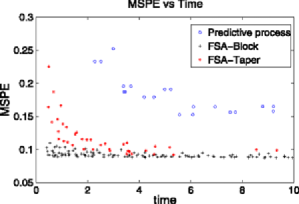
Figure 1: The MSPE versus time plot for the simulation study in Section 4 under the predictive process (circle), the FSA-Block (plus) and the FSA-Taper (star).

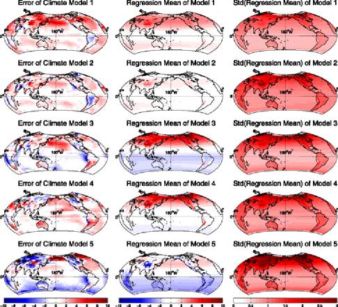
Figure 2: The first column shows the surface maps of climate model errors. The second and the third columns show the estimated mean structure of each climate model error and the associated standard deviations.

We acknowledge that performance for the approximation approaches may depend on the characteristics of spatial data, such as sample size, pattern of sampling locations, spatial smoothness and spatial correlation range. To investigate the effect of spatial correlation range on the performance of the FSA approach, we conducted two other experiments: one with small range parameters $\phi_{1}=5$ and $\phi_{2}=10$, and the other with large range parameters $\phi_{1}=30$ and $\phi_{2}=60$. In the case of small spatial ranges, the independent blocks approximation performed better than the predictive process, while the FSA performed similarly to the independent blocks analysis. In the case of large spatial ranges, the predictive process performed similarly to the FSA and both methods performed significantly better than the independent blocks approximation. These two experiments indicate that both the predictive process and the independent blocks approximation have their modes of successes and failures. Under their failure modes, to achieve accurate model inference and prediction, one has to use either a significantly large rank number $m$ for the predictive process or a very small number of blocks $K$ for the independent blocks approach, therefore, the computational advantages associated with a small $m$ and a large $K$ would disappear. In contrast, by the combining of a small $m$ and a large $K\!$, the FSA-Block flexibly accommodates data sets with either large scale or small scale spatial variations while still maintaining the computational efficiency.

5 Application result

To build a joint model that accounts for the cross-covariance structure of the multiple climate model errors, we fit and compared two versions of the LMC models, corresponding to spatially fixed and spatially varying transformation matrices, as described in Section 2.2. The LMC model specification depends on the ordering of the response variables because of the lower triangular specification of the transformation matrix. When applying the LMC model to the five climate model errors, we tried a few orderings of climate models and found that different orderings may produce different values of parameters but they produced fairly consistent estimates of variances and cross-correlations. Therefore, we chose to present the results based on the order given in Table 1.

We applied the FSA-Block approach to facilitate the computation. We used 225 knots selected by the $K$-means clustering algorithm and divided the study region into 10 regions for subsequent analysis. We assumed the exponential spatial correlation function for each $U_{q}(\mathbf{s})$, and assigned a uniform prior $U(50,4\mbox{,}500)$ for each of the spatial range parameters given that the maximum chordal distance between any two locations is 12,757 km. For each of the coefficients $\bolds{\beta}$ in the regression in model (1), we assumed independent normal priors with mean 0 and variance 1,000. For the LMC model with a constant $\mathbf{A}$, we assumed the diagonal entries to have truncated normal distributions ranging from 0 to $\infty$ and diagonal entries to have normal distributions, with their means being the empirical estimates of $\mathbf{A}$ and variances 1,000. For the spatially varying LMC model with $\mathbf{A}(\mathbf{s})$, we assumed that the intercepts of the coefficients $\bolds{\eta}_{ij}$ in the regression model for $\mathbf{A}(\mathbf{s})$ have normal distributions, with their means being the empirical estimates of $\mathbf{A}$ and variances being 1,000. We set normal priors with mean 0 and variance 1,000 to the other coefficients of $\bolds{\eta}_{ij}$. For each model, we ran 3,000 iterations of MCMC to collect posterior samples after a burn-in period of 1,000 iterations, thinning every third iteration.

The DIC scores of two specifications for $\mathbf{A}$ were compared, one with a constant $\mathbf{A}$ and the other with spatially varying $\mathbf{A}$ depending on polynomials of latitude, land/ocean effect and altitude, as detailed in Section 2.2. The DIC score for the model with a spatially varying $\mathbf{A}(\mathbf{s})$ is 9,901, which is much smaller than the score of 11,975 for the model with a constant $\mathbf{A}$. This suggests that the spatially varying LMC model performs significantly better than the model with a constant $\mathbf{A}$, as we expected. From now on, we present results based solely on the spatially varying LMC model.

Figure 2 shows the estimated mean structure and its standard deviations obtained from the posterior samples. It is interesting to note a clear distinction between model 5 and the rest of the models; for model 5, the estimated means are negative with large magnitudes over high altitude areas, whereas the rest gives large positive values for the estimated mean structure over high latitude areas. This finding is consistent with the result in Jun, Knutti and Nychka (2008b) [note that the model numbers in this paper and the model numbers in Jun, Knutti and Nychka (2008b) are different, although all the models used in this paper are also used in Jun, Knutti and Nychka (2008b)]. Recall that the model error is calculated by subtracting the model output from the observation. The above result suggests that models 1–4 may underestimate the mean state of the surface temperature over the high-altitude and high-latitude regions, and model 5 may overestimate the mean state over the high-altitude area. The estimated mean structure and its associated standard deviations are quite similar for the models developed by the same groups—models 1 and 2 from the GFDL group of NOAA, and models 3 and 4 from the Hadley Centre in the UK. The spatial patterns of the associated standard deviations for those pairs are also quite similar. For all the models, altitude is responsible for the dominant effects in the fixed part of the process and we also see some effects of latitude, although longitude does not seem to be significant in the mean structure. Models 3–5 seem to have large errors in the high-latitude and sea-ice area. The indicator for the land and the ocean is not significant for the mean structure. This may be due to the fact that we already include altitude as a covariate (altitude is positive over the land and zero over the ocean).

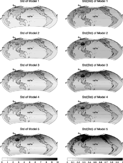
Figure 3: Surface maps of the estimated standard deviations of each climate model (left column) and the associated standard deviations (right column).

Given the posterior samples of the model parameters, we draw samples of the cross-covariance matrix at each location $\mathbf{s}$ based on $\Gamma_{\mathbf{w}}(\mathbf{s},\mathbf{s})=\mathbf{A}(\mathbf{s})\mathbf{A}^{T}(\mathbf{s})$. The diagonals of $\Gamma_{\mathbf{w}}(\mathbf{s},\mathbf{s})$ are the variances of the climate model errors at location $\mathbf{s}$. Figure 3 shows the maps of standard deviations for each model error and the standard deviations of the standard deviations obtained from the posterior samples. The patterns throughout all 5 models are quite consistent; high standard deviations at high altitudes, and standard deviations are higher over the land than over the ocean. For models 1 and 3, latitude seems to be a significant factor. For all the models, given the values of the posterior sample standard deviations of the standard deviations, the spatial patterns that we observe (such as high variances over high altitude or high latitude area) are statistically significant and are not due to random variations in the data. The sea-ice region is one of the places that models in general have trouble. Although we do not have a factor for sea-ice region in the model, we see high standard deviations around sea-ice area. This may be due to the interaction between latitude and the indicator for the land and the ocean. As we expected, model 5 has significantly larger values of standard deviations, especially in high-altitude areas, compared to the rest of the models. The standard deviations of the error of model 5 over the Himalayan area are more than 10. Their associated posterior sample standard deviations are also quite large. Overall, we observe that standard deviations of model errors are slightly higher over the land than over the ocean.

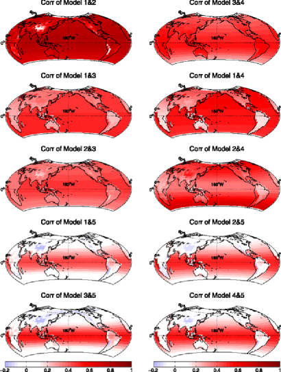
Figure 4: Surface maps of the estimated cross-correlation for each pair of climate model errors.

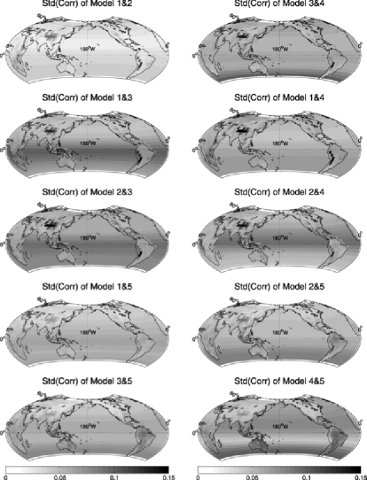
Figure 5: Standard deviation of the estimated cross-correlation for each pair of climate model errors in Figure 4.

Now we discuss the estimates of cross-correlations of different climate model errors. Figure 4 gives the spatial maps of cross-correlations between each pair of climate model errors, obtained from the posterior samples. The corresponding standard deviation of the estimated cross-correlations using the posterior samples are given in Figure 5. In both figures, we use the same color scale across pairs of models to make the comparison easier. First, notice that overall the correlation between models 1 and 2, two models developed by the GFDL group of NOAA, is the highest. For models 1 and 2, overall the correlation values are strikingly high and the associated standard deviation values are close to zero. The maximum correlation value over the entire domain is 0.769, the average of correlations over the ocean is 0.732 with the standard deviation 0.017, and the average over the land is 0.639 with the standard deviation 0.021. Jun, Knutti and Nychka (2008b) also report the highest level of cross-correlation for this pair of models. The cross-correlations between models 3 and 4 (two models developed by the Hadley Centre in the UK) are not as high as those between models 1 and 2 and they are comparable to the cross-correlations between any one of the models 1 and 2 and any one of the models 3 and 4. In addition, the cross-correlation structure between models 1 and 2 shows different spatial patterns compared with that between models 3 and 4. Models 1 and 2 have quite small correlation over high-altitude area, meaning that the two models disagree over high-altitude areas, whereas models 3 and 4 have consistently large correlations over the entire domain. For models 3 and 4, the average of correlations over the land and the ocean are both slightly larger than 0.4. Cross-correlations between model 5 and the rest of the models are quite small in magnitude and the patterns are consistent for all the 4 pairs. Correlations between model 5 and the rest of the models are quite small over the land, over high latitudes in the Northern Hemisphere and over low latitude area in the Southern Hemisphere. From these maps, it is clear that model 5 is significantly different from the rest of the models and this agrees with the result in Jun, Knutti and Nychka (2008b). In many pairs of models, we see clear effects of the indicator for the land and the ocean, and the latitude.

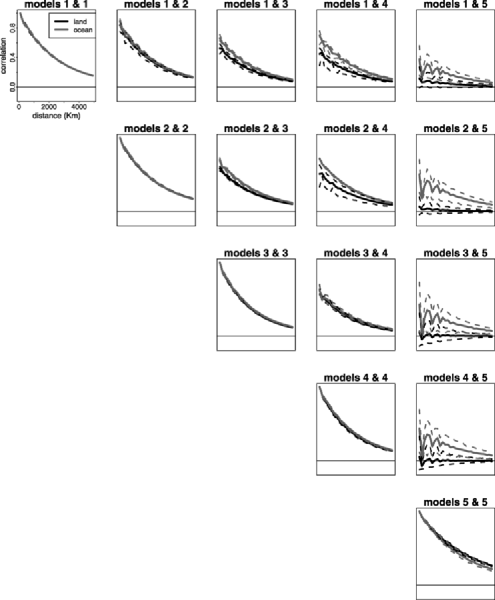
Figure 6: Spatial correlations for pairs of model errors against chordal distance (unit: km). Due to the nonstationarity of the correlation structure, we display the correlation in the following way. For each pair of model errors, we first obtain a $1\mbox{,}656\times 1\mbox{,}656$ cross (or marginal)-correlation matrix given from the posterior mean of the correlations. Then we calculate the averages, the 10th and the 90th percentiles of the correlations within each bin, with 30 equally spaced bins from distance 0 to 5,000 km, separately over the land and the ocean. Solid lines connect the binned averages and dashed lines connect the 10th and the 90th percentiles.

In addition to the cross-correlations at the same location, our method allows us to examine both marginal and cross-covariances/correlations between two different locations, based on the posterior samples. Given that the cross-correlations at the same location are quite different over the land and the ocean, we examined the spatial correlations against spatial distance over the land and the ocean separately. Figure 6 gives both marginal and cross-correlations against chordal distance (unit: km) for pairs of models based on the 1,656 observational grid points. Since we adopted exponential spatial correlation functions for the latent spatial processes $U_{q}(\mathbf{s})$’s in the LMC model with the lower triangular structure for $\mathbf{A}(\mathbf{s})$, the fitted correlation function for model 1 is isotropic. We also note that marginally the model errors 2, 3 and 4 give similar spatial correlation structures over the land and the ocean, while model 5 shows mild discrepancy between the correlations over the land and the ocean. Moreover, the spatial correlation structure of model 5 exhibits a slower spatial decay compared with the rest of the climate model errors. Models developed by the same group (i.e., pairs 1 and 2, and 3 and 4) give similar spatial cross-correlation structure for both over the land and over the ocean. The cross-correlations between model 5 and the rest of the models are close to zero over the land, while those over the ocean are significantly different from zero.

As in Jun, Knutti and Nychka (2008b) and Sain, Furrer and Cressie (2011), we can perform the analysis for the summer season average of Northern Hemisphere (JJA, June–July–August average) in the same way that we did for the DJF averages. We do not include those results for brevity of the paper.

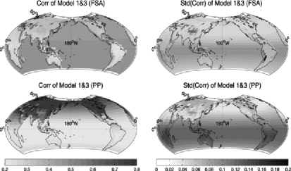
Figure 7: Correlation maps and the associated standard deviation maps between models 1 and 3. The upper panel shows the maps using the FSA-Block approach and the bottom panel shows the maps using the predictive process.

We have also implemented the spatially varying LMC using the predictive process with the same knots as the FSA ($m=200$) for comparison purposes. The DIC score of the predictive process model is 35,526, which is much larger than the DIC score of 9,901 of the FSA model, indicating that the FSA model has a better model fitting for the data. We did not observe significant difference in the estimations for the spatial range parameters. We present in Figure 7 the correlation maps between models 1 and 3 to illustrate the difference between the results of the two approaches. Although, for this real data analysis, the true correlations between models 1 and 3 are unknown, the results obtained from the FSA approach seem to be more reasonable than those from the predictive process. For instance, the map using the FSA approach clearly shows that the correlations over the ocean are in general higher than the correlations over the land, as expected based on previous studies. The map using the predictive process fails to show this pattern. The poor performance of the predictive process in this example might be due to the inadequate number of knots and hence can be remedied by increasing the knots intensity. However, increasing the number of knots will greatly increase the computational time of the predictive process.

6 Discussion

We built a joint spatial model for multivariate climate model errors accounting for their cross-covariances through a spatially varying LMC model. To facilitate Bayesian computation for large spatial data sets, we developed a covariance approximation method for multivariate spatial processes. This full-scale approximation can capture both the large scale and small scale spatial dependence and correct the bias problem of the predictive process.

Our empirical results confirmed that pairs of climate models developed by the same group have high correlations and climate models in general have correlated errors. We also showed that some climate models are very different from other climate models and, thus, the cross-correlations between them are quite small.

In principle, we could combine multiple climate model outputs as a weighted linear combination, along the same lines as Sain and Furrer (2010), based on our modeling approach rather than the Bayesian Gaussian MRF model described in Section 4 of Sain and Furrer (2010). However, recently there have been several papers that raise concerns about the practice of combining multiple climate model outputs through model weighting or ranking [see, e.g., Knutti et al. (2010b); Knutti (2010); Weigel et al. (2010)]. The main concern is the difficulty of interpreting the weighted average of climate models physically. Knutti et al. (2010a) suggest that if model ranking or weighting is applied, both the quality metric and the statistical framework used to construct the ranking or weighting should be recognized. To determine what is the best quality metric in weighting or ranking the climate models is a challenging problem.

We focus on the climate model errors in this paper. It would be interesting to build more elaborate joint models of multiple climate model outputs as well as observations at their original spatial grid resolutions. To follow this path, we need to have a statistical representation of the true climate, which is very challenging. One possibility is to model the observation as the truth, with measurement errors assumed with a simple covariance structure. However, this assumption might not be realistic considering the relatively complex nature of biases and errors in the climate observations.

In this paper we addressed only the spatial aspect of the problem and we applied our methodology to the mean state of the climate variable. It would be interesting to extend our approach to spatio-temporal problems and, in particular, to consider the climate model outputs in their original time scale of monthly averages or annual averages for studying the trend of the climate model errors.

References

- Abramowitz and Stegun (1964) {bbook}[auto:STB—2011-03-03—12:04:44] \bauthor\bsnmAbramowitz, \bfnmM.\binitsM. and \bauthor\bsnmStegun, \bfnmI.\binitsI. (\byear1964). \btitleHandbook of Mathematical Functions with Formulas, Graphs, and Mathematical Tables. \bpublisherDover, \baddressNew York. \endbibitem
- Apanasovich and Genton (2010) {barticle}[auto:STB—2011-03-03—12:04:44] \bauthor\bsnmApanasovich, \bfnmT. V.\binitsT. V. and \bauthor\bsnmGenton, \bfnmM. G.\binitsM. G. (\byear2010). \btitleCross-covariance functions for multivariate random fields based on latent dimensions. \bjournalBiometrika \bvolume97 \bpages15–30. \endbibitem
- Banerjee, Carlin and Gelfand (2004) {bbook}[auto:STB—2011-03-03—12:04:44] \bauthor\bsnmBanerjee, \bfnmS.\binitsS., \bauthor\bsnmCarlin, \bfnmB.\binitsB. and \bauthor\bsnmGelfand, \bfnmA.\binitsA. (\byear2004). \btitleHierarchical Modeling and Analysis for Spatial Data. \bpublisherChapman & Hall, \baddressBoca Raton, FL. \endbibitem
- Banerjee et al. (2008) {barticle}[mr] \bauthor\bsnmBanerjee, \bfnmSudipto\binitsS., \bauthor\bsnmGelfand, \bfnmAlan E.\binitsA. E., \bauthor\bsnmFinley, \bfnmAndrew O.\binitsA. O. and \bauthor\bsnmSang, \bfnmHuiyan\binitsH. (\byear2008). \btitleGaussian predictive process models for large spatial data sets. \bjournalJ. R. Stat. Soc. Ser. B Stat. Methodol. \bvolume70 \bpages825–848. \biddoi=10.1111/j.1467-9868.2008.00663.x, issn=1369-7412, mr=2523906 \endbibitem
- Banerjee et al. (2010) {barticle}[mr] \bauthor\bsnmBanerjee, \bfnmSudipto\binitsS., \bauthor\bsnmFinley, \bfnmAndrew O.\binitsA. O., \bauthor\bsnmWaldmann, \bfnmPatrik\binitsP. and \bauthor\bsnmEricsson, \bfnmTore\binitsT. (\byear2010). \btitleHierarchical spatial process models for multiple traits in large genetic trials. \bjournalJ. Amer. Statist. Assoc. \bvolume105 \bpages506–521. \biddoi=10.1198/jasa.2009.ap09068, issn=0162-1459, mr=2724841 \endbibitem
- Caragea and Smith (2007) {barticle}[mr] \bauthor\bsnmCaragea, \bfnmPetruţa C.\binitsP. C. and \bauthor\bsnmSmith, \bfnmRichard L.\binitsR. L. (\byear2007). \btitleAsymptotic properties of computationally efficient alternative estimators for a class of multivariate normal models. \bjournalJ. Multivariate Anal. \bvolume98 \bpages1417–1440. \biddoi=10.1016/j.jmva.2006.08.010, issn=0047-259X, mr=2364128 \endbibitem
- Christensen and Sain (2010) {barticle}[auto:STB—2011-03-03—12:04:44] \bauthor\bsnmChristensen, \bfnmW.\binitsW. and \bauthor\bsnmSain, \bfnmS.\binitsS. (\byear2010). \btitleLatent variable modeling for integrating output from multiple climate models. \bjournalMath. Geosci. \bvolume1 \bpages1–16. \endbibitem
- Cressie and Johannesson (2008) {barticle}[mr] \bauthor\bsnmCressie, \bfnmNoel\binitsN. and \bauthor\bsnmJohannesson, \bfnmGardar\binitsG. (\byear2008). \btitleFixed rank kriging for very large spatial data sets. \bjournalJ. R. Stat. Soc. Ser. B Stat. Methodol. \bvolume70 \bpages209–226. \biddoi=10.1111/j.1467-9868.2007.00633.x, issn=1369-7412, mr=2412639 \endbibitem
- Finley et al. (2009) {barticle}[mr] \bauthor\bsnmFinley, \bfnmAndrew O.\binitsA. O., \bauthor\bsnmSang, \bfnmHuiyan\binitsH., \bauthor\bsnmBanerjee, \bfnmSudipto\binitsS. and \bauthor\bsnmGelfand, \bfnmAlan E.\binitsA. E. (\byear2009). \btitleImproving the performance of predictive process modeling for large datasets. \bjournalComput. Statist. Data Anal. \bvolume53 \bpages2873–2884. \biddoi=10.1016/j.csda.2008.09.008, issn=0167-9473, mr=2667597 \endbibitem
- Fuentes (2007) {barticle}[mr] \bauthor\bsnmFuentes, \bfnmMontserrat\binitsM. (\byear2007). \btitleApproximate likelihood for large irregularly spaced spatial data. \bjournalJ. Amer. Statist. Assoc. \bvolume102 \bpages321–331. \biddoi=10.1198/016214506000000852, issn=0162-1459, mr=2345545 \endbibitem
- Furrer, Genton and Nychka (2006) {barticle}[mr] \bauthor\bsnmFurrer, \bfnmReinhard\binitsR., \bauthor\bsnmGenton, \bfnmMarc G.\binitsM. G. and \bauthor\bsnmNychka, \bfnmDouglas\binitsD. (\byear2006). \btitleCovariance tapering for interpolation of large spatial datasets. \bjournalJ. Comput. Graph. Statist. \bvolume15 \bpages502–523. \biddoi=10.1198/106186006X132178, issn=1061-8600, mr=2291261 \endbibitem
- Furrer and Sain (2009) {barticle}[mr] \bauthor\bsnmFurrer, \bfnmReinhard\binitsR. and \bauthor\bsnmSain, \bfnmStephan R.\binitsS. R. (\byear2009). \btitleSpatial model fitting for large datasets with applications to climate and microarray problems. \bjournalStat. Comput. \bvolume19 \bpages113–128. \biddoi=10.1007/s11222-008-9075-x, issn=0960-3174, mr=2486224 \endbibitem
- Furrer et al. (2007) {barticle}[mr] \bauthor\bsnmFurrer, \bfnmReinhard\binitsR., \bauthor\bsnmSain, \bfnmStephan R.\binitsS. R., \bauthor\bsnmNychka, \bfnmDouglas\binitsD. and \bauthor\bsnmMeehl, \bfnmGerald A.\binitsG. A. (\byear2007). \btitleMultivariate Bayesian analysis of atmosphere-ocean general circulation models. \bjournalEnviron. Ecol. Stat. \bvolume14 \bpages249–266. \biddoi=10.1007/s10651-007-0018-z, issn=1352-8505, mr=2405329 \endbibitem
- Gaspari and Cohn (1999) {barticle}[auto:STB—2011-03-03—12:04:44] \bauthor\bsnmGaspari, \bfnmG.\binitsG. and \bauthor\bsnmCohn, \bfnmS.\binitsS. (\byear1999). \btitleConstruction of correlation functions in two and three dimensions. \bjournalQuarterly Journal of the Royal Meteorological Society \bvolume125 \bpages723–757. \endbibitem
- Gelfand and Smith (1990) {barticle}[mr] \bauthor\bsnmGelfand, \bfnmAlan E.\binitsA. E. and \bauthor\bsnmSmith, \bfnmAdrian F. M.\binitsA. F. M. (\byear1990). \btitleSampling-based approaches to calculating marginal densities. \bjournalJ. Amer. Statist. Assoc. \bvolume85 \bpages398–409. \bidissn=0162-1459, mr=1141740 \endbibitem
- Gelfand et al. (2004) {barticle}[mr] \bauthor\bsnmGelfand, \bfnmAlan E.\binitsA. E., \bauthor\bsnmSchmidt, \bfnmAlexandra M.\binitsA. M., \bauthor\bsnmBanerjee, \bfnmSudipto\binitsS. and \bauthor\bsnmSirmans, \bfnmC. F.\binitsC. F. (\byear2004). \btitleNonstationary multivariate process modeling through spatially varying coregionalization. \bjournalTEST \bvolume13 \bpages263–312. \biddoi=10.1007/BF02595775, issn=1133-0686, mr=2154003 \bptnotecheck related \endbibitem
- Gelman et al. (2004) {bbook}[mr] \bauthor\bsnmGelman, \bfnmAndrew\binitsA., \bauthor\bsnmCarlin, \bfnmJohn B.\binitsJ. B., \bauthor\bsnmStern, \bfnmHal S.\binitsH. S. and \bauthor\bsnmRubin, \bfnmDonald B.\binitsD. B. (\byear2004). \btitleBayesian Data Analysis, \bedition2nd ed. \bpublisherChapman & Hall/CRC, \baddressBoca Raton, FL. \bidmr=2027492 \endbibitem
- Giorgi and Mearns (2002) {barticle}[auto:STB—2011-03-03—12:04:44] \bauthor\bsnmGiorgi, \bfnmF.\binitsF. and \bauthor\bsnmMearns, \bfnmL. O.\binitsL. O. (\byear2002). \btitleCalculation of average, uncertainty range, and reliability of regional climate changes from aogcm simulations via the “reliability ensemble averaging” (rea) method. \bjournalJournal of Climate \bvolume15 \bpages1141–1158. \endbibitem
- Gneiting (2002) {barticle}[mr] \bauthor\bsnmGneiting, \bfnmTilmann\binitsT. (\byear2002). \btitleCompactly supported correlation functions. \bjournalJ. Multivariate Anal. \bvolume83 \bpages493–508. \biddoi=10.1006/jmva.2001.2056, issn=0047-259X, mr=1945966 \endbibitem
- Gneiting, Kleiber and Schlather (2010) {barticle}[mr] \bauthor\bsnmGneiting, \bfnmTilmann\binitsT., \bauthor\bsnmKleiber, \bfnmWilliam\binitsW. and \bauthor\bsnmSchlather, \bfnmMartin\binitsM. (\byear2010). \btitleMatérn cross-covariance functions for multivariate random fields. \bjournalJ. Amer. Statist. Assoc. \bvolume105 \bpages1167–1177. \biddoi=10.1198/jasa.2010.tm09420, issn=0162-1459, mr=2752612 \endbibitem
- Green, Goddard and Lall (2006) {barticle}[auto:STB—2011-03-03—12:04:44] \bauthor\bsnmGreen, \bfnmA. M.\binitsA. M., \bauthor\bsnmGoddard, \bfnmL.\binitsL. and \bauthor\bsnmLall, \bfnmU.\binitsU. (\byear2006). \btitleProbabilistic multimodel regional temperature change projections. \bjournalJournal of Climate \bvolume19 \bpages4326–4346. \endbibitem
- Green and Sibson (1978) {barticle}[mr] \bauthor\bsnmGreen, \bfnmP. J.\binitsP. J. and \bauthor\bsnmSibson, \bfnmR.\binitsR. (\byear1978). \btitleComputing Dirichlet tessellations in the plane. \bjournalComput. J. \bvolume21 \bpages168–173. \bidissn=0010-4620, mr=0485467 \endbibitem
- Harville (2008) {bbook}[auto:STB—2011-03-03—12:04:44] \bauthor\bsnmHarville, \bfnmD.\binitsD. (\byear2008). \btitleMatrix Algebra from a Statistician’s Perspective. \bpublisherSpringer, \baddressNew York. \endbibitem
- Higdon (2002) {bincollection}[mr] \bauthor\bsnmHigdon, \bfnmDave\binitsD. (\byear2002). \btitleSpace and space–time modeling using process convolutions. In \bbooktitleQuantitative Methods for Current Environmental Issues (\beditor\bfnmC. W.\binitsC. W. \bsnmAnderson, \beditor\bfnmV.\binitsV. \bsnmBarnett, \beditor\bfnmP. C.\binitsP. C. \bsnmChatwin and \beditor\bfnmA. H.\binitsA. H. \bsnmEl-Shaarawi, eds.) \bpages37–56. \bpublisherSpringer, \baddressLondon. \bidmr=2059819 \endbibitem
- Higdon, Swall and Kern (1999) {barticle}[auto:STB—2011-03-03—12:04:44] \bauthor\bsnmHigdon, \bfnmD.\binitsD., \bauthor\bsnmSwall, \bfnmJ.\binitsJ. and \bauthor\bsnmKern, \bfnmJ.\binitsJ. (\byear1999). \btitleNon-stationary spatial modeling. \bjournalBayesian Statistics \bvolume6 \bpages761–768. \endbibitem
- Jones et al. (1999) {barticle}[auto:STB—2011-03-03—12:04:44] \bauthor\bsnmJones, \bfnmP.\binitsP., \bauthor\bsnmNew, \bfnmM.\binitsM., \bauthor\bsnmParker, \bfnmD.\binitsD., \bauthor\bsnmMartin, \bfnmS.\binitsS. and \bauthor\bsnmRigor, \bfnmI.\binitsI. (\byear1999). \btitleSurface air temperature and its variations over the last 150 years. \bjournalReviews of Geophysics \bvolume37 \bpages173–199. \endbibitem
- Jun (2009) {bmisc}[auto:STB—2011-03-03—12:04:44] \bauthor\bsnmJun, \bfnmM.\binitsM. (\byear2009). \bhowpublishedNonstationary cross-covariance models for multivariate processes on a globe. IAMCS preprint series 2009-110, Texas A&M Univ. \endbibitem
- Jun, Knutti and Nychka (2008a) {barticle}[auto:STB—2011-03-03—12:04:44] \bauthor\bsnmJun, \bfnmM.\binitsM., \bauthor\bsnmKnutti, \bfnmR.\binitsR. and \bauthor\bsnmNychka, \bfnmD. W.\binitsD. W. (\byear2008a). \btitleLocal eigenvalue analysis of CMIP3 climate model errors. \bjournalTellus \bvolume60A \bpages992–1000. \endbibitem
- Jun, Knutti and Nychka (2008b) {barticle}[mr] \bauthor\bsnmJun, \bfnmMikyoung\binitsM., \bauthor\bsnmKnutti, \bfnmReto\binitsR. and \bauthor\bsnmNychka, \bfnmDouglas W.\binitsD. W. (\byear2008b). \btitleSpatial analysis to quantify numerical model bias and dependence: How many climate models are there? \bjournalJ. Amer. Statist. Assoc. \bvolume103 \bpages934–947. \biddoi=10.1198/016214507000001265, issn=0162-1459, mr=2528820 \endbibitem
- Kammann and Wand (2003) {barticle}[mr] \bauthor\bsnmKammann, \bfnmE. E.\binitsE. E. and \bauthor\bsnmWand, \bfnmM. P.\binitsM. P. (\byear2003). \btitleGeoadditive models. \bjournalJ. R. Stat. Soc. Ser. C Appl. Stat. \bvolume52 \bpages1–18. \biddoi=10.1111/1467-9876.00385, issn=0035-9254, mr=1963210 \endbibitem
- Kaufman and Rousseeuw (1990) {bbook}[mr] \bauthor\bsnmKaufman, \bfnmLeonard\binitsL. and \bauthor\bsnmRousseeuw, \bfnmPeter J.\binitsP. J. (\byear1990). \btitleFinding Groups in Data: An Introduction to Cluster Analysis. \bpublisherWiley, \baddressNew York. \biddoi=10.1002/9780470316801, mr=1044997 \endbibitem
- Kaufman, Schervish and Nychka (2008) {barticle}[mr] \bauthor\bsnmKaufman, \bfnmCari G.\binitsC. G., \bauthor\bsnmSchervish, \bfnmMark J.\binitsM. J. and \bauthor\bsnmNychka, \bfnmDouglas W.\binitsD. W. (\byear2008). \btitleCovariance tapering for likelihood-based estimation in large spatial data sets. \bjournalJ. Amer. Statist. Assoc. \bvolume103 \bpages1545–1555. \biddoi=10.1198/016214508000000959, issn=0162-1459, mr=2504203 \endbibitem
- Knutti (2010) {barticle}[auto:STB—2011-03-03—12:04:44] \bauthor\bsnmKnutti, \bfnmR.\binitsR. (\byear2010). \btitleThe end of model democracy?: An editorial comment. \bjournalClimatic Change \bvolume102 \bpages395–404. \endbibitem
- Knutti et al. (2010a) {bmisc}[auto:STB—2011-03-03—12:04:44] \bauthor\bsnmKnutti, \bfnmR.\binitsR., \bauthor\bsnmAbramowitz, \bfnmG.\binitsG., \bauthor\bsnmCollins, \bfnmM.\binitsM., \bauthor\bsnmEyring, \bfnmV.\binitsV., \bauthor\bsnmGleckler, \bfnmP. J.\binitsP. J., \bauthor\bsnmHewitson, \bfnmB.\binitsB. and \bauthor\bsnmMearns, \bfnmL.\binitsL. (\byear2010a). \bhowpublishedGood practice guidance paper on assessing and combining multi model climate projections. In Meeting Report of the Intergovernmental Panel on Climate Change Expert Meeting on Assessing and Combining Multi Model Climate Projections (T. Stocker, D. Qin, G.-K. Plattner, M. Tignor and P. M. Midgley, eds.). Univ. Bern, IPCC Working Group 1 Technical support unit, Univ. Bern, Bern, Switzerland. \endbibitem
- Knutti et al. (2010b) {barticle}[auto:STB—2011-03-03—12:04:44] \bauthor\bsnmKnutti, \bfnmR.\binitsR., \bauthor\bsnmFurrer, \bfnmR.\binitsR., \bauthor\bsnmTebaldi, \bfnmC.\binitsC., \bauthor\bsnmCermak, \bfnmJ.\binitsJ. and \bauthor\bsnmMeehl, \bfnmG. A.\binitsG. A. (\byear2010b). \btitleChallenges in combining projections from multiple climate models. \bjournalJ. Clim. \bvolume23 \bpages2739–2758. \endbibitem
- Majumdar and Gelfand (2007) {barticle}[mr] \bauthor\bsnmMajumdar, \bfnmAnandamayee\binitsA. and \bauthor\bsnmGelfand, \bfnmAlan E.\binitsA. E. (\byear2007). \btitleMultivariate spatial modeling for geostatistical data using convolved covariance functions. \bjournalMath. Geol. \bvolume39 \bpages225–245. \biddoi=10.1007/s11004-006-9072-6, issn=0882-8121, mr=2324633 \endbibitem
- Mardia and Goodall (1993) {bincollection}[mr] \bauthor\bsnmMardia, \bfnmKanti V.\binitsK. V. and \bauthor\bsnmGoodall, \bfnmColin R.\binitsC. R. (\byear1993). \btitleSpatial-temporal analysis of multivariate environmental monitoring data. In \bbooktitleMultivariate Environmental Statistics (\beditor\bfnmG. P.\binitsG. P. \bsnmPatil and \beditor\bfnmC. R.\binitsC. R. \bsnmRao, eds.). \bseriesNorth-Holland Ser. Statist. Probab. \bvolume6 \bpages347–386. \bpublisherNorth-Holland, \baddressAmsterdam. \bidmr=1268443 \endbibitem
- Rayner et al. (2006) {barticle}[auto:STB—2011-03-03—12:04:44] \bauthor\bsnmRayner, \bfnmN.\binitsN., \bauthor\bsnmBrohan, \bfnmP.\binitsP., \bauthor\bsnmParker, \bfnmD.\binitsD., \bauthor\bsnmFolland, \bfnmC.\binitsC., \bauthor\bsnmKennedy, \bfnmJ.\binitsJ., \bauthor\bsnmVanicek, \bfnmM.\binitsM., \bauthor\bsnmAnsell, \bfnmT.\binitsT. and \bauthor\bsnmTett, \bfnmS.\binitsS. (\byear2006). \btitleImproved Analyses of Changes and Uncertainties in Marine Temperature Measured in Situ Since the Mid-nineteenth century: The hadsst2 dataset. \bjournalJournal of Climate \bvolume19 \bpages446–469. \endbibitem
- Rue and Held (2005) {bbook}[mr] \bauthor\bsnmRue, \bfnmHåvard\binitsH. and \bauthor\bsnmHeld, \bfnmLeonhard\binitsL. (\byear2005). \btitleGaussian Markov Random Fields: Theory and Applications. \bseriesMonographs on Statistics and Applied Probability \bvolume104. \bpublisherChapman & Hall/CRC, \baddressBoca Raton, FL. \biddoi=10.1201/9780203492024, mr=2130347 \endbibitem
- Rue and Tjelmeland (2002) {barticle}[mr] \bauthor\bsnmRue, \bfnmHåvard\binitsH. and \bauthor\bsnmTjelmeland, \bfnmHåkon\binitsH. (\byear2002). \btitleFitting Gaussian Markov random fields to Gaussian fields. \bjournalScand. J. Stat. \bvolume29 \bpages31–49. \biddoi=10.1111/1467-9469.00058, issn=0303-6898, mr=1894379 \endbibitem
- Sain and Furrer (2010) {barticle}[auto:STB—2011-03-03—12:04:44] \bauthor\bsnmSain, \bfnmS.\binitsS. and \bauthor\bsnmFurrer, \bfnmR.\binitsR. (\byear2010). \btitleCombining climate model output via model correlations. \bjournalStoch. Environ. Res. Risk Assess. \bvolume24 \bpages821–829. \endbibitem
- Sain, Furrer and Cressie (2011) {barticle}[auto:STB—2011-03-03—12:04:44] \bauthor\bsnmSain, \bfnmS. R.\binitsS. R., \bauthor\bsnmFurrer, \bfnmR.\binitsR. and \bauthor\bsnmCressie, \bfnmN.\binitsN. (\byear2011). \btitleA spatial analysis of multivariate output from regional climate models. \bjournalAnn. Appl. Stat. \bvolume5 \bpages150–175. \endbibitem
- Sang and Huang (2010) {bmisc}[auto:STB—2011-03-03—12:04:44] \bauthor\bsnmSang, \bfnmH.\binitsH. and \bauthor\bsnmHuang, \bfnmJ.\binitsJ. (\byear2010). \bhowpublishedA full-scale approximation of covariance functions for large spatial data sets. Preprint. \endbibitem
- Smith et al. (2009) {barticle}[mr] \bauthor\bsnmSmith, \bfnmRichard L.\binitsR. L., \bauthor\bsnmTebaldi, \bfnmClaudia\binitsC., \bauthor\bsnmNychka, \bfnmDoug\binitsD. and \bauthor\bsnmMearns, \bfnmLinda O.\binitsL. O. (\byear2009). \btitleBayesian modeling of uncertainty in ensembles of climate models. \bjournalJ. Amer. Statist. Assoc. \bvolume104 \bpages97–116. \biddoi=10.1198/jasa.2009.0007, issn=0162-1459, mr=2663036 \endbibitem
- Spiegelhalter et al. (2002) {barticle}[mr] \bauthor\bsnmSpiegelhalter, \bfnmDavid J.\binitsD. J., \bauthor\bsnmBest, \bfnmNicola G.\binitsN. G., \bauthor\bsnmCarlin, \bfnmBradley P.\binitsB. P. and \bauthor\bparticlevan der \bsnmLinde, \bfnmAngelika\binitsA. (\byear2002). \btitleBayesian measures of model complexity and fit. \bjournalJ. R. Stat. Soc. Ser. B Stat. Methodol. \bvolume64 \bpages583–639. \biddoi=10.1111/1467-9868.00353, issn=1369-7412, mr=1979380 \endbibitem
- Stein (2008) {barticle}[mr] \bauthor\bsnmStein, \bfnmMichael L.\binitsM. L. (\byear2008). \btitleA modeling approach for large spatial datasets. \bjournalJ. Korean Statist. Soc. \bvolume37 \bpages3–10. \biddoi=10.1016/j.jkss.2007.09.001, issn=1226-3192, mr=2420389 \endbibitem
- Stein, Chi and Welty (2004) {barticle}[mr] \bauthor\bsnmStein, \bfnmMichael L.\binitsM. L., \bauthor\bsnmChi, \bfnmZhiyi\binitsZ. and \bauthor\bsnmWelty, \bfnmLeah J.\binitsL. J. (\byear2004). \btitleApproximating likelihoods for large spatial data sets. \bjournalJ. R. Stat. Soc. Ser. B Stat. Methodol. \bvolume66 \bpages275–296. \biddoi=10.1046/j.1369-7412.2003.05512.x, issn=1369-7412, mr=2062376 \endbibitem
- Tebaldi and Knutti (2007) {barticle}[mr] \bauthor\bsnmTebaldi, \bfnmClaudia\binitsC. and \bauthor\bsnmKnutti, \bfnmReto\binitsR. (\byear2007). \btitleThe use of the multi-model ensemble in probabilistic climate projections. \bjournalPhilos. Trans. R. Soc. Lond. Ser. A Math. Phys. Eng. Sci. \bvolume365 \bpages2053–2075. \biddoi=10.1098/rsta.2007.2076, issn=1364-503X, mr=2317897 \endbibitem
- Tebaldi and Sansó (2009) {barticle}[mr] \bauthor\bsnmTebaldi, \bfnmClaudia\binitsC. and \bauthor\bsnmSansó, \bfnmBruno\binitsB. (\byear2009). \btitleJoint projections of temperature and precipitation change from multiple climate models: A hierarchical Bayesian approach. \bjournalJ. Roy. Statist. Soc. Ser. A \bvolume172 \bpages83–106. \biddoi=10.1111/j.1467-985X.2008.00545.x, issn=0964-1998, mr=2655606 \endbibitem
- Tebaldi et al. (2005) {barticle}[auto:STB—2011-03-03—12:04:44] \bauthor\bsnmTebaldi, \bfnmC.\binitsC., \bauthor\bsnmSmith, \bfnmR. L.\binitsR. L., \bauthor\bsnmNychka, \bfnmD.\binitsD. and \bauthor\bsnmMearns, \bfnmL. O.\binitsL. O. (\byear2005). \btitleQuantifying uncertainty in projections of regional climate change: A Bayesian approach to the analysis of multimodel ensembles. \bjournalJournal of Climate \bvolume18 \bpages1524–1540. \endbibitem
- Vecchia (1988) {barticle}[mr] \bauthor\bsnmVecchia, \bfnmA. V.\binitsA. V. (\byear1988). \btitleEstimation and model identification for continuous spatial processes. \bjournalJ. Roy. Statist. Soc. Ser. B \bvolume50 \bpages297–312. \bidissn=0035-9246, mr=0964183 \endbibitem
- Ver Hoef, Cressie and Barry (2004) {barticle}[mr] \bauthor\bsnmVer Hoef, \bfnmJay M.\binitsJ. M., \bauthor\bsnmCressie, \bfnmNoel\binitsN. and \bauthor\bsnmBarry, \bfnmRonald Paul\binitsR. P. (\byear2004). \btitleFlexible spatial models for kriging and cokriging using moving averages and the fast Fourier transform (FFT). \bjournalJ. Comput. Graph. Statist. \bvolume13 \bpages265–282. \biddoi=10.1198/1061860043498, issn=1061-8600, mr=2063985 \endbibitem
- Wackernagel (2003) {bbook}[mr] \bauthor\bsnmWackernagel, \bfnmH.\binitsH. (\byear2003). \btitleMultivariate Geostatistics: An Introduction with Applications. \bpublisherSpringer, \baddressBerlin. \endbibitem
- Weigel et al. (2010) {barticle}[auto:STB—2011-03-03—12:04:44] \bauthor\bsnmWeigel, \bfnmA.\binitsA., \bauthor\bsnmKnutti, \bfnmR.\binitsR., \bauthor\bsnmLiniger, \bfnmM.\binitsM. and \bauthor\bsnmAppenzeller, \bfnmC.\binitsC. (\byear2010). \btitleRisks of model weighting in multimodel climate projections. \bjournalJournal of Climate \bvolume23 \bpages4175–4191. \endbibitem
- Wendland (1995) {barticle}[mr] \bauthor\bsnmWendland, \bfnmHolger\binitsH. (\byear1995). \btitlePiecewise polynomial, positive definite and compactly supported radial functions of minimal degree. \bjournalAdv. Comput. Math. \bvolume4 \bpages389–396. \biddoi=10.1007/BF02123482, issn=1019-7168, mr=1366510 \endbibitem
- Wendland (1998) {barticle}[mr] \bauthor\bsnmWendland, \bfnmHolger\binitsH. (\byear1998). \btitleError estimates for interpolation by compactly supported radial basis functions of minimal degree. \bjournalJ. Approx. Theory \bvolume93 \bpages258–272. \biddoi=10.1006/jath.1997.3137, issn=0021-9045, mr=1616781 \endbibitem
- Wikle and Cressie (1999) {barticle}[mr] \bauthor\bsnmWikle, \bfnmChristopher K.\binitsC. K. and \bauthor\bsnmCressie, \bfnmNoel\binitsN. (\byear1999). \btitleA dimension-reduced approach to space–time Kalman filtering. \bjournalBiometrika \bvolume86 \bpages815–829. \biddoi=10.1093/biomet/86.4.815, issn=0006-3444, mr=1741979 \endbibitem