Effect of cosmic backreaction on the future evolution of an accelerating universe

Abstract

We investigate the effect of backreaction due to inhomogeneities on the evolution of the present universe by considering a two-scale model within the Buchert framework. Taking the observed present acceleration of the universe as an essential input, we study the effect of inhomogeneities in the future evolution. We find that the backreaction from inhomogeneities causes the acceleration to slow down in the future for a range of initial configurations and model parameters. The present acceleration ensures formation of the cosmic event horizon, and our analysis brings out how the effect of the event horizon could further curtail the global acceleration, and even lead in certain cases to the emergence of a future decelerating epoch.

1 Introduction

The present acceleration of the Universe is well established observationally perlmutter , but far from understood theoretically. The simplest possible explanation provided by a cosmological constant is endowed with several conceptual problems weinberg . Alternative scenarios based on mechanisms such as modification of the gravitational theory and invoking extra fields invariably involve making unnatural assumptions on the model parameters, though there is no dearth of innovative ideas to account for the present acceleration sahni . The present state of knowledge offers no clear indication on the nature of the big rip that our Universe seems to be headed for.

Observations of the large scale universe confirm the existence of matter inhomogeneities up to the scales of superclusters of galaxies, a feature that calls for at least an, in principle, modification of the cosmological framework based on the assumption of a globally smooth Friedmann–Robertson–Walker (FRW) metric. Taking the global average of the Einstein tensor is unlikely to lead to the same results as taking the average over all the different local metrics and then computing the global Einstein tensor for a nonlinear theory such as general relativity. This realization has lead to investigation of the question of how backreaction originating from density inhomogeneities could modify the evolution of the universe as described by the background FRW metric at large scales.

In recent times there is an upsurge of interest on studying the effects of inhomogeneities on the expansion of the Universe. The main obstacle to this investigation is the difficulty of solving the Einstein equations for an inhomogeneous matter distribution and calculating its effect on the evolution of the Universe through tensorial averaging techniques. Approaches have been developed to calculate the effects of inhomogeneous matter distribution on the evolution of the Universe, such as Zalaletdinov’s fully covariant macroscopic gravity zala ; Buchert’s approach of averaging the scalar parts of Einstein’s equations buchert1 ; buchert2 ; perturbation techniques proposed by Kolb et. al. kolb1 and the light cone formalism for gauge invariant averaging gasperini . Based on the framework developed by Buchert it has been argued by Räsänen rasanen1 that backreaction from inhomogeneities from the era of structure formation could lead to an accelerated expansion of the Universe. The Buchert framework from a different perspective developed by Wiltshire wiltshire1 also leads to an apparent acceleration due to the different lapse of time in underdense and overdense regions. Various other observable consequences of inhomogeneities have been explored recently, such as their effect on dark energy precision measurements ito and the equation of state in dark energy models marra . The scale of spherical inhomogeneity around an observer in an accelerating universe may play an important role clarkson , leading to the possible background dependence of the inferred nature of acceleration fleury .

Backreaction from inhomogeneities provides an interesting platform for investigating the issue of acceleration in the current epoch without invoking additional physics, since the effects of backreaction gain strength as the inhomogeneities develop into structures around the present era. It needs to be mentioned here that the impact of inhomogeneities on observables ishibashi ; paranajpe of an overall homogeneous FRW model has been debated in the literature kolb2 . Similar questions have also arisen with regard to the magnitude of backreaction modulated by the effect of shear between overdense and underdense regions mattson . While further investigations with the input of data from future observational probes are required for a conclusive picture to emerge, recent studies buchert1 ; buchert2 ; buchert3 ; rasanen1 ; kolb1 ; wiltshire1 ; kolb2 ; weigand have provided a strong motivation for exploring further the role of inhomogeneities in the evolution of the present Universe.

The backreaction scenario within the Buchert framework buchert1 ; buchert3 ; weigand has been recently studied by us from new perspective, viz., the effect of the event horizon on cosmological backreaction bose . The acceleration of the universe leads to a future event horizon from beyond which it is not possible for any signal to reach us. The currently accelerating epoch dictates the existence of an event horizon since the transition from the previously matter-dominated decelerating expansion. Since backreaction is evaluated from the global distribution of matter inhomogeneities, the event horizon demarcates the spatial regions which are causally connected to us, and hence impact the evolution of our part of the Universe. By considering the Buchert framework with the explicit presence of an event horizon during the present accelerating era, our results bose indicated the possibility of a transition to a future decelerated era.

In the present paper we perform a comprehensive analysis of various aspects of the above model for the future evolution of our universe in the presence of cosmic inhomogeneities. We consider the universe as a global domain $\mathcal{D}$ which is large enough to have a scale of homogeneity to be associated with it. This global domain $\mathcal{D}$ is then further partitioned into overdense and underdense regions called $\mathcal{M}$ and $\mathcal{E}$ respectively, following the approach in weigand . In this setup we explore the future evolution of the universe and then compare the results to those that are obtained when the effect of the event horizon is taken into account. In this manner we are able to demarcate the regions in parameter space for which the effect of backreaction from inhomogeneities causes the global acceleration to first slow down, and then ensures the onset of another future decelerating era.

The paper is organized as follows. In Section 2 we briefly recapitulate the essential details of the Buchert framework buchert1 ; buchert2 ; buchert3 including the two-scale model of inhomogeneities presented in weigand . Next, in Section 3 we follow the approach of weigand and investigate the future evolution of the universe assuming its present stage of global acceleration. We then illustrate the effects of the event horizon by analyzing numerically the evolution equations in Section 4. Subsequently, in Section 5 we perform a quantitative comparison of various dynamical features of our model in the presence of an explicit event horizon bose with the future evolution as obtained within the standard Buchert framework weigand . Finally, we summarize our results and make some concluding remarks in Section 6.

2 The Backreaction Framework

2.1 Averaged Einstein equations

In the framework developed by Buchert buchert1 ; buchert2 ; buchert3 ; weigand for the Universe filled with an irrotational fluid of dust, the space–time is foliated into flow-orthogonal hypersurfaces featuring the line-element

$$ds^{2}=-dt^{2}+g_{ij}dX^{i}dX^{j}$$ (1)

where the proper time $t$ labels the hypersurfaces and $X^{i}$ are Gaussian normal coordinates (locating free-falling fluid elements or generalized fundamental observers) in the hypersurfaces, and $g^{ij}$ is the full inhomogeneous three metric of the hypersurfaces of constant proper time. The framework is applicable to perfect fluid matter models.

For a compact spatial domain $\mathcal{D}$, comoving with the fluid, there is one fundamental quantity characterizing it and that is its volume. This volume is given by

$$|\mathcal{D}|_{g}=\int_{\mathcal{D}}d\mu_{g}$$ (2)

where $d\mu_{g}=\sqrt{{}^{(3)}g(t,X^{1},X^{2},X^{3})}dX^{1}dX^{2}dX^{3}$. From the domain’s volume one may define a scale-factor

$$a_{\mathcal{D}}(t)=\left(\frac{|\mathcal{D}|_{g}}{|\mathcal{D}_{i}|_{g}}\right)^{1/3}$$ (3)

that encodes the average stretch of all directions of the domain.

Using the Einstein equations, with a pressure-less fluid source, we get the following equations buchert1 ; buchert3 ; weigand

$$3\frac{\ddot{a}_{\mathcal{D}}}{a_{\mathcal{D}}} = -4\pi G\left\langle\rho\right\rangle_{\mathcal{D}}+\mathcal{Q}_{\mathcal{D}}+\Lambda$$ (4)

$$3H_{\mathcal{D}}^{2} = 8\pi G\left\langle\rho\right\rangle_{\mathcal{D}}-\frac{1}{2}\mathcal{\left\langle R\right\rangle}_{\mathcal{D}}-\frac{1}{2}\mathcal{Q}_{\mathcal{D}}+\Lambda$$ (5)

$$0 = \partial_{t}\left\langle\rho\right\rangle_{\mathcal{D}}+3H_{\mathcal{D}}\left\langle\rho\right\rangle_{\mathcal{D}}$$ (6)

Here the average of the scalar quantities on the domain $\mathcal{D}$ is defined as,

$$\left\langle f\right\rangle{}_{\mathcal{D}}(t)=\frac{\int_{\mathcal{D}}f(t,X^{1},X^{2},X^{3})d\mu_{g}}{\int_{\mathcal{D}}d\mu_{g}}=|\mathcal{D}|_{g}^{-1}\int_{\mathcal{D}}fd\mu_{g}$$ (7)

and where $\rho$, $\mathcal{R}$ and $H_{\mathcal{D}}$ denote the local matter density, the Ricci-scalar of the three-metric $g_{ij}$, and the domain dependent Hubble rate $H_{\mathcal{D}}=\dot{a}_{\mathcal{D}}/a_{\mathcal{D}}$ respectively. The kinematical backreaction $\mathcal{Q_{D}}$ is defined as

$$\mathcal{Q_{D}}=\frac{2}{3}\left(\left\langle\theta^{2}\right\rangle_{\mathcal{D}}-\left\langle\theta\right\rangle_{\mathcal{D}}^{2}\right)-2\sigma_{\mathcal{D}}^{2}$$ (8)

where $\theta$ is the local expansion rate and $\sigma^{2}=1/2\sigma_{ij}\sigma^{ij}$ is the squared rate of shear. It should be noted that $H_{\mathcal{D}}$ is defined as $H_{\mathcal{D}}=1/3\left\langle\theta\right\rangle_{\mathcal{D}}$. $\mathcal{Q_{D}}$ encodes the departure from homogeneity and for a homogeneous domain its value is zero.

One also has an integrability condition that is necessary to yield (5) from (4) and that relation reads as

$$\frac{1}{a_{\mathcal{D}}^{6}}\partial_{t}\left(a_{\mathcal{D}}^{6}\mathcal{Q}_{\mathcal{D}}\right)+\frac{1}{a_{\mathcal{D}}^{2}}\partial_{t}\left(a_{\mathcal{D}}^{2}\mathcal{\left\langle R\right\rangle}_{\mathcal{D}}\right)=0$$ (9)

From this equation we see that the evolution of the backreaction term, and hence extrinsic curvature inhomogeneities, is coupled to the average intrinsic curvature. Unlike the FRW evolution equations where the curvature term is restricted to an $a_{\mathcal{D}}^{-2}$ behaviour, here it is more dynamical because it can be any function of $a_{\mathcal{D}}$.

2.2 Separation formulae for arbitrary partitions

The “global” domain $\mathcal{D}$ is assumed to be separated into subregions $\mathcal{F}_{\ell}$ , which themselves consist of elementary space entities $\mathcal{F}_{\ell}^{(\alpha)}$ that may be associated with some averaging length scale. In mathematical terms $\mathcal{D}=\cup_{\ell}\mathcal{F}_{\ell}$, where $\mathcal{F}_{\ell}=\cup_{\alpha}\mathcal{F}_{\ell}^{(\alpha)}$ and $\mathcal{F}_{\ell}^{(\alpha)}\cap\mathcal{F}_{m}^{(\beta)}=\emptyset$ for all $\alpha\neq\beta$ and $\ell\neq m$. The average of the scalar valued function $f$ on the domain $\mathcal{D}$ (7) may then be split into the averages of $f$ on the subregions $\mathcal{F}_{\ell}$ in the form,

$$\left\langle f\right\rangle_{\mathcal{D}}=\underset{\ell}{\sum}|\mathcal{D}|_{g}^{-1}\underset{\alpha}{\sum}\int_{\mathcal{F}_{\ell}^{(\alpha)}}fd\mu_{g}=\underset{\ell}{\sum}\lambda_{\ell}\left\langle f\right\rangle_{\mathcal{F}_{\ell}}$$ (10)

where $\lambda_{\ell}=|\mathcal{F}_{\ell}|_{g}/|\mathcal{D}|_{g}$, is the volume fraction of the subregion $\mathcal{F}_{\ell}$. The above equation directly provides the expression for the separation of the scalar quantities $\rho$, $\mathcal{R}$ and $H_{\mathcal{D}}=1/3\left\langle\theta\right\rangle_{\mathcal{D}}$. However, $\mathcal{Q_{D}}$, as defined in (8), does not split in such a simple manner due to the $\left\langle\theta\right\rangle_{\mathcal{D}}^{2}$ term. Instead the correct formula turns out to be

$$\mathcal{Q_{D}}=\underset{\mathcal{D}}{\mathcal{\sum}}\lambda_{\ell}\mathcal{Q}_{\ell}+3\underset{\ell\neq m}{\sum}\lambda_{\ell}\lambda_{m}\left(H_{\ell}-H_{m}\right)^{2}$$ (11)

where $\mathcal{Q}_{\ell}$ and $H_{\ell}$ are defined in $\mathcal{F}_{\ell}$ in the same way as $\mathcal{Q}_{\mathcal{D}}$ and $H_{\mathcal{D}}$ are defined in $\mathcal{D}$. The shear part $\left\langle\sigma^{2}\right\rangle_{\mathcal{F}_{\ell}}$ is completely absorbed in $\mathcal{Q}_{\ell}$ , whereas the variance of the local expansion rates$\left\langle\theta^{2}\right\rangle_{\mathcal{D}}-\left\langle\theta\right\rangle_{\mathcal{D}}^{2}$ is partly contained in $\mathcal{Q}_{\ell}$ but also generates the extra term $3\sum_{\ell\neq m}\lambda_{\ell}\lambda_{m}\left(H_{\ell}-H_{m}\right)^{2}$. This is because the part of the variance that is present in $\mathcal{Q}_{\ell}$, namely $\left\langle\theta^{2}\right\rangle_{\mathcal{\mathcal{F}_{\ell}}}-\left\langle\theta\right\rangle_{\mathcal{F}_{\ell}}^{2}$ only takes into account points inside $\mathcal{F}_{\ell}$. To restore the variance that comes from combining points of $\mathcal{F}_{\ell}$ with others in $\mathcal{F}_{m}$, the extra term containing the averaged Hubble rate emerges. Note here that the above formulation of the backreaction holds in the case when there is no interaction between the overdense and the underdense subregions.

Analogous to the scale-factor for the global domain, a scale-factor $a_{\ell}$ for each of the subregions $\mathcal{F}_{\ell}$ can be defined such that $|\mathcal{D}|_{g}=\sum_{\ell}|\mathcal{F}_{\ell}|_{g}$, and hence,

$$a_{\mathcal{D}}^{3}=\sum_{\ell}\lambda_{\ell_{i}}a_{\ell}^{3}$$ (12)

where $\lambda_{\ell_{i}}=|\mathcal{F}_{\ell_{i}}|_{g}/|\mathcal{D}_{i}|_{g}$ is the initial volume fraction of the subregion $\mathcal{F}_{\ell}$. If we now twice differentiate this equation with respect to the foliation time and use the result for $\dot{a}_{\ell}$ from (5), we then get the expression that relates the acceleration of the global domain to that of the sub-domains:

$$\frac{\ddot{a}_{\mathcal{D}}}{a_{\mathcal{D}}}=\underset{\ell}{\sum}\lambda_{\ell}\frac{\ddot{a}_{\ell}(t)}{a_{\ell}(t)}+\underset{\ell\neq m}{\sum}\lambda_{\ell}\lambda_{m}\left(H_{\ell}-H_{m}\right)^{2}$$ (13)

Following the simplifying assumption of weigand (which captures the essential physics), we work with only two subregions. Clubbing those parts of $\mathcal{D}$ which consist of initial overdensity as $\mathcal{M}$ (called ‘wall’), and those with initial underdensity as $\mathcal{E}$ (called ‘void’), such that $\mathcal{D}=\mathcal{M}\cup\mathcal{E}$, one obtains $H_{\mathcal{D}}=\lambda_{\mathcal{M}}H_{\mathcal{M}}+\lambda_{\mathcal{E}}H_{\mathcal{E}}$, with similar expressions for $\left\langle\rho\right\rangle_{\mathcal{D}}$ and $\left\langle\mathcal{R}\right\rangle_{\mathcal{D}}$, and

$$\frac{\ddot{a}_{\mathcal{D}}}{a_{\mathcal{D}}}=\lambda_{\mathcal{M}}\frac{\ddot{a}_{\mathcal{M}}}{a_{\mathcal{M}}}+\lambda_{\mathcal{E}}\frac{\ddot{a}_{\mathcal{E}}}{a_{\mathcal{E}}}+2\lambda_{\mathcal{M}}\lambda_{\mathcal{E}}(H_{\mathcal{M}}-H_{\mathcal{E}})^{2}$$ (14)

Here $\sum_{\ell}\lambda_{\ell}=\lambda_{\mathcal{M}}+\lambda_{\mathcal{E}}=1$, with $\lambda_{\mathcal{M}}=|\mathcal{M}|/|\mathcal{D}|$ and $\lambda_{\mathcal{E}}=|\mathcal{E}|/|\mathcal{D}|$.

3 Future evolution within the Buchert framework

We now try to see what happens to the evolution of the universe once the present stage of acceleration sets in. Note, henceforth, we do not need to necessarily assume that the acceleration is due to backreaction rasanen1 ; weigand . For the purpose of our present analysis, it suffices to consider the observed accelerated phase of the universe seikel that could occur due to any of a variety of mechanisms sahni .

Since the global domain $\mathcal{D}$ is large enough for a scale of homogeneity to be associated with it, one can write,

$$|\mathcal{D}|_{g}=\int_{\mathcal{D}}\sqrt{-g}\,d^{3}X=f(r)a_{F}^{3}(t)$$ (15)

where $f(r)$ is a function of the FRW comoving radial coordinate $r$. It then follows that

$$a_{\mathcal{D}}\approx\left(\frac{f(r)}{|\mathcal{D}_{i}|_{g}}\right)^{1/3}a_{F}\equiv c_{F}a_{F},$$ (16)

and hence the volume average scale-factor $a_{\mathcal{D}}$ and the FRW scale-factor $a_{F}$ are related by $a_{\mathcal{D}}\approx c_{F}a_{F}$, where $c_{F}$ is a constant in time. Thus, $H_{F}\approx H_{\mathcal{D}}$, where $H_{F}$ is the FRW Hubble parameter associated with $\mathcal{D}$. Though in general $H_{\mathcal{D}}$ and $H_{F}$ could differ on even large scales weigand , the above approximation is valid for small metric perturbations.

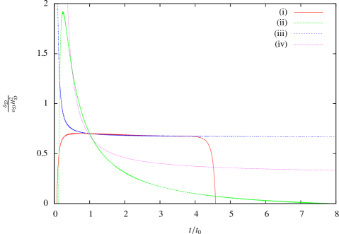
Figure 1: The dimensionless global acceleration parameter $\frac{\ddot{a}_{\mathcal{D}}}{a_{\mathcal{D}}H_{\mathcal{D}}^{2}}$, plotted vs. time (in units of $t/t_{0}$ with $t_{0}$ being the current age of the universe ). The parameter values used are: (i) $\alpha=0.995$, $\beta=0.5$, (ii) $\alpha=0.995$, $\beta=0.5,$ (iii) $\alpha=1.02$, $\beta=0.66$, (iv) $\alpha=1.02$, $\beta=0.66$. (The curves (i) and (iii) correspond to the case when an event horizon is included in the analysis in Section 4).

Following the Buchert framework buchert1 ; weigand as discussed above, the global domain $\mathcal{D}$ is divided into a collection of overdense regions $\mathcal{M}=\cup_{j}\mathcal{M}^{j}$, with total volume $|\mathcal{M}|_{g}=\sum_{j}|\mathcal{M}^{j}|_{g}$ , and underdense regions $\mathcal{E}=\cup_{j}\mathcal{E}^{j}$ with total volume $|\mathcal{E}|_{g}=\sum_{j}|\mathcal{E}^{j}|_{g}$. Assuming that the scale-factors of the regions $\mathcal{E}^{j}$ and $\mathcal{M}^{j}$ are, respectively, given by $a_{\mathcal{E}_{j}}=c_{\mathcal{E}_{j}}t^{\alpha}$ and $a_{\mathcal{M}_{j}}=c_{\mathcal{M}_{j}}t^{\beta}$ where $\alpha$, $\beta$, $c_{\mathcal{E}_{j}}$ and $c_{\mathcal{M}_{j}}$ are constants, one has

$$a_{\mathcal{E}}^{3}=c_{\mathcal{E}}^{3}t^{3\alpha};\>\>\>a_{\mathcal{M}}^{3}=c_{\mathcal{M}}^{3}t^{3\beta}$$ (17)

where $c_{\mathcal{E}}^{3}=\frac{\sum_{j}c_{\mathcal{E}_{j}}^{3}|\mathcal{E}_{i}^{j}|_{g}}{|\mathcal{E}_{i}|_{g}}$ is a new constant, and similarly for $c_{\mathcal{M}}$. The volume fraction of the subdomain $\mathcal{M}$ is given by $\lambda_{\mathcal{M}}=\frac{|\mathcal{M}|_{g}}{|\mathcal{D}|_{g}}$, which can be rewritten in terms of the corresponding scale factors as $\lambda_{\mathcal{M}}=\frac{a_{\mathcal{M}}^{3}|\mathcal{M}_{i}|_{g}}{a_{\mathcal{D}}^{3}|\mathcal{D}_{i}|_{g}}$. We therefore find that the global acceleration equation (14) becomes

$$\frac{\ddot{a}_{\mathcal{D}}}{a_{\mathcal{D}}} = \frac{g_{\mathcal{M}_{h}}^{3}t^{3\beta}}{a_{\mathcal{D}}^{3}}\frac{\beta(\beta-1)}{t^{2}}+\left(1-\frac{g_{\mathcal{M}_{h}}^{3}t^{3\beta}}{a_{\mathcal{D}}^{3}}\right)\frac{\alpha(\alpha-1)}{t^{2}}$$ (18)

$$+2\frac{g_{\mathcal{M}_{h}}^{3}t^{3\beta}}{a_{\mathcal{D}}^{3}}\left(1-\frac{g_{\mathcal{M}_{h}}^{3}t^{3\beta}}{a_{\mathcal{D}}^{3}}\right)\left(\frac{\beta}{t}-\frac{\alpha}{t}\right)^{2}$$

where $g_{\mathcal{M}_{h}}^{3}=\frac{\lambda_{\mathcal{M}_{0}}a_{\mathcal{D}_{0}}^{3}}{t_{0}^{3\beta}}$ is a constant. We obtain numerical solutions of the above equation for various parameter values (see curves (ii) and (iv) of Fig.1). The expansion factor $\beta$ for the overdense subdomain (wall) is chosen to lie between $1/2$ and $2/3$ (since the expansion is assumed to be faster than in the radiation dominated case, and is upper limited by the value for matter dominated expansion).

Note here that using our ansatz for the subdomain scale factors given by Eq.(17), one may try to determine the global scale factor through Eq.(12). In order to do so, one needs to know the inital volume fractions $\lambda_{\ell_{i}}$ which are in turn related to the $c_{\mathcal{E}}$ and $c_{\mathcal{M}}$. However, in our approach based upon the Buchert framework buchert1 ; buchert2 ; weigand we do not need to determine $c_{\mathcal{E}}$ and $c_{\mathcal{M}}$, but in stead, obtain from Eq.(18) the global scale factor numerically by the method of recursive iteration, using the value $\lambda_{\mathcal{M}_{0}}=0.09$ determined through numerical simulations in the earlier literature weigand . We later compare these solutions for the global scale factor with the solutions of the model with an explicit event horizon studied in Section 4.

3.1 Backreaction and Scalar Curvature

It is of interest to study separately the behaviour of the backreaction term in the Buchert model buchert1 ; weigand . The backreaction $\mathcal{Q}_{\mathcal{D}}$ is obtained from (4) to be

$$\mathcal{Q}_{\mathcal{D}}=3\frac{\ddot{a}_{\mathcal{D}}}{a_{\mathcal{D}}}+4\pi G\left\langle\rho\right\rangle_{\mathcal{D}}$$ (19)

Note that we are not considering the presence of any cosmological constant $\Lambda$ as shown in (4). We can assume that $\left\langle\rho\right\rangle_{\mathcal{D}}$ behaves like the matter energy density, i.e. $\left\langle\rho\right\rangle_{\mathcal{D}}=\frac{c_{\rho}}{a_{\mathcal{D}}^{3}}$, where $c_{\rho}$ is a constant. Now, observations tell us that the current matter energy density fraction (baryonic and dark matter) is about 27% and that of dark energy is about 73%. Assuming the dark energy density to be of the order of $10^{-48}\left(GeV\right)^{4}$, we get $\rho_{\mathcal{D}_{0}}\backsimeq 3.699\times 10^{-49}\left(GeV\right)^{4}$. Thus, using the values for the global acceleration computed numerically, the future evolution of the backreaction term $\mathcal{Q}_{\mathcal{D}}$ can also be computed (see curves (ii) and (iv) of Fig.2, where we have plotted the backreaction density fraction $\Omega_{\mathcal{Q}}^{\mathcal{D}}=-\frac{\mathcal{Q}_{\mathcal{D}}}{6H_{\mathcal{D}}^{2}}$). Once we compute the backreaction it is straightforward to calculate the scalar curvature $\mathcal{\left\langle R\right\rangle}_{\mathcal{D}}$ as

$$\mathcal{\left\langle R\right\rangle}_{\mathcal{D}}=16\pi G\left\langle\rho\right\rangle_{\mathcal{D}}-\mathcal{Q}_{\mathcal{D}}-6H_{\mathcal{D}}^{2}$$ (20)

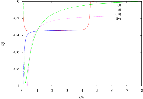
Figure 2: Global backreaction density fraction vs. time. The parameter values used are the same as in Fig. 1.

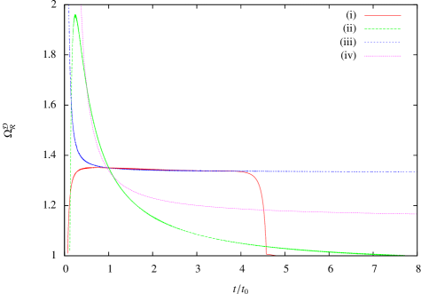
Figure 3: Global scalar curvature density fraction, $\Omega_{\mathcal{R}}^{\mathcal{D}}$ plotted vs. time. The parameter values for curves (i) and (ii) are $\alpha=0.995$, $\beta=0.5$ , and for curves (iii) and (iv) are $\alpha=1.02$, $\beta=0.66$.

3.2 Effective Equation of State

To point out the analogy with the Friedmann equations one may write (4) and (5) as

$$3\frac{\ddot{a}_{\mathcal{D}}}{a_{\mathcal{D}}} = -4\pi G\left(\rho_{eff}^{\mathcal{D}}+3p_{eff}^{\mathcal{D}}\right)$$

$$3H_{\mathcal{D}}^{2} = 8\pi G\rho_{eff}^{\mathcal{D}}$$ (21)

where the effective energy density and pressure are defined as

$$\rho_{eff}^{\mathcal{D}} = \left\langle\rho\right\rangle_{\mathcal{D}}-\frac{1}{16\pi G}\mathcal{Q}_{\mathcal{D}}-\frac{1}{16\pi G}\mathcal{\left\langle R\right\rangle}_{\mathcal{D}}$$

$$p_{eff}^{\mathcal{D}} = -\frac{1}{16\pi G}\mathcal{Q}_{\mathcal{D}}+\frac{1}{48\pi G}\mathcal{\left\langle R\right\rangle}_{\mathcal{D}}$$ (22)

Note that as in (19), here also we are not considering the presence of any cosmological constant $\Lambda$. In this sense, $\mathcal{Q}_{\mathcal{D}}$ and $\mathcal{\left\langle R\right\rangle}_{\mathcal{D}}$ may be combined to some kind of dark fluid component that is commonly referred to as $X$-matter. One quantity characterizing this $X$-matter is its equation of state given by

$$w_{\Lambda,eff}^{\mathcal{D}}=\frac{p_{eff}^{\mathcal{D}}}{\rho_{eff}^{\mathcal{D}}-\left\langle\rho\right\rangle_{\mathcal{D}}}=\frac{\mathcal{Q}_{\mathcal{D}}-\frac{1}{3}\mathcal{\left\langle R\right\rangle}_{\mathcal{D}}}{\mathcal{Q}_{\mathcal{D}}+\mathcal{\left\langle R\right\rangle}_{\mathcal{D}}}=\frac{\Omega_{\mathcal{Q}}^{\mathcal{D}}-\frac{1}{3}\Omega_{\mathcal{R}}^{\mathcal{D}}}{\Omega_{\mathcal{Q}}^{\mathcal{D}}+\Omega_{\mathcal{R}}^{\mathcal{D}}}$$ (23)

which is an effective one due to the fact that backreaction and curvature give rise to effective energy density and pressure. We again plot this effective equation of state by computing its value numerically (see curves (ii) and (iv) of Fig.4), and in the next Section we compare the results with those obtained by considering the effect of an event horizon.

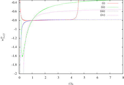
Figure 4: Effective equation of state vs. time. The parameter values used are: (i) $\alpha=0.995$, $\beta=0.5$, (ii) $\alpha=0.995$, $\beta=0.5,$ (iii) $\alpha=1.02$, $\beta=0.66$, (iv) $\alpha=1.02$, $\beta=0.66$

4 Effect of event horizon

In the previous section we have performed a detailed analysis of the future evolution of an accelerating universe by calculating the effect of backreaction from inhomogeneities on the various dynamical quantities within the context of the Buchert framework. As mentioned earlier, an accelerated expansion dictates the formation of an event horizon, and our earlier analysis may be interpreted as a tacit assumption of a horizon scale being set by the scale of homogeneity labelled by the global scale-factor, i.e. $r_{h}\approx a_{\mathcal{D}}$. In the present section we introduce explicitly such an event horizon. Given that we are undergoing a stage of acceleration since transition from an era of structure formation, our aim here is to explore the subsequent evolution of the Universe due to the effects of backreaction in presence of the cosmic event horizon. We can write the equation of the event horizon $r_{h}$, to a good approximation by

$$r_{h}=a_{\mathcal{D}}\int_{t}^{\infty}\frac{dt^{\prime}}{a_{\mathcal{D}}(t^{\prime})}$$ (24)

Note that though, in general, spatial and light cone distances and corresponding accelerations could be different, as shown explicitly in the framework of Lemaitre–Tolman–Bondi (LTB) models bolejko , an approximation for the event horizon which forms at the onset of acceleration could be defined in the way above in the same spirit as $a_{\mathcal{D}}=c_{F}a_{F}$. The concept of the event horizon just ensures that the effect of backreactions are computed by taking into account only the causally connected processes, but leaving out the processes that are not causally connected, i.e., the effect of inhomogeneities from regions that lie outside the event horizon. Now, from its very definition the event horizon is observer dependent. For example, the event horizon for an observer ‘A’ based, say, in our group of local galaxies, is different from the event horizon for another hypothetical observer ‘B’ based, say, somewhere in a very distant region of the universe. This means that certain regions in the universe that are causally connected to ‘A’ may not be connected to ‘B’, and vice-versa. The regions not causally connected to ‘A’ have no impact on the physics, i.e., the spacetime metric for ‘A’ is unaffected by the backreaction from inhomogeneities at those regions. Hence, in a two scale void-wall model that we are using, the event horizon has to be chosen with respect to either ‘A’ (say, wall), or ‘B’ (say, void). However, the important assumption here is that there is indeed a scale of global homogeneity which lies within the horizon volume, and the physics is translationally invariant over such large scales. The void-wall symmetry of Eq.(14) thereby ensures that the conclusions are similar whether one chooses to define the event horizon with respect to the wall or with respect to the void.

Since an event horizon forms, only those regions of $\mathcal{D}$ that are within the event horizon are causally accessible to us. We hence define a new fiducial global domain as that contained within the horizon, which naturally is smaller than the original global domain that we dealt with in our earlier equations. We assume that the entire Buchert formalism, as outlined in Section 2 holds in this new global domain. Note that even if conservation of total rest mass is not strictly or exactly obeyed inside this fiducial global domain, the magnitude of violation is assumed to be rather small since the volume and mass contained within the event horizon is huge, and inflow or outflow is assumed to be a rather insignificant fraction of the total amount. Therefore, in our subsequent analysis we work under the assumption that the Buchert framework is valid up to this approximation. Denoting this domain as $\widetilde{\mathcal{D}}$ and the corresponding volume as $\left|\widetilde{\mathcal{D}}\right|_{g}$, the volume scale-factor is defined as

$$a_{\widetilde{\mathcal{D}}}^{3}=\frac{\left|\widetilde{\mathcal{D}}\right|_{g}}{\left|\widetilde{\mathcal{D}}_{i}\right|_{g}}=\frac{\frac{4}{3}\pi r_{h}^{3}}{\left|\widetilde{\mathcal{D}}_{i}\right|_{g}}$$ (25)

where $\left|\widetilde{\mathcal{D}}_{i}\right|_{g}$ is the volume of the fiducial global domain at some initial time, which we can take to be the time when the transition from deceleration to acceleration occurs. The average of a scalar valued function (eq. (7)) in $\widetilde{\mathcal{D}}$ will be written as

$$\left\langle f\right\rangle{}_{\mathcal{\widetilde{D}}}(t)=\frac{\int_{\mathcal{\widetilde{D}}}f(t,X^{1},X^{2},X^{3})d\mu_{g}}{\int_{\mathcal{\widetilde{D}}}d\mu_{g}}=|\mathcal{\widetilde{D}}|_{g}^{-1}\int_{\mathcal{\widetilde{D}}}fd\mu_{g}$$ (26)

The Einstein equations (4), (5)and (6) are also assumed to hold in this new domain, after we replace $\mathcal{D}$ with $\widetilde{\mathcal{D}}$ in the equations. The domain $\widetilde{\mathcal{D}}$ is considered to be divided into several subregions and the average of the scalar valued function $f$ on the domain $\mathcal{\widetilde{D}}$ may then be split into the averages of $f$ on the subregions $\mathcal{\widetilde{F}}_{\ell}$ in the form,

$$\left\langle f\right\rangle_{\mathcal{\widetilde{D}}}=\underset{\ell}{\sum}|\mathcal{\widetilde{D}}|_{g}^{-1}\underset{\alpha}{\sum}\int_{\mathcal{\widetilde{F}}_{\ell}^{(\alpha)}}fd\mu_{g}=\underset{\ell}{\sum}\lambda_{\ell}\left\langle f\right\rangle_{\mathcal{\widetilde{F}}_{\ell}}$$ (27)

where $\lambda_{\ell}=|\mathcal{\widetilde{F}}_{\ell}|_{g}/|\mathcal{\widetilde{D}}|_{g}$, is the volume fraction of the subregion $\mathcal{\widetilde{F}}_{\ell}$. Just like in Section 3 here also we consider the global domain $\widetilde{\mathcal{D}}$ to be divided into a collection of overdense regions $\mathcal{M}=\cup_{j}\mathcal{M}^{j}$, with total volume $|\mathcal{M}|_{g}=\sum_{j}|\mathcal{M}^{j}|_{g}$ , and underdense regions $\mathcal{E}=\cup_{j}\mathcal{E}^{j}$ with total volume $|\mathcal{E}|_{g}=\sum_{j}|\mathcal{E}^{j}|_{g}$. We also assume that the scale-factors of the regions $\mathcal{E}$ and $\mathcal{M}$ are, respectively, given by $a_{\mathcal{E}}=c_{\mathcal{E}}t^{\alpha}$ and $a_{\mathcal{M}}=c_{\mathcal{M}}t^{\beta}$ where $\alpha$, $\beta$, $c_{\mathcal{E}}$ and $c_{\mathcal{M}}$ are constants. The volume fraction of the subdomain $\mathcal{M}$ is given by $\lambda_{\mathcal{M}}=\frac{|\mathcal{M}|_{g}}{|\mathcal{\widetilde{D}}|_{g}}$, which can be rewritten in terms of the corresponding scale factors as $\lambda_{\mathcal{M}}=\frac{a_{\mathcal{M}}^{3}|\mathcal{M}_{i}|_{g}}{a_{\widetilde{\mathcal{D}}}^{3}|\widetilde{\mathcal{D}}_{i}|_{g}}$.

We can then find the acceleration of this fiducial global domain $\widetilde{\mathcal{D}}$, just like we did in Section 3. So in this case the global acceleration for $\widetilde{\mathcal{D}}$ is given by

$$\frac{\ddot{a}_{\mathcal{\widetilde{\mathcal{D}}}}}{a_{\widetilde{\mathcal{D}}}} = \frac{\widetilde{c}_{\mathcal{M}}^{3}t^{3\beta}}{a_{\widetilde{\mathcal{D}}}^{3}}\frac{\beta(\beta-1)}{t^{2}}+\left(1-\frac{\widetilde{c}_{\mathcal{M}}^{3}t^{3\beta}}{a_{\widetilde{\mathcal{D}}}^{3}}\right)\frac{\alpha(\alpha-1)}{t^{2}}$$ (28)

$$+2\frac{\widetilde{c}_{\mathcal{M}}^{3}t^{3\beta}}{a_{\widetilde{\mathcal{D}}}^{3}}\left(1-\frac{\widetilde{c}_{\mathcal{M}}^{3}t^{3\beta}}{a_{\widetilde{\mathcal{D}}}^{3}}\right)\left(\frac{\beta}{t}-\frac{\alpha}{t}\right)^{2}$$

But we can see from (25) that $a_{\widetilde{\mathcal{D}}}\propto r_{h}$, so we can write $\frac{\ddot{a}_{\mathcal{\widetilde{\mathcal{D}}}}}{a_{\widetilde{\mathcal{D}}}}=\frac{\ddot{r}_{h}}{r_{h}}$ and hence the above equation can be written as

$$\frac{\ddot{r}_{h}}{r_{h}} = \frac{c_{\mathcal{M}_{h}}^{3}t^{3\beta}}{r_{h}^{3}}\frac{\beta(\beta-1)}{t^{2}}+\left(1-\frac{c_{\mathcal{M}_{h}}^{3}t^{3\beta}}{r_{h}^{3}}\right)\frac{\alpha(\alpha-1)}{t^{2}}$$ (29)

$$+2\frac{c_{\mathcal{M}_{h}}^{3}t^{3\beta}}{r_{h}^{3}}\left(1-\frac{c_{\mathcal{M}_{h}}^{3}t^{3\beta}}{r_{h}^{3}}\right)\left(\frac{\beta}{t}-\frac{\alpha}{t}\right)^{2}$$

Note here that the global domain $\widetilde{\mathcal{D}}$ is a fiducial one defined with respect to the observer-dependent event horizon for the purpose of our intermediate analysis, and ultimately we are interested to obtain the evolution of the global domain $\mathcal{D}$. In order to get the acceleration of the global domain $\mathcal{D}$ we first convert (24) to a differential form,

$$\dot{r_{h}}=\frac{\dot{a}_{\mathcal{D}}}{a_{\mathcal{D}}}r_{h}-1$$ (30)

Thus, the evolution of the scale-factor $a_{\mathcal{D}}$ is now governed by the set of coupled differential equations (30) and (29). We numerically integrate these equations by using as an ‘initial condition’ the observational constraint $q_{0}=-0.7$, where $q_{0}$ is the current value of the deceleration parameter. The global acceleration obtained from these equations is plotted in Fig. 1 (curves (i) and (iii)). The expression for $q_{0}$ is a completely analytic function of $\alpha$, $\beta$ and $t_{0}$, but we since we are studying the effect of inhomogeneities therefore the Universe cannot strictly be described based on a FRW model and hence the current age of the Universe ($t_{0}$) cannot be fixed based on current observations which use the FRW model to fix the age. Instead for each combination of values of the parameters $\alpha$ and $\beta$ we find out the value of $t_{0}$ for our model from (28) by taking $q_{0}=0.7$. Note that we use the same technique for finding $t_{0}$ in Section 3, where we use (18).

5 Discussions

Let us now compare the nature of acceleration of the Universe for the two models described respectively, in Sections 3 and 4. The global acceleration for the two models have been plotted in Fig. 1. Here curves (i) and (iii) are for the case when an event horizon is included, and curves (ii) and (iv) correspond to the case without an event horizon. For $\alpha<1$ the acceleration becomes negative in the future for both the cases. The acceleration reaches a much greater value when no event horizon is present and that too very quickly, but decreases much more gradually than when an event horizon is included. This behaviour could be due to the fact that the inclusion of the event horizon somehow limits the global volume of domain $\mathcal{D}$ in such a way that the available volume of the underdense region $\mathcal{E}$ is lesser than when an event horizon is not included. This causes the overdense region $\mathcal{M}$ to start dominating much earlier and thus causing global deceleration much more quickly. When $\alpha>1$ the acceleration decreases and reaches a positive constant value asymptotically when an event horizon is not included (curve (iv)), and also when it is included (curve (iii)). Here also we can see that when we include an event horizon in our calculations then there is much more rapid deceleration, the reason for which is mentioned above. Initially the curves for the two cases are almost identical qualitatively, but later on they diverge due to the faster deceleration for the case when an event horizon is included.

A similar comparison of the backreaction for the two models is presented in Fig. 2. From the expression of $\Omega_{\mathcal{Q}}^{\mathcal{D}}$ and (8) it can be seen that the backreaction will be dominated by the variance of the local expansion rate $\theta$. Here we observe that even for the model where an event horizon is not included, $\Omega_{\mathcal{Q}}^{\mathcal{D}}$ is negative for the duration over which the acceleration is positive. For $\alpha<1$ the backreaction density first reaches a minimum and then keeps on rising. For the case where an event horizon is included (curve (i)) the backreaction density remains almost contant after reaching a minimum but then when it rises it does so very rapidly as compared to the case where an even thorizon is not included (curve (ii)). For $\alpha>1$ the backreaction density keeps on rising monotonically. Here curves for both the models are initially very similar qualitatively but later on they diverge.

When we look at Fig. 3, where the scalar curvature density has been plotted we observe that the scalar curvature turns out to be negative for the duration when the Universe is in accelerated phase, which is what we expect from our knowledge of FRW cosmology. For $\alpha<1$ the curvature density increases to a maximum and then decreases, the rise to the maximum being much more fast for the case where an event horizon is not included (curve (ii)) whereas the fall from the maximum being much more fast for the case where the event horizon is included (curve (i)). For $\alpha>1$ the curvature density keeps on decreasing monotonically for both the cases.

We next consider the effective equation of state $w_{\Lambda,eff}^{\mathcal{D}}$ (Fig. 4). It remains negative for the entire duration over which the acceleration is positive. For $\alpha<1$, $w_{\Lambda,eff}^{\mathcal{D}}$ first reaches a minimum and then keeps on rising. The falling to the minimum is much faster for the model where an event horizon is not included (curve (ii)) whereas for the case with an event horizon the equation of state remains almost constant after reaching the minimum but then rises very rapidly (curve(i)). For $\alpha>1$ the curves for the two cases are very similar initially qualitatively (again like backreaction plots) but later on they diverge.

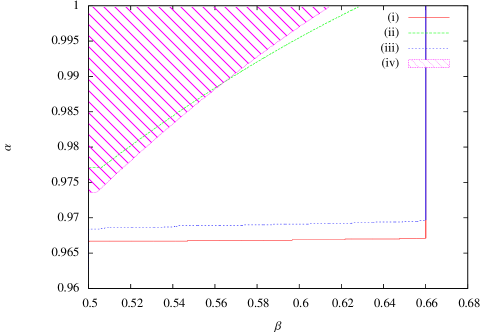
Figure 5: The range of parameters $\alpha$ and $\beta$ for which future deceleration takes place, shown within the respective contours for the curves (i) and (iii) corresponding to the case with an event horizon, and the curves (ii) and (iv) corresponding to the case where an event horizon is not considered. The value of $\lambda_{\mathcal{M}_{0}}$ for the curves (i) and (ii) is $0.15$ and for curves (iii) and (iv) is $0.2$. The shaded region corresponds to the curve (iv) demarcating the parameter space for this case when acceleration vanishes in finite future time.

From our analysis so far it is clear that the acceleration of the Universe could become negative in the future for certain values of the parameters $\alpha$ and $\beta$, which represent the growth rates of the scale factors corresponding to the void and wall, respectively. The range of values of $\alpha$ and $\beta$ for which a future transition to deceleration is possible, is depicted in Fig. 5. We provide a contour plot of $\alpha$ versus $\beta$ demarcating the range in parameter space (inside of the contours) for which acceleration vanishes in finite future time. We see that the curves for the model with an event horizon (curves (i) and (iii)) have the almost the same value of $\alpha$ for various values of $\beta$. This shows that for this case there is no dependence on the value of $\beta$ to make the acceleration negative in the future. For the case where there is no event horizon (curves (ii) and (iv)), initially the values of $\alpha$ are the same for various values of $\beta$, but later on the values of $\alpha$ begin to change and increases as $\beta$ increases. Since the acceleration has no chance of becoming negative when we have $\alpha>1$, therefore the maximum limit of $\alpha$ for all the cases is depicted by the line $\alpha=1$.

6 Conclusions

To summarize, in this work we have performed a detailed analysis of the various aspects of the future evolution of the presently accelerating universe in the presence of matter inhomogeneities. The backreaction of inhomogeneities on the global evolution is calculated within the context of the Buchert framework for a two-scale non-interacting void-wall model buchert1 ; buchert2 ; buchert3 ; weigand . We first analyze the future evolution using the Buchert framework by computing various dynamical quantities such as the global acceleration, strength of backreaction, scalar curvature and equation of state. Though in this case we do not consider explicitly the effect of the event horizon, it may be argued that a horizon scale is implicitly set by the scale of global homogeneity labelled by the global scale-factor. We show that the Buchert framework allows for the possibility of the global acceleration vanishing at a finite future time, provided that none of the subdomains accelerate individually (both $\alpha$ and $\beta$ are less than $1$).

We next consider in detail a model with an explicit event horizon, first presented in bose . The observed present acceleration of the universe dictates the occurrence of a future event horizon since the onset of the present accelerating era. It may be noted that though the event horizon is observer dependent, the symmetry of the equation (14) ensures that our analysis would lead to similar conclusions for a ‘void’ centric observer, as it does for a ‘wall’ centric one. In bose we had shown that the presence of the cosmic event horizon causes the acceleration to slow down significantly with time. In the present paper in order to understand better the underlying physics behind the slowing down of the global acceleration, we have explored the nature of the global backreaction, scalar curvature and effective equation of state. We have then provided a quantitative comparison of the evolution of these dynamical quantities of this model with the case when an event horizon is not included.

The approach of incorporating the effects of the event horizon in the present paper is different from that used in bose . Here we start with the assumption that the portion of the global domain enclosed by the event horizon is a fiducial domain in which the original Buchert equations are shown to hold. We have then calculated the acceleration of this fiducial domain using the Buchert equations. Finally, we have utilized a relation between the event horizon and the scale factor of the global domain to find out the acceleration of the original global domain. In contrast, in bose we had explored the effect of the event horizon by assuming that the global domain was cut off by the horizon, thus leading to apparent volume fractions which we could observe. We then used these apparent volume fractions in the Buchert acceleration equation to find the global acceleration, effectively modifying the original Buchert equation. The main prediction of possible future deceleration remains the same using both these approaches, though with certain quantitative differences in the rate of deceleration. The present analysis also clarifies that the prediction of future deceleration may not be solely attributable to the event horizon, but may also follow purely within the Buchert model under certain conditions.

Our analysis shows that, in comparison with the model without an event horizon, during the subsequent future evolution the global acceleration decreases more quickly at late times when we include an event horizon. The reason for this effect is that in the latter model an effective reduction of the volume fraction for the void leads to the overdense region starting to dominate much earlier and hence, causes faster deceleration of the universe. We also found that the acceleration does not vanish in finite time, but in stead goes asymptotically to a constant value for $\alpha>1$ for both the cases. Nonetheless, when $\alpha>1$, the curves for acceleration, backreaction, scalar curvature, and effective equation of state for both the cases are very similar qualitatively and only diverge later on. We finally demarcate the region in the parameter space of the growth rates of the void and the wall, where it is possible to obtain a transition to deceleration in the finite future.

Our results indicate the fascinating possibility of backreaction being responsible for not only the present acceleration as shown in earlier works rasanen1 ; weigand , but also leading to a transition to another decelerated era in the future. Another possibility following from our analysis is of the Universe currently accelerating due to a different mechanism sahni , but with backreaction buchert1 ; buchert3 ; weigand later causing acceleration to slow down. Finally, it may be noted that the formalism for obtaining backreaction buchert1 ; buchert2 ; buchert3 ; weigand used here relies on averaging on constant time hypersurfaces, and incorporating effects based on causality within this framework may be open to criticism. A framework more suitable for exploring such effects could be a procedure based on light-cone averaging that has been proposed recently gasperini . Though the full implications on the cosmological scenario of the latter framework are yet to be deduced, our analysis of including the effect of the event horizon introduces certain elements of lightcone physics in the study of the role of backreaction from inhomogeneities on the global cosmological evolution. The present analysis may be viewed as an attempt to superimpose the effect of the event horizon on the Buchert framework, and explore if certain interesting results could be obtained that are at least qualitatively reliable. These predictions could be open for scrutiny as and when a rigorous formalism is developed to deal with such effects.

References

- (1) S. Perlmutter, et. al., Nature 391, 51 (1998); A. G. Riess et. al., Ap. J. 116, 1009 (1998); M. Hicken et al., ApJ, 700, 1097 (2009); M. Seikel, D. J. Schwarz, JCAP 02, 024 (2009).
- (2) S. Weinberg, Rev. Mod. Phys., 61, 1 (1989); T. Padmanabhan, Adv. Sci. Lett. 2, 174 (2009).
- (3) V. Sahni, in Papantonopoulos E., ed., Lecture Notes in Physics Vol. 653, The Physics of the Early Universe. Springer, Berlin, p. 141 (2004); E. J. Copeland, M. Sami, and S. Tsujikawa, Int. J. Mod. Phys. D 15, 1753 (2006).
- (4) M. Seikel, D. J. Schwarz, J. Cosmol. Astropart. Phys., 02, 024 (2009)
- (5) R. Zalaletdinov, Gen. Rel. Grav., 24, 1015 (1992); Gen. Rel. Grav., 25, 673 (1993).
- (6) T. Buchert, Gen. Rel. Grav., 32, 105 (2000); T. Buchert, Gen. Rel. Grav. 33, 1381. (2001).
- (7) T. Buchert, M. Carfora, Phys. Rev. Lett. 90, 031101 (2003).
- (8) E. W. Kolb, S. Matarrese, A. Notari and A. Riotto, Phys. Rev. D 71, 023524 (2005).
- (9) M. Gasperini, G. Marozzi, G. Veneziano, J. Cosmol. Astropart. Phys. 0903, 011 (2009); ibid. 1002, 009 (2010); M. Gasperini, G. Marozzi, F. Nugier, G. Veneziano, J. Cosmol. Astropart. Phys. 1107, 008 (2011); I. Ben-Dayan, M. Gasperini, G. Marozzi, F. Nugier, G. Veneziano, J. Cosmol. Astropart. Phys. 04, 036 (2012).
- (10) S. Räsänen, J. Cosmol. Astropart. Phys., 0402, 003 (2004); S. Räsänen, J. Cosmol. Astropart. Phys., 0804, 026 (2008); S. Räsänen, J. Cosmol. Astropart. Phys., 02, 011 (2009); S. Räsänen, Phys. Rev. D 81, 103512 (2010).
- (11) D. L. Wiltshire, New J. Phys. 9, 377 (2007); D. L. Wiltshire, Phys. Rev. Lett. 99, 251101 (2007).
- (12) I. Ben-Dayan, M. Gasperini, G. Marozzi, F. Nugier, G. Veneziano, Phys. Rev. Lett. 110, 021301 (2013).
- (13) W. Valkenburg, M. Kunz and C. Clarkson, arXiv: 1302.6588.
- (14) W. Valkenburg, V. Marra and C. Clarkson, arXiv: 1209.4078.
- (15) P. Fleury, H. Dupuy and J.-P. Uzan, Phys. Rev. D 87, 123526 (2013).
- (16) A. Ishibashi, R. M. Wald, Classical Quantum Gravity, 23, 235 (2006).
- (17) A. Paranjape, T. P. Singh, Phys. Rev. D 78, 063522 (2008); T. P. Singh, arXiv:1105.3450.
- (18) E. W. Kolb, S. Marra, S. Matarrese, Phys. Rev. D, 78, 103002 (2008).
- (19) M. Mattsson, T. Mattsson, J. Cosmol. Astropart. Phys. 10, 021 (2010).
- (20) T. Buchert, M. Carfora, Class. Quant. Grav. 25, 195001 (2008).
- (21) A. Wiegand, T. Buchert, Phys. Rev. D 82, 023523 (2010).
- (22) N. Bose, A. S. Majumdar, MNRAS Letters 418, L45 (2011).
- (23) K. Bolejko, L. Andersson, J. Cosmol. Astropart. Phys. 10, 003 (2008).