Statistical analysis of dwarf galaxies and their globular clusters in the Local Volume

Abstract

Morphological classification of dwarf galaxies into early and late type, though can account for some of their origin and characteristics but does not help to study their formation mechanism. So an objective classification using Principal Component analysis together with K means Cluster Analysis of these dwarf galaxies and their globular clusters is carried out to overcome this problem. It is found that the classification of dwarf galaxies in the Local Volume is irrespective of their morphological indices. The more massive ($M_{V0}<-13.7$) galaxies evolve through self-enrichment and harbor dynamically less evolved younger globular clusters (GCs) whereas fainter galaxies ($M_{V0}>-13.7$) are influenced by their environment in the star formation process.
Key words: methods - statistical analysis: dwarf galaxies- globular clusters

1 Introduction

The galaxies with low luminosities, low metallicities having smaller sizes are termed as dwarf galaxies. Study of dwarf galaxies is important as massive galaxies are supposed to be formed by hierarchical merging of dwarf galaxies during the evolution of early Universe (White & Rees 1978; Geisler et al. 2007; Haines et al. 2006). Such objects lose gas easily due to their shallow potential wells. Low surface brightness (LSB) dwarf galaxies are classified primarily into three groups : early type ( dwarf spheroidal, dSph, and dwarf elliptical, dE), late type (dwarf irregular, dIrr), and transition type galaxies (Kormendy 1985; Karachentseva et al. 1985; Grebel 1999). There is no sharp boarder line between these morphological types (see e.g. Sharina et al. 2008 and references therein, hereafter: S08). Also population gradients exist in early-type dwarf galaxies, and dSphs and dIrrs have exponential surface brightness profiles. All these facts indicate that classification, based on morphology and stellar content is not sufficient to study the formation and evolutionary status of these objects. A more sophisticated classification is essential for studying true formation mechanisms of this class of objects. However the objects under consideration share one common property. They all harbor globular clusters those are older than several Gyr which indicates that early globular cluster formation took place irrespective of the morphological type. So these globular clusters can serve as unique tool to investigate the chemical evolution of the host galaxies. Hence a proper classification of globular clusters in LSB galaxies is necessary for finding information regarding star formation histories in these dwarf galaxies which is important input for studying galaxy formation mechanism. Since Hubble (1922, 1926) tunning fork diagram, very little attempts have been taken on development of an objective classification for normal and dwarf galaxies using statistical methods and principles (Whitmore 1984; Vaduvescu & McCall 2005; Fraix Burnet et al. 2006; Chattopadhyay & Chattopadhyay 2006; van den Bergh 2007; van den Bergh 2008; Woo et al. 2008) though few works have been carried out on dE classification and formation scenarios (Marin-Franch & Aparicio 2002; Lisker et al. 2007; Penny & Conselice 2008) in Virgo, Perseus and Coma clusters of galaxies which is again the consideration of a particular morphological type and therefore not exhaustive. In order to identify the parameters those are mostly responsible for the variation among the dwarf galaxies and their globular clusters and to classify them into homogeneous groups for searching the possible formation mechanism we have to use some statistical techniques like Principal Component Analysis (PCA) and Cluster Analysis (CA).

In the present paper, in order to study the underlying features of the dwarf galaxy population we have used statistical methods like PCA, CA and Discriminant analysis. By treating the samples under consideration as representatives of the corresponding underlying population of dwarf galaxies , these methods help us to make inference regarding the above mentioned population ( and not only for the samples under consideration). As a result, on the basis of the present study we can make some general conclusions which are not feasible on the basis of visual studies.

In Section 2 the data sets are discussed. The methods, used, are described in Section 3 while results, discussions and conclusions are summarized in Sections 4, 5 and 6 respectively.

2 Data Set

Our analysis is based on two data sets of dwarf galaxies and their globular clusters (GCs) in the Local Volume (LV).
Data set 1
This consists of 60 dwarf galaxies taken from a data set of 104 dwarf galaxies (Sharina et al. 2008) (Table 1). The parameters considered from Sharina et al. (2008 hereafter S08) are distance modulus ($\mu_{0}$, in mag), morphological index (T), mean metallicity of the red giant branches ([Fe/H], in dex), effective color corrected for extinction($(V-I)_{e0}$, in mag), logarithm of projected major axis from CNG($log(Diam)$, in Kpc), logarithm of limiting diameter ($log(Dlim)$, in Kpc), limiting V and I absolute magnitudes within the diameter Dlim corrected for extinction ($M_{V0},M_{I0}$), extinction corrected mean SB within 25 magnitude isophote in V and I magnitudes ($SBV_{25,0},SBI_{25,0}$ in $magarcsec^{-2}$),effective surface brightness in V band corrected for extinction ($SBV_{e0}$, in $magarcsec^{-2}$), logarithm of effective radius ($log(R_{e})$ in Kpc), logarithm of model exponential scale length ($logh$, in Kpc), best exponential fitting central surface brightness in V and I bands corrected for extinction (SBVC0, SBIC0 in $magarcsec^{-2}$) respectively. The parameters used from Karachentsev et al.(2004, hereafter: CNG) are HI rotational velocity ($V_{m}$ in $Kms^{-1}$), HI mass to luminosity ratio ($M_{HI}/L$ in solar units), and tidal index ($\Theta$). The scaling parameters used from Georgiev et al. (2010) are globular cluster specific frequency ($S_{N}$), specific luminosity ($S_{L}$), specific mass ($S_{M}$), specific number ($\hat{T}$), logarithm of specific GC formation efficiency as a function of galaxy luminosity and mass ($\eta_{L},\eta_{M}$), total stellar mass ($M_{*,V}$ in $10^{7}M_{\odot}$) and HI mass of the host galaxy ($M_{HI}$ in $10^{7}M_{\odot}$) respectively.
During selection of parameters for PCA and CA the following things were taken into consideration.
(i) The parameters must be intrinsic in nature.
(ii) For almost physically similar parameters any one is chosen at random because inclusion of similar parameters are considered as redundant in CA.
(iii) All the parameters should be without missing values as CA does not allow parameters having missing values exceeding 5% for which mean substitution might be allowed (Little & Rubin 2002).
With respect to the above aspects (viz. (i)) we excluded $\mu_{0}$ and T which were not intrinsic properties of dwarfs. We included $SBV_{25,0},SBI_{25,0},M_{V0},M_{I0},logR_{e},logh$. So $SBVL,SBIL,MV_{25},MI_{25},R_{V,25},R_{I,25}$ were not included with respect to (ii). We have not considered remaining parameters except $\Theta$ with respect to (iii) as they have missing values exceeding 5% but once the dwarf galaxies are classified we used them to study their properties in more detail. So among all these parameters only 13 parameters from Sharina et al. (2008)excluding $\mu_{0}$ and T, together with ($\Theta$) from Karachentsev et al.(2004) are directly used for PCA and CA as the sample is without any missing values with respect to these 14 parameters. This is a very standard procedure followed during PCA and CA for a sample of astronomical objects. In order to have a sample where the values of all the parameters corresponding to each dwarf galaxy are available, we had to drop observations corresponding to remaining 44 dwarf galaxies and as a result we get a sample of size 60 from the original one. The sample is not complete as there are many more galaxies in the LV which are yet to be observed. In this sense no catalogue is complete. The question remains whether the sample is a good representative of the original one or not. Regarding this point all the two point correlations discussed in the previous paper (S08) are still in place after the selection of the present sample. It is important, that it contains all transitional type galaxies (dSph/dIrr, T = -1) from the original sample. So all morphological types are well represented in this sense. A list of dwarf galaxies considered in Data set 1 is given in Table 1.

Data set 2
This consists of 100 GCs in the Local Volume dwarf galaxies (Sharina et al. 2005). Three candidates Sc 22-2-879, Sc 22-100 and Sc 22-4-106 were removed as they are identified later as galaxies and not GCs (Da Costa et al. 2009). Also the parameters of the GCs in UGC4115, KK65 and UGC3755 are recalculated using the current distances 7.727, 8.017 and 7.413 Mpc repectively (Tully et al. 2006). The parameter set consists of logarithm of half light radius ($log(r_{h})$ in parsec), apparent axial ratio (e), integrated absolute magnitude (V0, in mag) corrected for extinction, integrated absolute $(V-I)_{0}$ color (corrected for Galactic extinction, in mag), projected distance from the host galaxy ($d_{proj}$, in Kpc), central surface brightness in V and I bands ($\mu_{V0}$, $\mu_{I0}$ in $magarcsec^{-2}$), logarithm of King core radius and tidal radius ( $log(r_{c})$, $log(r_{t})$ in parsec) respectively.

3 Method

Principal Component Analysis (PCA) is a very common technique used in data reduction and interpretation in multivariate analysis. We are interested in discovering which parameters in a data set form coherent subgroups that are relatively independent of each other. The specific aim of the analysis is to reduce a large number of parameters to a smaller number while retaining maximum spread among experimental units. The analysis therefore helps us to determine the optimum set of parameters causing the overall variations in the nature of objects under consideration. PCA has been discussed and used by various authors (Babu et al. 2009; Chattopadhyay & Chattopadhyay 2006, 2007; Whitmore 1984; Murtagh & Heck 1987).

Cluster analysis (CA) is the art of finding groups in data. Over the last forty years different algorithms and computer programs have been developed for CA. The choice of a clustering algorithm depends both on the type of data available and on the particular purpose.

In the present study we have used K- Means partitioning algorithm (MacQueen 1967)for clustering. This method constructs K clusters i.e. it classifies the data into K groups which together satisfy the requirement of a partition such that each group must contain at least one object and each object must belong to exactly one group. So there are at most as many groups as there are objects ($K<=n$). Two different clusters cannot have any object in common and the K groups together add up to the full data set. Partitioning methods are applied if one wants to classify the objects into K clusters where K is fixed (which should be selected optimally). The aim is usually to uncover a structure that is already present in the data. The K- Means is probably the most widely applied partitioning clustering technique.

Here to perform K-means clustering we have used MINITAB package. Under this package cluster centers have been chosen on the basis of group average method which makes the process almost robust. This method has been developed by Milligan (1980).

By using this algorithm we first determined the structures of sub populations (clusters) for varying numbers of clusters taking K=2,3,4 etc. For each such cluster formation we computed the values of a distance measure $d_{K}=(1/p)min_{x}E[(x_{K}-c_{K})^{{}^{\prime}}(x_{K}-c_{K})]$ which is defined as the distance of the $x_{K}$ vector (values of the parameters) from the center $c_{K}$ (which is estimated as the mean value), p is the order of the $x_{K}$ vector. Then the algorithm for determining the optimum number of clusters is as follows (Sugar & James 2003). Let us denote by $d_{K}^{\bf{}^{\prime}}$ the estimate of $d_{K}$ at the $K^{th}$ point. Then $d_{K}^{\bf{}^{\prime}}$ is the minimum achievable distortion associated with fitting K centers to the data. A natural way of choosing the number of clusters is to plot $d_{K}^{\bf{}^{\prime}}$ versus K and look for the resulting distortion curve (Figs.1 & 2, bottom one of each figure). This curve is always monotonic decreasing. Initially one would expect much smaller drops for K greater than the true number of clusters because past this point adding more centers simply partitions within groups rather than between groups. According to Sugar & James (2003), for a large number of items the distortion curve when transformed to an appropriate negative power (p/2), will exhibit a sharp ”jump” (if we plot K versus transformed $d_{K}^{\bf{}^{\prime}}$). Then we calculated the jumps in the transformed distortion as $J_{K}=(d_{K}^{\bf{}^{\prime}-{p/2}}-d_{K-1}^{\bf{}^{\prime}-{p/2}}$).

The optimum number of clusters is the value of K associated with the largest jump. The largest jump can be determined by plotting $J_{K}$ against K and the highest peak will correspond to the largest jump (Figs.1 & 2, top one of each figure).

It is well known that both the methods PCA and CA are parameter dependent and the parameters considered should be responsible for the variation of the objects under consideration. In the present situation all the parameters of that type are taken into consideration. As we have to depend on the available data only, it was not possible for us to consider many unobserved parameters whose inclusion might have improved the classification e.g. inclusion of central velocity dispersion etc. and many more. But the question is, given the parameters and sample whether the classification is robust or not. In this respect a discriminant analysis is performed ( Johnson & Wichern 1998) to verify the acceptability of the classification by computing misclassification probabilities for the different dwarfs and GCs. If the original classification is robust then every dwarf or GC should be classified again as a member of the same class that it was before. Tables 2, 3 show the result of a discriminant analysis.The fractions of correct classifications are 0.983 and 0.97 respectively which imply that the classifications are almost robust. As in the present situation we have only one sample, it is difficult to say whether the same results will be obtained for other samples also. It can only be inferred that if the present sample is a good representative of the underlying population of the dwarf galaxies, then the results obtained in this paper are generally true.

4 Dwarf galaxies of the Local Volume

For PCA, at first we have computed a correlation matrix with all the 14 parameters for Data set 1 and have taken any one of the two physically similar (e.g. absolute magnitudes in V and I bands) highly correlated (correlation $>$ 0.7) parameters. Following this method 8 parameters are selected for PCA. They are $\Theta,[Fe/H],M_{V0},SBV_{25,0},(V-I)_{e0},SBV_{e0},log(R_{e}),logh$ respectively. For these 8 parameters, PCA analysis gives four Principal Components with eigen values greater than or equal to 1 and at the same time almost 87.7 % overall variation. So we have taken these four Principal Components and have computed the correlations of the parameters appearing in each Principal Component with the corresponding Principal Component. We have considered those parameters as significant one for which the correlation is greater than 0.65 as a thumb rule. Thus following this procedure the significant parameters as outcome are $M_{V0},SBV_{e0}$ and $log(R_{e})$ (from the first Principal Component), $\Theta,(V-I)_{e0}$ (from the second one) and $[Fe/H]$(from the third one). Fourth component contribute no parameters with such a high correlation.

For cluster analysis we have taken the above six significant parameters and used the method assuming K = 1,2,3 etc. The optimum number of coherent groups by the above method is obtained at K=2 (viz. G1 and G2). The ’distortion’ and the ’jump’ curves are shown in Fig. 1. The mean values with standard errors for some parameters and significant correlations with their p values are shown in Table 4 for the groups G1 and G2 respectively.

Under the multivariate situation the role of all the parameters are important for classification as they are correlated to each other but sometimes one or two parameters may play a significant role over the others when there are large variations among the values of those parameters. In the present situation the magnitude ($M_{V0}$), tidal index ($\Theta$) and effective surface brightness ($SBV_{e0}$) play such role (Table 3). Although in terms of magnitude it is possible to find a single cut at $M_{V0}=-13.7$ irrespective of the other two (Fig. 3), if we consider Fig. 4 it is clear that no such single cut is available in terms of $\Theta$. As such the classification is based mainly on the three major parameters $M_{V0},\Theta$ and $SBV_{e0}$ and not only the magnitude. In such multivariate set up we discuss the marginal situations (i.e. the effect of some single parameter) in order to display the results graphically so that one can visualize the underlying scenario. e.g. Fig.3 is a two dimensional projection of the six dimensional original situation.

Further on the basis of PCA and CA we have divided the objects into certain groups with respect to certain parameters. The parameter ranges for different groups are dependent on one another and it depends on various factors like range of the parameters, size of the sample etc. Hence the feature that on the basis of the magnitude less than or greater than -13.7 we can get two different groups is not necessarily always true. But the feature which is likely to be retained for different samples is that in most of the situations there will be two significant classes whose distributional natures are likely to be the same as that of the present situation. In case where the ranges of the sample parameters will be close to the present situation then one may expect the similar cut in the value of the magnitude.

4.1 Globular clusters in the dwarf galaxies of Local Volume

For PCA, we have taken the parameters $logr_{c},logr_{h},e,V0,(V-I)_{0},d_{proj},\mu_{I0},\mu_{V0},logr_{t}$. The computed correlation matrix does not show high correlation for physically similar parameters. So all these 9 parameters have been considered for PCA. The number of principal components with eigen values close to 1 is 4 for total variation of 83.3 %. For these 4 principal components very high correlations occur only for two parameters so we have considered correlations having values greater than 0.6 as a thumb rule. Following this the significant parameters are $logr_{c},logr_{h},e,V0,(V-I)_{0},\mu_{I0},\mu_{V0},logr_{t}$. Next a CA is carried out with these eight parameters (standardized) and the optimum number of classes is found to be at K = 4. The ’distortion’ and ’jump’ curves are shown in Fig. 2. The mean values for some parameters are listed in Table 5.

5 Discussions

5.1 Dwarf galaxies

Two groups G1 and G2 of dwarf galaxies in the LV have been found as a result of CA, which are irrespective of their morphological classification (viz. T). In G1 3% are dIrr/dSphs and 97% are dIrrs whereas in G2 52% are dIrrs, 43 % are dSphs, and 5% are dIrr/dSphs (1 galaxy). The groups have many distinct properties as seen from Table 4. G1 contains brighter galaxies of larger size with larger amount of HI mass having high degree of rotation whereas G2 consists of fainter galaxies of smaller size and are almost devoid of HI mass having insignificant amount of rotation. A luminosity - metallicity (viz. $[Fe/H]vsM_{V0}$) diagram (Fig.3) shows a significant correlation (viz. Table 2, $r\sim-0.553,p=0.001$; 2 galaxies on top were removed as outliers) together with the best fitted line for the galaxies in G1. The slope of this relation is identical to the one found for dSphs and dIrrs in the Local Group and beyond (Dekel and Silk 1985; Skillman et al.; 1989; Smith 1985; S08). Just the zero point is shifted by $\sim$4 mag. Note, that if we consider the G2 in total, such correlation is absent (viz. Table 2, $r\sim-0.290,p=0.160$). This may indicate that formation of dwarf galaxies is governed by self enrichment whereas some processes lead to the fading during formation and evolution of stars in them, and interaction of interstellar gas of dwarf galaxies with with intergalactic medium in groups (see e.g. Grebel et al. 2003 and references therein). Gravitational potentials are not strong, and gas may be blown out by just few supernovae. Galactic winds lead to a significant loss of metals from dwarf galaxies. Starvation (Shaya & Tully 1984), tidal, or ram pressure gas stripping affect galaxies in dense galaxy group, or cluster environments. The complex behavior of the liminosity - metallicity in the G1 and G2 also might be accounted by multiple bursts of star formation of short duration in dwarf galaxies of small sizes (Carraro et al. 2001; Hirashita et al. 2000). The presence of HI rotation in G1, and almost complete absence of gas in G2 supports the above picture.

Fig.4 shows the tidal index vs. logarithm of the scale length for the sample galaxies. The so-called “tidal index” was introduced by Karachentsev & Makarov (1998). It is the maximum logarithm of the local mass densities produced by neighbours of a galaxy. It is seen that for galaxies with tidal index larger than zero scale lengths grow with the growing of the tidal index. This means that neighbours influence the thickening of galactic disks irrespective of morphological types. G2 is more affected by tidal interaction, than G1.

Fig.5 shows absolute magnitude vs. logarithm of the scale length for the sample galaxies. Dashed line indicates $h\sim L^{0.5}$ relation for spiral galaxies. It is seen that the slope of this relation does not change at $M_{v}\sim-12$ mag as it was suggested by S08. We see two sequences of galaxies, well divided on the two groups found in our paper. The shift between the two sequences is about 2 magnitudes along the X direction, which is as twice as less in comparison to the luminosity – metalliicty relation.

One may suggest, the shift in magnitudes between G1 and G2 at the same metallicity (Fig. 3) and at the same scale length (Fig. 5) is driven by interplay of different factors. The thickening of disks is produced by interaction with neighbors (tidal, ram pressure stripping) and by disruption of star clusters (Kroupa 2002). The luminosity – metallicity relation is the result of the aforementioned reasons plus effects of stellar evolution. Since we see the parallel shift according to the absolute magnitude in Fig.3 and 5, one may conclude, that G2, which contains all dSphs, evolved from G1 due to the many reasons, such as: fading due to cessation of star formation gas outflows produced by supernovae, ram pressure and tidal stripping.

5.2 Globular cluster candidates

Georgiev et al.(2010) have given a conjecture of the formation history of globular clusters in dwarf galaxies on the basis of stellar and galaxy mass. They investigated the formation of GCs in terms of some observed scaling parameters which were theoretically predicted as a function of galaxy mass on the basis of a model by Dekel & Birnboim (2006). These scaling parameters are specific frequency ($S_{N}=N_{GC}\times 10^{0.4(M_{V}+15)}$ where $N_{GC}$ is the number of GCs and $M_{V}$ is the absolute visual magnitude of the host galaxy), specific mass ($S_{M}=100\times M_{GCS}/(M_{*}+M_{HI})$, where $M_{GCS}$ is the total mass of GCs, $M_{*}$ is the total stellar mass and $M_{HI}$ is the total HI mass of the host galaxy), specific luminosity ($S_{L}=100\times L_{GCS}/L_{V}$, where $L_{GCS}$ is the total luminosity of the GCs and $L_{V}$ is the luminosity of the host galaxy), specific number ($\hat{T}=10^{9}M_{\odot}\times N_{GC}/M_{b}$, where $M_{b}=M_{*}+M_{HI}$), globular cluster mass and luminosity normalized formation efficiencies ($\eta_{M},\eta_{L}$; related to $S_{N},S_{L},S_{M}$ and $\hat{T}$ through equations (23) to (26) of Georgiev et al. 2010). According to their model star formation process is primarily due to stellar and supernovae feed back when the mass is below $3\times 10^{10}M_{\odot}$ but is governed by virial shock above this critical mass.

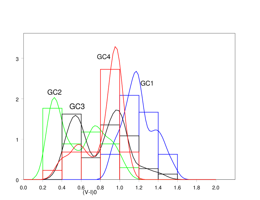
Figure 7: Histograms with density lines of $(V-I)_{0}$ color for the groups of globular clusters found as a result of CA in the LV. Blue solid curve is for GC1, green solid curve is for GC2, black solid curve is for GC3 and red solid curve is for GC4 respectively.

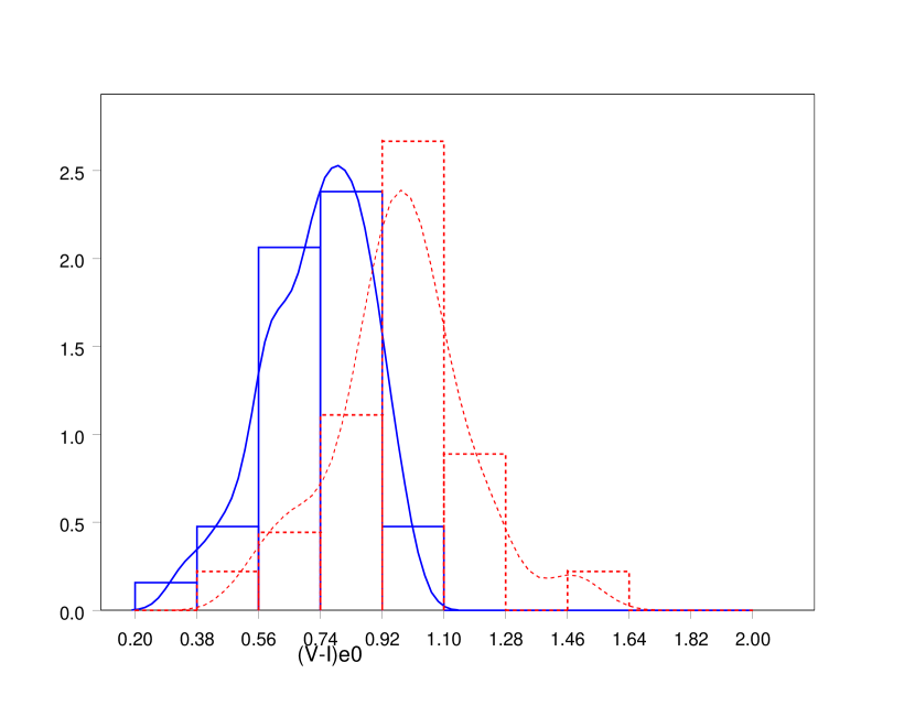
Figure 8: Histograms with density lines of $(V-I)_{e0}$ color for the groups of dwarf galaxies found as a result of CA in the LV. Blue solid line is for G1 galaxies and red dashed line is that for G2.

We have computed the correlations of some of these parameters with the tidal index ($\Theta$) for these dwarf galaxies. The correlations show very high values for G2 galaxies ($r\sim 0.9/0.8,p<0.05$, Table 4) contrary to highly insignificant ones ($r\sim 0.09/0.1,p>>0.05$) for G1 galaxies. This fact indicates that self enrichment supported by stellar and supernovae feed back plays a very important role in the formation of stellar populations in G1 galaxies but star formation is highly regulated by environment as is evident from high tidal indices, low values of correlations of $\Theta$ with scaling parameters, low luminosity - metallicity correlation (Fig. 3) and insignificant rotation of HI mass for G2 galaxies etc. This might be the result of globular clusters formation due to higher velocity collisions in deep potential well leading to more efficient globular cluster formation. In this respect Kumai et al. (1993) have suggested that galaxies in deeper environment (i.e. higher $\Theta$) are more likely to undergo interactions which can increase the random motion of gas clouds within such galaxies. This leads to increase in $S_{N}(orS_{L},S_{M},\hat{T_{b}},log(\eta_{L}),log(\eta_{m})$ etc) with environment. At the same time color histograms (Fig. 5) of GCs as well as of the dwarf galaxies in G2 show major star formation episode (largest peak) at $<(V-I)_{0}>\sim 1.0/0.9$ for GC4 and GC1 GCs and $<(V-I)_{e0}\sim 0.9750;$ (viz. Table 4) for G2 galaxies which corresponds to older burst of star formation (viz. Table 3 $\sim Gyr$; Sharina et al. 2008; Puzia & Sharina 2008). The above phenomenon can be interpreted as star formation has been ceased subsequently due to gas stripping or ram pressure sweeping and evaporation which may give rise to different amount of mass loss as a consequence of the action of the dense environment. Low HI masses as well as low rotation velocities of HI masses for G2 galaxies also support the above scenario. This is in contrast to the low density environment of G1 galaxies which are free of suffering any external triggering. Hence in low density environment younger burst of star formation is possible (Vilchez 1997). This is also clear from the color profiles of GC2 and GC3 GCs (Fig.7) and G1 (Fig. 8) galaxies respectively which have also peaks at $(V-I)\sim 0.3/0.5$ and those correspond to age less than Gyr (Sharina et al. 2005).

When globular clusters evolve their core radii decrease and tidal radii increase. So the quantity $log(r_{t}/r_{c})$ increases. When $log(r_{t}/r_{c})>$2.5 (Chattopadhyay et al. 2009)the globular clusters undergo core collapse i.e. they are dynamically much evolved. Now the values of the above quantity for the four groups of GCs GC1, GC2, GC3 and GC4 found as a result of CA are 1.0115, 1.0735, 1.0721 and 1.2483 respectively. So, GCs of GC4 are dynamically much evolved compared to those in GC1, GC2 and GC3 respectively. As we know most evolved GCs are roundest so with respect to ellipticities GCs of GC4 are more evolved than those in the remaining ones. So accumulating the above fact and values of the peaks of the colors in these four groups we can conclude that GCs of GC4 and GC1 are more evolved than those in GC2 and GC3.

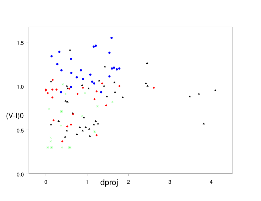
Figure 9: Color ($(V-I)_{0}$) vs projected distances ($d_{proj}$) of the four groups of GCs GC1, GC2, GC3 and GC4. Blue solid circles are for GC1, green stars are for GC2, black triangles are for GC3 and red diamonds are for GC4.

The mean values of $(V-I)_{0}$ for GC1 and GC4 are similar to mean value of that in G2 whereas the mean values of GC2 and GC3 are similar to that in G1 (Tables 4 and 5). So G1 galaxies can be considered as normal sites for the formation of GCs in GC2 and GC3 which are dynamically less evolved (viz. $<Age>\sim$ 5 Gyr for GC4, Table 5). On the other hand G2 galaxies can be considered as places for the formation of of GCs in GC1 and GC4 which are dynamically much evolved hence older (age $\sim$ 7.2 Gyr for GC3, Table 5). Though ellipticities and $log(r_{t}/r_{c})$ for GC1 do not support the above fact but the higher mean value of color $(V-I)_{0}$ indicates that it contains redder GCs which is an indication of older ages. The GCs in GC1 and GC4 are formed by mechanism other than self enrichment (viz. $r(V0,(V-I)_{0})\sim-0.199,p=0.350$ for GC1 and $r(V0,(V-I)_{0})\sim-0.155,p=0.49$ for GC4). From the histograms of colors (Fig. 7) and color vs projected distance (Fig. 9) of the groups GC1, GC2, GC3 and GC4 it is clear that the highest peaks of GCs of GC1 and GC4 occur at higher values of $(V-I)_{0}$. But for GCs in GC2 and GC3 the heights of the peaks at the modes are not very different from one another and they occur even at much lower values of $(V-I)_{0}$ (viz. 0.3/0.5, Table 5). If the correlations between color and projected distance are calculated for the four groups GC1, GC2, GC3 and GC4 these are (0.102, p = 0.635), (0.402, p = 0.109), (0.234, p = 0.164) and (0.091, p= 687) respectively. So it is clear that for GCs of GC2 and GC3 the correlations are moderate at 10 % level of significance .

The correlations between magnitude and projected distance of the above four groups are (0.015, p = 0.945), (0.560, p = 0.019), (0.373, p = 0.023) and ( -0.180, p = 0.422) respectively. This is an indication that the star formation history can be considered to be similar for groups GC1 and GC4 compared to that for GC2 and GC3. Since the GCs in GC1 and GC4 are much evolved than those in GC2 and GC3, and the tidal indices are higher for those in G2 which are their places for formation, it is very likely to assume that the GCs in the outer parts of GC1 and GC4 are tidally stripped from their host galaxies. This does not hold for GCs in GC2 if their host galaxies (considered G1) possess high degree of rotation which is the case as discussed before regarding the rotation of their total HI masses though this is not true for GCs of GC3

6 Summary and conclusions

In the present work statistical approach for classification of LSB dwarf galaxies and globular clusters has been developed. For the classification two statistical techniques are used viz. Principal Component Analysis (PCA) followed by K-means Cluster Analysis (CA) together with the criterion for finding optimum number of homogeneous groups. Through PCA the optimum set of parameters giving maximum variation among the objects is found while the required homogeneous groups are found using CA. The optimum number of groups is found following Sugar & James (2003). For the sample of dwarf galaxies two groups are found primarily indicative of their masses ($M_{V0}$), tidal indices ($\Theta$)and surface brightness averaged over effective radius ($SBV_{e0}$) but irrespective of their morphological indices.

G1 galaxies are massive ($M_{V0}<-13$) with larger amount of HI mass having higher degree of rotation ($V_{m}$) and lower mean value of tidal index with absence of any correlation ($r\sim 0.09/0.1,p>>0.05$; viz Table 4) with scaling parameters. Also there exists moderate mass metallicity correlations among the dwarf galaxies of G1. All these facts indicate that dwarf galaxies of G1 are formed by self enrichment supported by stellar and supernovae feedback. On the other hand G2 galaxies are less massive, have insignificant amount of HI mass with little or absence of any rotation , devoid of any mass metallicity correlation, high values of tidal indices with significant correlations ($r\sim 0.9/0.8,p<0.05$; viz. Table 4) with the scaling parameters. The above mentioned characteristics suggest that environment plays a very important role in formation in the star formation scenario of these dwarf galaxies.

Subsequently a classification of GCs in the LV has been carried out and four groups emerged as a result of such classification. A comparison of the color profiles of the GCs in these groups with those of dwarf galaxies suggest that among the four groups GC1 and GC4 which are dynamically much evolved can be formed in G2 whereas dynamically less evolved GCs in GC2 and GC3 having no significant self-enrichment can be formed in galaxies like G1. Also colors of GCs in GC1 and GC4 bear no correlations with their projected distances while moderate correlation exists for the GCs of GC2 and GC3. This is also true for magnitude vs projected distance correlations. So the star formation history for the GCs of GC1 and GC4 might be speculated to be different from those in GC2 and GC3.

7 Acknowledgements

One of the the authors (Tanuka Chattopadhyay)wishes to thank Department of Science and Technology (DST),India for awarding her a major research project for the work. The authors are grateful to Prof A.K. Chattopadhyay and Emmanuel Davoust for their useful suggestions and help. The authors are also thankful for the suggestions of the referee.

Figure 1: The distortion and jump curves for the classification of dwarf galaxies in the LV

Figure 2: The distortion and jump curves for the classification of globular clusters in the LV

Figure 3: Absolute luminosity in the V-band($M_{V0}$) vs. metallicity ($[Fe/H]$) diagram for the two groups G1 and G2 of dwarf galaxies found as a result of CA in the LV. The black circles (dIrrs) and one black diamond (dIrr/dSph) are for group G1 and green symbols are for G2. dSphs, dIrrs, and dIrrs/dSphs are shown as dots, circles, and asterisks, correspondingly. The best fitted line is for G1 galaxies removing top 2 black circles as outliers. The green line is from S08.

Figure 4: Tidal index ($\Theta$) vs logarithm of scale length in kpc for the two groups G1 and G2 of dwarf galaxies found as a result of CA in the LV. Symbols are the same as in Fig.3. Regression line for G2 was counted removing E443-09 and KKH5 as outliers.

Figure 5: Absolute magnitude in the V-band, corrected for Galactic extinction vs. projected distance of a GC from a center of a galaxy for the two groups G1 and G2 of dwarf galaxies found as a result of CA in the LV. Symbols are the same as in Fig.3. Dotted line is a line of equal central surface brightness for spiral galaxies from S08.

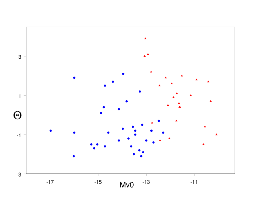
Figure 6: Tidal index ($\Theta$) vs Mass($M_{V0}$) diagram for the two groups G1 and G2 of dwarf galaxies found as a result of CA in the LV. The blue solid circles are for group G1 and red solid triangles are for G2

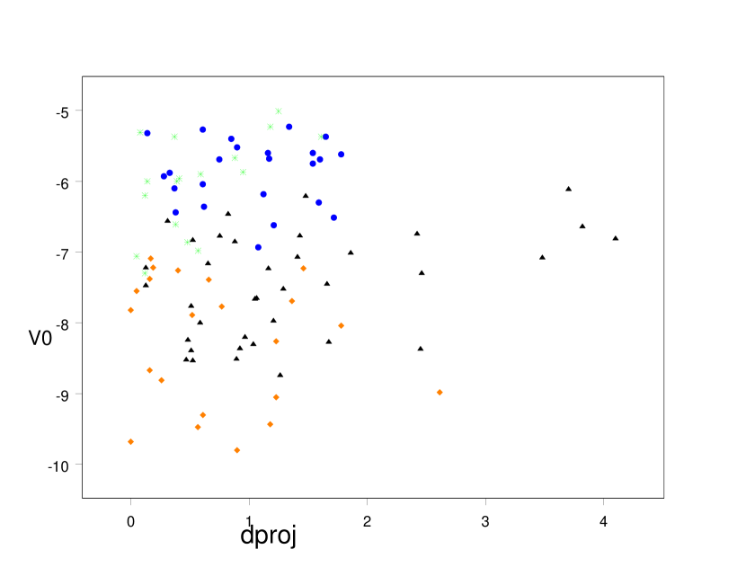
Figure 10: Absolute magnitude V0 vs $d_{proj}$ for the groups of GCs GC1, GC2, GC3 and GC4. The symbols and colors are same as Fig. 9.

Table 1: List of dwarfs in Data Set 1

Name	RA(2000)	DEC(2000)
E349-031	00  08  13.3	-34  34  42.0
E410-005	00  15  31.4	-32  10  48.0
E294-01	00  26  33.3	-41  51  20.0
KDG2	00  49  21.1	-18  04  28.0
E540-032	00  50  24.3	-19  54  24.0
UGC685	01  07  22.3	16  41  02.0
KKH5	01  07  32.5	51  26  25.0
KKH6	01  34  51.6	52  05  30.0
KK16	01  55  20.6	27  57  15.0
KK17	02  00  09.9	28  49  57.0
KKH34	05  59  41.2	73  25  39.0
E121-20	06  15  54.5	-57  43  35.0
E489-56	06  26  17.0	-26  15  56.0
KKH37	06  47  45.8	80  07  26.0
UGC3755	07  13  51.8	10  31  19.0
E059-01	07  31  19.3	-68  11  10.0
KK65	07  42  31.2	16  33  40.0
UGC4115	07  57  01.8	14  23  27.0
DDO52	08  28  28.5	41  51  24.0
D564-08	09  02  54.0	20  04  31.0
D565-06	09  19  29.4	21  36  12.0
KDG61	09  57  02.7	68  35  30.0
KKH57	10  00  16.0	63  11  06.0
HS117	10  21  25.2	71  06  58.0
UGC6541	11  33  29.1	49  14  17.0
NGC3741	11  36  06.4	45  17  07.0
E320-14	11  37  53.4	-39  13  14.0
KK109	11  47  11.2	43  40  19.0
E379-07	11  54  43.0	-33  33  29.0
NGC4163	12  12  08.9	36  10  10.0
UGC7242	12  14  07.4	66  05  32.0
DDO113	12  14  57.9	36  13  08.0
DDO125	12  27  41.8	43  29  38.0
UGC7605	12  28  39.0	35  43  05.0
E381-018	12  44  42.7	-35  58  00.0
E443-09	12  54  53.6	-28  20  27.0
KK182	13  05  02.9	-40  04  58.0
UGC8215	13  08  03.6	46  49  41.0
E269-58	13  10  32.9	-46  59  27.0
KK189	13  12  45.0	-41  49  55.0
E269-66	13  13  09.2	-44  53  24.0
KK196	13  21  47.1	-45  03  48.0
KK197	13  22  01.8	-42  32  08.0
KKs55	13  22  12.4	-42  43  51.0
14247	13  26  44.4	-30  21  45.0
UGC8508	13  30  44.4	54  54  36.0
E444-78	13  36  30.8	-29  14  11.0
UGC8638	13  39  19.4	24  46  33.0
KKs57	13  41  38.1	-42  34  55.0
KK211	13  42  05.6	-45  12  18.0
KK213	13  43  35.8	-43  46  09.0
KK217	13  46  17.2	-45  41  05.0
CenN	13  48  09.2	-47  33  54.0
KKH86	13  54  33.6	04  14  35.0
UGC8833	13  54  48.7	35  50  15.0
E384-016	13  57  01.6	-35  20  02.0
KK230	14  07  10.7	35  03  37.0
DDO190	14  24  43.5	44  31  33.0
E223-09	15  01  08.5	-48  17  33.0
IC4662	17  47  06.3	-64  38  25.0

Table 2: Discriminant analysis for dwarf galaxies in LV. G1, G2 are the groups found by K-means and $G1^{*}$ and $G2^{*}$ are the groups to which dwarfs are assigned by the Discrminant Analysis. N = 60, $N_{correct}$ = 59, Proportion correct = 0.983

		Number of members
DA Clusters	G1	G2
$G1^{*}$	35	1
$G2^{*}$	0	24
Total	35	25

Table 3: Discriminant analysis for GCs in the the LV dwarf galaxies. GC1, GC2, GC3 and GC4 are the groups found by K-means and $GC1^{*}$, $GC2^{*}$, $GC3^{*}$ and $GC4^{*}$ are the groups to which GCs are assigned by the Discrminant Analysis. N = 100, $N_{correct}$ = 97, Proportion correct = 0.97

			No.
DA Clusters	GC1	GC2	GC3	GC4
$GC1^{*}$	23	0	0	0
$GC2^{*}$	0	17	0	1
$GC3^{*}$	1	0	37	1
$GC4^{*}$	0	0	0	20
Total	24	17	37	22

Table 4: Mean values and correlations of the significant parameters for the two groups of dwarfs in the LV

Parameters	G1	G2
Number	35	25
$\Theta$	-0.631 $\pm$0.200	0.880 $\pm$0.287
$[Fe/H]$	-1.8394 $\pm$0.0658	-1.6675 $\pm$ 0.0586
$M_{V0}$	-14.060 $\pm$0.190	-11.742 $\pm$ 0.177
$SBV_{e0}$	22.730 $\pm$ 0.150	24.102 $\pm$ 0.128
$(V-I)_{e0}$	0.7298 $\pm$ 0.0257	0.9750 $\pm$ 0.0391
$logR_{e}$	-0.2827 $\pm$ 0.0331	-0.3842 $\pm$ 0.0357
$V_{m}$	26.12 $\pm$ 3.23	11.11 $\pm$ 3.69
$M_{HI}$	6.571 $\pm$ 2.40	0.516 $\pm$ 0.249
$M_{*V}$	6.69 $\pm$ 3.06	0.41$\pm$ 0.155
$\hat{T_{b}}$	52.6 $\pm$ 15.7	238.1 $\pm$ 96.4
$log(\eta_{L})$	-4.264 $\pm$ 0.224	-4.568 $\pm$ 0.329
$log(\eta_{M})$	-4.616 $\pm$ 0.301	-4.912 $\pm$ 0.47
Correlations	r    p	r    p
$(log\eta_{L},\Theta)$	0.096   0.805	0.987    0.002
$(log\eta_{M},\Theta)$	0.345    0.364	0.956    0.011
$(S_{L},\Theta)$	0.102    0.793	0.889    0.044
$(S_{M},\Theta)$	0.200    0.606	0.896   0.040
$(\hat{T_{b}},\Theta)$	0.460    0.213	0.854    0.065
$([Fe/H],M_{v})$	-0.553    0.001	-0.290    0.160
$(M_{V0},(V-I)_{e0})$	-0.224    0.195	-0.155    0.459

Table 5: Mean values of the significant parameters for the three groups of GCs in the LV

Parameters	GC1	GC2	GC3	GC4
Number	24	17	37	22
$V0$	-5.8765 $\pm$ 0.0954	-6.041 $\pm$ 0.170	-7.481 $\pm$0.123	-8.263 $\pm$ 0.194
$\mu_{V0}$	21.075 $\pm$ 0.097	19.903 $\pm$ 0.140	20.443 $\pm$ 0.141	18.127 $\pm$ 159
$log(r_{h})$	0.8863 $\pm$ 0.0235	0.7024 $\pm$ 0.0287	1.0753 $\pm$ 0.0153	0.7820 $\pm$ 0.0321
$log(r_{t})$	1.5556 $\pm$ 0.0578	1.4077 $\pm$ 0.0672	1.7965 $\pm$0.0557	1.6179 $\pm$ 0.0463
$log(r_{c})$	0.5441 $\pm$ 0.0366	0.3342 $\pm$ 0.0403	0.7244 $\pm$ 0.0197	0.3696 $\pm$ 0.0377
$log(r_{t}/r_{c})$	1.0115 $\pm$ 0.0747	1.0735 $\pm$ 0.0873	1.0721 $\pm$ 0.0625	1.2483 $\pm$ 0.0500
e	0.1542 $\pm$ 0.0208	0.1647 $\pm$ 0.0284	0.1081 $\pm$0.0166	0.10$\pm$ 0.01
$(V-I)_{0}$	1.1996 $\pm$ 0.0340	0.5800 $\pm$ 0.0617	0.8035 $\pm$ 0.0430	0.8332$\pm$ 0.0436
$d_{proj}$	1.014 $\pm$ 0.105	0.563 $\pm$ 0.112	1.354 $\pm$ 0.171	0.740 $\pm$ 0.144
$Age(Gyr)$	*	*	5.0$\pm$1.32	7.2 $\pm$ 1.5
$Z/H$	*	*	-1.167 $\pm$ 0.230	-1.3 $\pm$0.307
$(\alpha/H)$	*	*	0.2 $\pm$0.0632	0.18 $\pm$0.0490

References

- Babu et al. (2009) Babu, G.J., Chattopadhyay, T., Chattopadhyay, A.K. & Mondal, S. 2009, ApJ, 700, 1768.
- Carraro et al. (2001) Carraro, G., Chiosi, C. Girardi, L. & Lia, C. 2001, astro-ph/0105026.
- Chattopadhyay & Chattopadhyay (2006) Chattopadhyay, T. & Chattopadhyay, A.K. 2006, AJ, 131, 2452.
- Chattopadhyay & Chattopadhyay (2007) Chattopadhyay,T. & Chattopadhyay,A. K. 2007,A&A,472,131.
- Chattopadhyay et al. (2009) Chattopadhyay, A.K., Chattopadhyay, T., Davoust, E. et al. 2009, ApJ, 705, 1533.
- Da Costa et al., (2009) Da Costa, G. S., Grebel, E. K., Jerjen, H., Rejkuba, M. & Sharina, M. E., 2009, AJ, 137, 4361
- Davidge (1991) Davidge T.J., 2005, AJ, 130, 2087.
- Dekel & Silk (1986) Dekel A. & Silk J., 1986, ApJ, 303, 39.
- Dekel & Birnboim (2006) Dekel, A. & Birnboim, Y. 2006, MNRAS, 344, 1131.
- Fraix-Burnet et al. (2006) Fraix-Burnet, D., Choler, P. & Douzery, E.J.P. 2006, A&A, 455, 845.
- Geisler et al. (2007) Geisler, D., George, W., Verne V.,S. & Dana I,C. 2007, PASP, 119, 939.
- Georgiev et al. (2010) Georgiev, I.Y., Puzia, T.H., Goudfrooij, P. & Hilker, M. 2010, astro-ph/1004.2039v1.
- Grebel et al. (2003) Grebel, Eva K., Gallagher, John S. & Harbeck,D. 2003, AJ 125, 1926
- Grebel (1999) Grebel E.K. 1999 IAU Symp. 192, eds. P. White lock and R. Cannon ASP Conf. Ser., 17.
- Haines et al. (2006) Haines, C.P.,LaBarbera,F., Mercurio, A. et al. 2006, ApJ, 647, 21.
- Harbeck et al. (2001) Harbeck D., Grebel E.K., Holtzman J., Guhathakurta P., Brandner W., Geisler D., Sarajedini A., Dolphin A., Hurley-Keller D., Mateo M., 2001, AJ, 122, 3092.
- Hirashita (2000) Hirashita, H. 2000, PASJ, 52, 107.
- Hubble (1922) Hubble, E.P. 1922, ApJ, 56, 162.
- Hubble (1926) Hubble, E.P. 1926, ApJ, 64, 321.
- Johnson et al. (1997) Johnson R.A., Lawrence A., Terlevich R.& Carter D., 1997, MNRAS, 287, 333.
- Johnson & Wichern (1998) Johnson, R.A. & Wichern, G. 1998, Applied Multivariate Statistical Analysis (4th ed., Upper Saddle River : Prentice Hall).
- Karachentsev et al. (2004) Karachentsev,I.D., Karachentseva, V.E., Huchtmeier, W.K. & Makarov, D.I. 2004, AJ, 127, 2031.
- Karachentsev et al. (1998) Karachentsev I.D., Makarov D.I., 1998, in proceedings of IAU Symp. 186, Kyoto, 109.
- Karachentseva et al. (1985) Karachentseva V.E., Karachentsev I.D.& B orngen F., 1985, A&A Suppl.Ser., 60, 213.
- Kormendy (1989) Kormendy,J. 1985, ApJ, 295, 73.
- Kroupa (2002) Kroupa P., 2002, MNRAS, 330, 707.
- (27) Kumai, Y., Hashi, Y. & Fujimoto, M. 1993, ApJ, 416, 576.
- Lisker et al. (2007) Lisker, T., Grebel, E. K., Binggeli, B., & Glatt, K. 2007, ApJ, 660,1186.
- Little & Rubin (2002) Little, R.J.A. & Rubin, D.B. 2002, Statistical Analysis with Missing Data (2nd ed.,Wiley Series in Probability and Statistics).
- MacQueen (1967) MacQueen,J.1967,Fifth Berkeley Symp.Math.Statist.Prob.,1,281.
- Mar n-Franch & Aparicio (2002) Mar n-Franch, A. & Aparicio, A. 2002, ApJ, 568, 174.
- Milligan (1980) Milligan,G.W. 1980, Psychometrika, 45, 325.
- Murtagh (1987) Murtagh, F., & Heck, A. 1987, Multivariate Data Analysis ( Dordrecht: Reidel).
- Penny & Conselice (2008) Penny, S.J. & Conselice, C.J. 2008, MNRAS, 383, 247.
- Puzia & Sharina (2008) Puzia, T.H. & Sharina, m. E. 2008 ApJ 674 909.
- Sharina et al. (2008) Sharina, M.E., Karachentsev, I.D.,Dolphin, A.E. et al. 2008, MNRAS, 384, 1544.
- Sharina et al. (2005) Sharina, M.E., Puzia, T.H. & Makarov,D.I. 2005, A&A, 442, 85.
- Shaya & Tully (1984) Shaya, E.J. & Tully, R.B. 1984, ApJ, 281, 56.
- Skillman et al. (1989) Skillman E.D., Kennicutt R.C., Hodge P.W., 1989, ApJ 347, 875.
- Smith (1985) Smith, G.H. 1985, PASP, 97, 1058.
- Sugar & James (2003) Sugar,A.S. & James,G.M.2003,JASA,98,750.
- Tully et al., (2006) Tully, R. Brent, Rizzi, L., Dolphin, A. E., Karachentsev, I. D., Karachentseva, V. E., Makarov, D. I., Makarova, L., Sakai, S. & Shaya, E. J., 2006, AJ 132, 729.
- van den Bergh (2008) van den Bergh,S.2008,MNRAS,385,L20.
- van den Bergh (2007) van den Bergh,S.2007,AJ,134,344.
- Vaduvescu & McCall (2008) Vaduvescu, O. & McCall, M.L. 2008, A&A,487, 147.
- Whitmore (1993) Whitmore, B.C. 1984, ApJ, 278, 61.
- White & Rees (1978) White, S.D.M. & Rees, M.J. 1978, MNRAS, 183, 341.
- Woo et al. (2008) Woo, J., Courteau, S. & Dekel, A. 2008, MNRAS, 390, 1453.
- Vilchez (1997) Vilchez, J.M. 1997, RevMexAA, 6, 30.