Current-induced resonance
in a ferromagnet–antiferromagnet junction

Abstract

We calculate the response of a ferromagnet–antiferromagnet junction to a high-frequency magnetic field as a function of the spin-polarized current through the junction. Conditions are choused under which the response is zero in absence of such a current. It is shown that increasing in the current density leads to proportional increase in the resonance frequency and resonant absorption. A principal possibility is indicated of using ferromagnet–antiferromagnet junction as a terahertz radiation detector.

1 Introduction

On a level with “conventional” spintronics studying effects in ferromagnet/ferromagnet junctions, a new direction has emerged which is related with spin-polarized current effect on the antiferromagnetic layer in ferromagnet/antiferromagnet junction [1]–[14], so that a term “antiferromagnetic spintronics” has appeared [1, 8].

Figure 1: Scheme of the ferromagnet (FM)–antiferromagnet (AFM) junction; NM being a nonmagnetic layer. The main vector directions are shown.

The interest in studying magnetic junctions with antiferromagnetic layers is related with the following features of antiferromagnets. First, this is low, compared to ferromagnets, magnetization in magnetic fields much lower than the exchange field. This allows to neglect demagnetization effect and, that is more significant, leads to substantially lower values of magnetic fields and currents at which switching effects occur. In contrast with ferromagnets, where spontaneous magnetization exists even in absence of magnetic fields and currents, so that the role of the latter consists in changing the magnetization direction, in the antiferromagnets with mutually compensated magnetic sublattices existence of the resulting magnetic moment is due to magnetic fields and/or currents. Second, the eigenfrequency of the magnetic oscillation in antiferromagnets exceeds the similar frequency in ferromagnets by several orders of magnitude, so that the range of possible using of antiferromagnetic structures extends up to terahertz (THz) frequencies.

One of the directions in spintronics is studying the spin-polarized current effect on ferromagnetic resonance in magnetic junctions [15]–[24]. The current effect on the spectrum and damping of the magnetization oscillation in antiferromagnets was studied in Refs. [13, 14]. It was shown that the spin-polarized current effect leads to decrease in damping and to instability of the antiparallel configuration with switching to parallel one. A possibility was noted of creating canted antiferromagnet configuration with appearance of net magnetization under spin-polarized electron injection without external magnetic field.

In present article, we consider forced oscillation of the antiferromagnet magnetization under high-frequency magnetic field in presence of spin-polarized current. The conditions are choused under which the response to the high-frequency is zero when such a current is absent. Under such conditions, the current exerts a strong effect on the antiferromagnet resonant characteristics. Such a current-driven resonator may be used, in principle, as a THz detector.

2 The model and basic equations

Let us consider a magnetic junction consisting of a pinned ferromagnetic (FM) layer, a free antiferromagnetic (AFM) layer, and nonmagnetic (NM) layer closing the electric circuit (Fig. 1). A thin spacer is supposed between FM and AFM layers to prevent exchange interaction through the interface. The current flows perpendicular to the layers (along $x$ axis) in the direction corresponding to electron flux from ferromagnet to antiferromagnet. The easy axis of the antiferromagnet lies in the layer plane (along $y$ axis), the ferromagnet magnetization vector $\mathbf{M}_{F}$ is parallel to $z$ axis.

The AFM layer thickness $L_{AFM}$ is assumed to be small compared to the spin diffusion length, so that the macrospin approximation is valid. In this approximation, the layer magnetization is supposed to be uniform in thickness, while the spin current through the interface is taking into account by means of additional terms in the equations (see Refs. [25, 13] for details). A simplest AFM model is considered with two collinear equivalent sublattices with equal magnetizations, $|\mathbf{M}_{1}|=|\mathbf{M}_{2}|=M_{0}$.

The Landau–Lifshitz–Gilbert equations for the AFM layer in the presence of spin-polarized current and high frequency magnetic field take the following form (see detailed derivation in Ref. [13]):

$$\frac{d\mathbf{M}}{dt}-\frac{1}{2}\frac{\kappa}{M_{0}}\left\{\left[\mathbf{M}\times\frac{d\mathbf{M}}{dt}\right]+\left[\mathbf{L}\times\frac{d\mathbf{L}}{dt}\right]\right\}+\gamma\left[\mathbf{M}\times\mathbf{H}(t)\right]$$

$$+\frac{1}{2}\gamma(\beta+\beta^{\prime})(\mathbf{M}\cdot\mathbf{n})[\mathbf{M}\times\mathbf{n}]+\frac{1}{2}\gamma(\beta-\beta^{\prime})(\mathbf{L}\cdot\mathbf{n})[\mathbf{L}\times\mathbf{n}]$$

$$+K\left[\mathbf{M}\times\left[\mathbf{M}\times\hat{\mathbf{M}}_{F}\right]\right]+P\left[\mathbf{M}\times\hat{\mathbf{M}}_{F}\right]=0,$$ (1)

$$\frac{d\mathbf{L}}{dt}-\frac{1}{2}\frac{\kappa}{M_{0}}\left\{\left[\mathbf{L}\times\frac{d\mathbf{M}}{dt}\right]+\left[\mathbf{M}\times\frac{d\mathbf{L}}{dt}\right]\right\}$$

$$+\gamma\left[\mathbf{L}\times\mathbf{H}(t)\right]-\gamma\Lambda\left[\mathbf{L}\times\mathbf{M}\right]$$

$$+\frac{1}{2}\gamma(\beta+\beta^{\prime})(\mathbf{M}\cdot\mathbf{n})[\mathbf{L}\times\mathbf{n}]+\frac{1}{2}\gamma(\beta-\beta^{\prime})(\mathbf{L}\cdot\mathbf{n})[\mathbf{M}\times\mathbf{n}]$$

$$+K\left[\mathbf{L}\times\left[\mathbf{M}\times\hat{\mathbf{M}}_{F}\right]\right]+P\left[\mathbf{L}\times\hat{\mathbf{M}}_{F}\right]=0.$$ (2)

Here, $\mathbf{M}=\mathbf{M}_{1}+\mathbf{M}_{2}$ is the AFM magnetization vector, $\mathbf{L}=\mathbf{M}_{1}-\mathbf{M}_{2}$ is the antiferromagnetism vector, $\hat{\mathbf{M}}_{F}$ is the unit vector along the FM layer magnetization, $\mathbf{n}$ is the unit vector along the anisotropy axis, $\mathbf{H}(t)$ is the external magnetic field, $\kappa$ is the damping coefficient, $\Lambda$ is the uniform exchange constant, $\beta,\,\beta^{\prime}$ are the intrasublattice and intersublattice anisotropy constants, respectively ($\beta>\beta^{\prime}$ is assumed), $\gamma$ is the gyromagnetic ratio,

$$K=\frac{\mu_{B}Q}{eL_{AFM}M^{2}}j,$$ (3)

$$P=\frac{\gamma\alpha_{sd}\mu_{B}\tau Q}{eL_{AFM}}j,$$ (4)

$j$ is the current density, $\mu_{B}$ is the Bohr magneton, $\alpha_{sd}$ is the (dimensionless) sd exchange interaction constant, $\tau$ is the spin relaxation time in the AFM layer, $Q$ is the FM conductivity spin polarization, $e$ is the electron charge.

The last two terms in the right-hand sides of Eqs. (2) and (2) describe (in the macrospin approximation) the spin-polarized current effect on the antiferromagnet magnetic configuration. There are two mechanisms of this effect. One of them [26, 27] is due to relaxation of the noncollinear (with respect to the AFM magnetization) component of the electron spins with transfer corresponding torque to the lattice. This occurs within a distance comparable with the Fermi wavelength from the FM–AFM interface. The injected spins collinear to AFM magnetization with lost transverse component remain in nonequilibrium state within much longer distance of the order of the spin diffusion length. Such a state is energetically unfavorable. This can lead to change of the lattice magnetic configuration with transition to more favorable state. This is the second mechanism of the spin-polarized electron interaction with magnetic lattice [28, 29]. These mechanisms are described by the terms with $K$ and $P$ coefficients, respectively. It is seen from Eqs. (2) and (2) that the second mechanism is equivalent to the presence of an additional magnetic field $P\hat{\mathbf{M}}_{F}/\gamma$ parallel to the FM magnetization vector. The latter circumstance leads to appearance of a current-induced AFM canted state in absence of external magnetic field.

In the configuration described, $\hat{\mathbf{M}}_{F}=\{0,\,0,\,1\},\;\mathbf{n}=\{0,\,1,\,0\}$. It is suggested that external dc magnetic field is absent, while a high-frequency magnetic field is parallel to the anisotropy axis, $\mathbf{H}(t)=\{0,\,H_{0}\cos\omega t,\,0\}$ with $H_{0}\ll H_{E}$, where $H_{E}\equiv\Lambda M_{0}$ is the exchange field. Under such conditions, the AFM magnetization is zero in absence of the current ($j=0$). Correspondingly, the magnetic susceptibility component $\chi_{yy}$ responsible for absorption of the high-frequency field with the polarization indicated [30] is zero, too, so that AFM resonance does not occur.

3 Spin-polarized current-driven resonance in antiferromagnet

As it was mentioned, antiferromagnet magnetization appears along the ferromagnet magnetization vector $\hat{\mathbf{M}}_{F}$ under spin-polarized current. Precession of the antiferromagnet magnetization vector makes possible the resonance absorption.

Let us calculate the antiferromagnet magnetization with using Eqs. (2) and (2). The high-frequency field is assumed to be low, is taken into account in scope of the linear approximation, and, hence, does not influence the static magnetization, which is [13]

$$\overline{\mathbf{M}}=\{0,\,0,\,\overline{M}_{z}\},\quad\overline{M}_{z}=\frac{P}{\gamma\left(\Lambda+\frac{1}{2}(\beta-\beta^{\prime})\right)}\approx\frac{P}{\gamma\Lambda}.$$ (5)

The corresponding antiferromagnetism vector is

$$\overline{\mathbf{L}}=\{0,\,\overline{L}_{y},\,0\},\quad\overline{L}_{y}=\sqrt{4M_{0}^{2}-\overline{M}_{z}^{2}}.$$ (6)

To calculate the response to the (low) high-frequency field, we linearize Eqs. (2), (2) in small deviations from $\overline{\mathbf{M}},\,\overline{\mathbf{L}}$. The following set of equations is obtained:

$$\frac{\partial M_{x}}{\partial t}-\frac{1}{2}\frac{\kappa}{M_{0}}\left\{-\overline{M}_{z}\frac{\partial M_{y}}{\partial t}+\overline{L}_{y}\frac{\partial L_{z}}{\partial t}\right\}+PM_{y}$$

$$-\frac{1}{2}\gamma(\beta+\beta^{\prime})\overline{M}_{z}M_{y}-\frac{1}{2}\gamma(\beta-\beta^{\prime})\overline{L}_{y}L_{z}+K\overline{M}_{z}M_{x}$$

$$=\gamma\overline{M}_{z}H(t),$$ (7)

$$\frac{\partial M_{y}}{\partial t}-\frac{1}{2}\frac{\kappa}{M_{0}}\overline{M}_{z}\frac{\partial M_{x}}{\partial t}-PM_{x}+K\overline{M}_{z}M_{y}=0,$$ (8)

$$\frac{\partial\widetilde{M}_{z}}{\partial t}+\frac{1}{2}\frac{\kappa}{M_{0}}\overline{L}_{y}\frac{\partial L_{x}}{\partial t}+\frac{1}{2}\gamma(\beta-\beta^{\prime})\overline{L}_{y}L_{x}=0,$$ (9)

$$\frac{\partial L_{x}}{\partial t}-\frac{1}{2}\frac{\kappa}{M_{0}}\left\{\overline{L}_{y}\frac{\partial\widetilde{M}_{z}}{\partial t}-\overline{M}_{z}\frac{\partial\widetilde{L}_{y}}{\partial t}\right\}$$

$$-\gamma\left\{\Lambda+\frac{1}{2}(\beta-\beta^{\prime})\right\}\overline{L}_{y}\widetilde{M}_{z}=0,$$ (10)

$$\frac{\partial\widetilde{L}_{y}}{\partial t}-\frac{1}{2}\frac{\kappa}{M_{0}}\overline{M}_{z}\frac{\partial L_{x}}{\partial t}-\frac{1}{2}\gamma(\beta-\beta^{\prime})\overline{M}_{z}L_{x}=0,$$ (11)

$$\frac{\partial L_{z}}{\partial t}+\frac{1}{2}\frac{\kappa}{M_{0}}\overline{L}_{y}\frac{\partial M_{x}}{\partial t}+\gamma\left\{\Lambda+\frac{1}{2}(\beta-\beta^{\prime})\right\}\overline{L}_{y}M_{x}+K\overline{M}_{z}L_{z}=0,$$ (12)

where $\widetilde{M}_{z}=M_{z}-\overline{M}_{z},\;\widetilde{L}_{y}=L_{y}-\overline{L}_{y}$.

We seek a solution in the form of forced oscillation with frequency $\omega$ of the external magnetic field. We find

$$M_{x}(\omega)=-\frac{\left(-i\omega+P/\eta\right)PH_{0}}{\Lambda\left(\omega^{2}-\Omega^{2}+2i\nu\omega\right)}\equiv\chi_{xy}(\omega)H_{0},$$ (13)

$$M_{y}(\omega)=-\frac{P^{2}H_{0}}{\Lambda\left(\omega^{2}-\Omega^{2}+2i\nu\omega\right)}\equiv\chi_{yy}(\omega)H_{0},$$ (14)

$$\Omega^{2}=2\gamma^{2}H_{A}H_{E}+P^{2}+\left(\frac{\gamma H_{E}}{\eta}\right)^{2},$$ (15)

$$\nu=\gamma H_{E}\left(\kappa+\frac{1}{\eta}\right),$$ (16)

where $H_{A}=(\beta-\beta^{\prime})M_{0}$ is the anisotropy field, $\eta=\alpha\gamma M_{0}\tau$.

Absorption of the high-frequency field is determined by the imaginary part of the diagonal susceptibility

$$\chi^{\prime\prime}_{\|}\equiv\mathrm{Im}\chi_{yy}(\omega)=\frac{2\nu\omega P^{2}}{\Lambda\left[\left(\omega^{2}-\Omega^{2}\right)^{2}+4\nu^{2}\omega^{2}\right]}.$$ (17)

The maximal absorption corresponds to the resonance frequency

$$\omega_{\mathrm{res}}=\sqrt{\Omega^{2}-2\nu^{2}}.$$ (18)

The Q-factor of the system is

$$Q=\frac{\Omega}{2\nu}.$$ (19)

It follows from Eqs. (15) and (16) that the resonance frequency and Q-factor rise under increase in current.

The power absorbed in a unit volume is [30]

$$W=\frac{1}{2}\omega\chi^{\prime\prime}_{\|}H_{0}^{2},$$ (20)

while the linear absorption coefficient for an electromagnetic wave incident on the layer is

$$\Gamma=\frac{8\pi W}{cH_{0}^{2}}=4\pi q\chi^{\prime\prime}_{\|},$$ (21)

where $c$ is the light velocity, $q=\omega/c$ is the wavenumber of the incident electromagnetic wave.

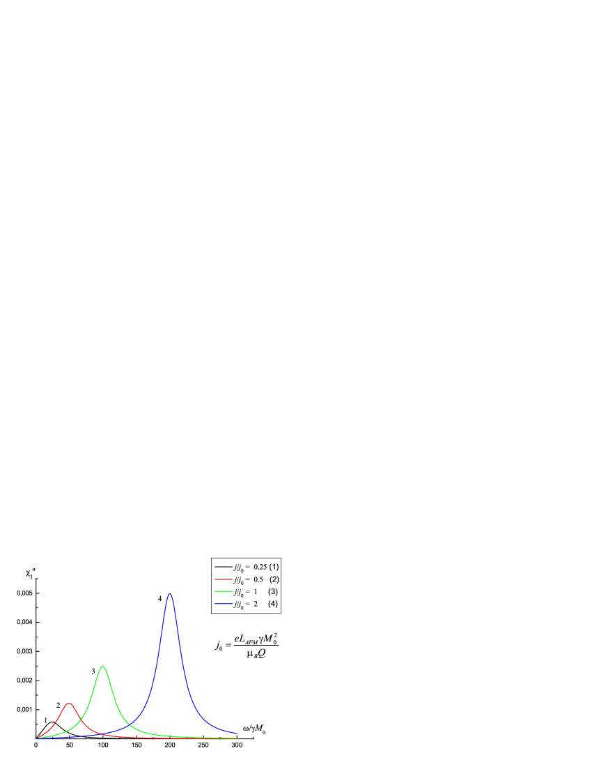
Figure 2: Imaginary part of the diagonal susceptibility $\chi^{\prime\prime}_{\|}$ as a function of the dimensionless frequency $\omega/\gamma M_{0}$ under various (dimensionless) current densities $j/j_{0}$.

4 Discussion

Let us make numerical estimates using the following parameter values: $M_{0}\sim 10^{3}$ G, $\Lambda\sim 10^{3}$, $\alpha\sim 10^{4}$, $\beta\sim\beta^{\prime}\sim 10^{-1}$, $\kappa\sim 10^{-2}$, $\tau\sim 10^{-12}$ s, $L_{AFM}\sim 10^{-6}$ cm. We find $H_{E}\sim 10^{6}$ G, $H_{A}\sim 10^{2}$ G, $\nu\sim 10^{11}$ s^-1, $\Omega\sim 10^{11}$ s^-1, $\eta\sim 10^{2}$. As a scale of the current density, we choose the quantity

$$j_{0}=\frac{eL_{AFM}\gamma M_{0}^{2}}{\mu_{B}Q_{F}},$$ (22)

so that

$$P=\eta\gamma M_{0}\frac{j}{j_{0}}.$$ (23)

With indicated parameter values, $j_{0}\sim 10^{7}$ A/cm². At $j\sim j_{0}$ we have $\Omega\approx P$, i.e., the eigenfrequency is proportional to the current density. The same applies to the resonant absorption.

The absorption spectrum ($\chi^{\prime\prime}_{\|}$ as a function of the dimensionless frequency $\omega/\gamma M_{0}$) with various current densities is shown in Fig. 2. It is seen, that the resonance frequency and resonant absorption rise proportionally to the current density. At $j\sim j_{0}$, we have the resonance frequency about $10^{12}$ c^-1, that corresponds to THz range.

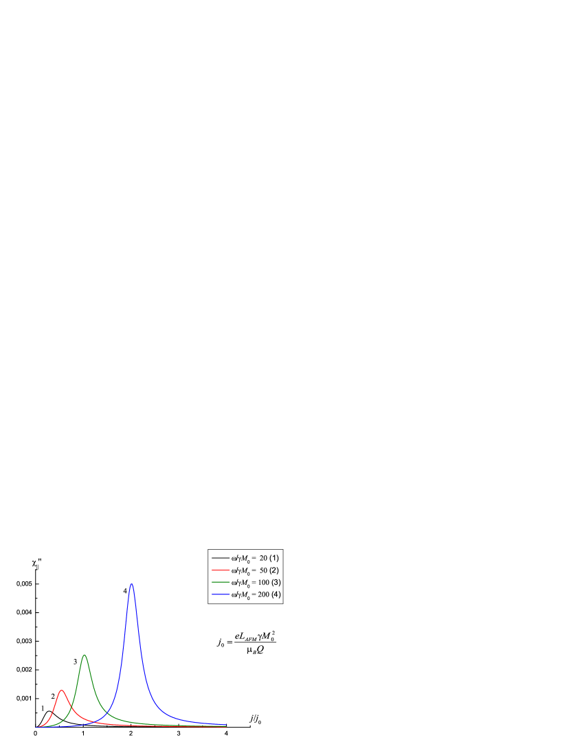
Figure 3: Imaginary part of the diagonal susceptibility $\chi^{\prime\prime}_{\|}$ as a function of the dimensionless current density $j/j_{0}$ at various (dimensionless) frequencies $\omega/\gamma M_{0}$.

The absorption as a function of the current density at various frequencies has the similar form (see Fig. 3 where the same dimensionless variables are used).

At $\Omega=10^{12}$ s${}^{-1},\,\nu=10^{11}$ s^-1 we have $Q=5$. (For comparison: the Q-factor of free oscillation without current

$$Q_{0}=\frac{1}{\kappa}\sqrt{\frac{H_{A}}{2H_{E}}}$$ (24)

is less than 1.) The Q-factor rises under increase in the frequency and/or current density.

For THz radiation ($q\sim 10^{2}$ cm^-1) at $j\sim j_{0}$ the absorption coefficient is $\Gamma\sim 10$ cm^-1, so that the absorption within the thickness of the AFM layer is quite small, $\sim 10^{-5}$–$10^{-4}$. To overcome this difficulty, a multilayer structure of alternating ferromagnet–antiferromagnet layers may be used with electromagnetic wave incident from the butt side (along $z$ axis). The reflection coefficient of the normally incident wave is [31]

$$R=\left|\frac{\widetilde{n}-\widetilde{\mu}}{\widetilde{n}+\widetilde{\mu}}\right|^{2},$$ (25)

where $\widetilde{n}=n+ik$ is the complex index of refraction, $\widetilde{\mu}=\mu^{\prime}+i\mu^{\prime\prime}=1+4\pi(\chi^{\prime}+i\chi^{\prime\prime})$ is the complex magnetic permeability.

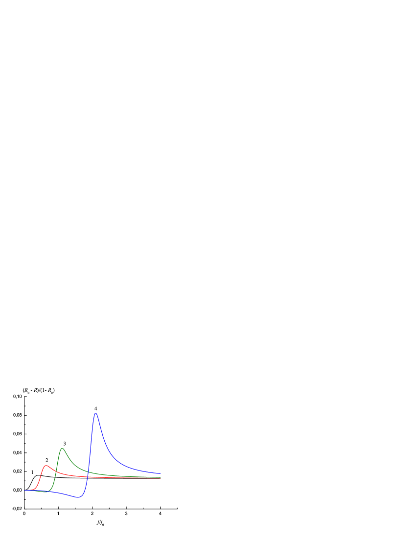
Figure 4: The current-induced relative change of the reflection coefficient as a function of the (dimensionless) current density. The notations are the same as in Fig. 3.

In long wavelength range [31]

$$n\approx k\approx\sqrt{\frac{2\pi\sigma_{0}}{\omega}}\gg 1,\,|\mu|,$$ (26)

where $\sigma_{0}$ is the static conductivity. Therefore, Eq. (25) can written as

$$R=R_{0}-4\pi(1-R_{0})(\chi^{\prime}+\chi^{\prime\prime}),$$ (27)

where $R_{0}$ is the reflection coefficient in absence of the spin-polarized current when $\chi^{\prime}=\chi^{\prime\prime}=0$ under geometry in consideration (see Eq. (14)). The current-induced relative change of the reflection coefficient $(R_{0}-R)/(1-R_{0})=4\pi(\chi^{\prime}+\chi^{\prime\prime})$ as a function of the (dimensionless) current density is shown in Fig. 4. It is seen that $\Delta R=R-R_{0}$ is of the order of $10^{-3}$–$10^{-2}$ at $j\sim j_{0}$ (i. e. $\sim 10^{7}$ A/cm² at chosen parameters). The desired resonance signal can be extracted by the current modulation.

5 Conclusion

The results indicate a possibility of a new effect, namely, current-induced resonance in ferromagnet–antiferromagnet junctions. The resonance frequency and resonant absorption are proportional to the current density through the junction. This opens a principal possibility of using such junctions as current-controlled resonant detectors for THz radiation. Making of corresponding experiments seems to be interesting.

The work was supported by the Russian Foundation for Basic Research, Grant No. 10-02-00030-a.

References

- [1] A.S. Núñez, R.A. Duine, P. Haney, A.H. MacDonald, Phys. Rev. B 73, 214426 (2006).
- [2] Z. Wei, A. Sharma, A.S. Nunez, P.M. Haney, R.A. Duine, J.Bass, A.H. MacDonald, M. Tsoi, Phys. Rev. Lett. 98, 116603 (2007).
- [3] S. Urazhdin, N. Anthony, Phys. Rev. Lett. 99, 046602 (2007).
- [4] P.M. Haney, R.A. Duine, A.S. Núñez, A.H. MacDonald, J. Magn. Magn. Mater. 320, 1300 (2008).
- [5] H. Gomonay, V. Loktev, J. Magn. Soc. Jpn. 32, 535 (2008).
- [6] Z. Wei, A. Sharma, J. Bass, M. Tsoi, J. Appl. Phys. 105, 07D113 (2009).
- [7] H.V. Gomonay, V.M. Loktev, Phys. Rev. B 81, 144127 (2010).
- [8] A.B. Shick, B. Khmelevskyi, O.N. Mryasov, J. Wunderlich, T. Jungwirth, Phys. Rev. B 81, 212409 (2010).
- [9] K.M.D. Hals, Y. Tserkovnyak, A. Brataas, Phys. Rev. Lett. 106, 107206 (2011).
- [10] H.V. Gomonay, R.V. Kunitsyn, V.M. Loktev, arXiv:1106.4231.v2 [cond-mat.mtrl-sci].
- [11] Yu.V. Gulyaev, P.E. Zilberman, E.M. Epshtein, J. Commun. Technol. Electron. 56, 863 (2011).
- [12] J. Linder, Phys. Rev. B 84, 094404 (2011).
- [13] Yu.V. Gulyaev, P.E. Zilberman, E.M. Epshtein, J. Exp. Theor. Phys. 114, 296 (2012).
- [14] Yu.V. Gulyaev, P.E. Zilberman, E.M. Epshtein, J. Commun. Technol. Electron. 57, (2012) (to be published).
- [15] G.D. Fuchs, J.C. Sankey, V.S. Pribiag, L. Qian, P.M. Braganca, A.G.F. Garcia, E.M. Ryan, Zhi-Pan Li, O. Ozatay, D.C. Ralph, R.A. Buhrman, Appl. Phys. Lett. 91, 062507 (2007).
- [16] S. Petit, N. de Mestier, C. Baraduc, C. Thirion, Y. Liu, M. Li, P. Wang, B. Dieny, Phys. Rev. B 78, 184420 (2008).
- [17] O. Posth, N. Reckers, R. Meckenstock, G. Dumpich, J. Lindner, J. Phys. D: Appl. Phys. 42, 035003 (2009).
- [18] C.T. Boone, J.A. Katine, J.R. Childress, V. Tiberkevich, A. Slavin, J. Zhu, X. Cheng, I. N. Krivorotov, Phys. Rev. Lett. 103, 167601 (2009).
- [19] T. Seki, H. Tomita, A.A. Tulapurkar, M. Shiraishi, T. Shinjo, Y. Suzuki, Appl. Phys. Lett. 94, 212505 (2009).
- [20] Y. Guan, J.Z. Sun, X. Jiang, R. Moriya, L. Gao, S.S.P. Parkin, Appl. Phys. Lett. 95, 082506 (2009).
- [21] W. Chen, G. de Loubens, J.-M.L. Beaujour, J.Z. Sun, A.D. Kent, Appl. Phys. Lett. 95, 172513 (2009).
- [22] R.-X. Wang, P.-B. He, Q.-H. Liu, Z.-D. Li, A.-L. Pan, B.-S. Zou, Y.-G. Wang, J. Magn. Magn. Mater. 322, 2264 (2010).
- [23] T. Staudacher, M. Tsoi, Thin Solid Films 519, 8260 (2011).
- [24] Y. Okutomi, K. Miyake, M. Doi, H.N. Fuke, H. Iwasaki, M. Sahashi, J. Appl. Phys. 109, 07C727 (2011).
- [25] Yu.V. Gulyaev, P.E. Zilberman, A.I. Panas, E.M. Epshtein, J. Exp. Theor. Phys. 107, 1027 (2008).
- [26] J.C. Slonczewski, J. Magn. Magn. Mater. 159, L1 (1996).
- [27] L. Berger, Phys. Rev. B 54, 9353 (1996).
- [28] C. Heide, P.E. Zilberman, R.J. Elliott, Phys. Rev. B 63, 064424 (2001).
- [29] Yu.V. Gulyaev, P.E. Zilberman, E.M. Epshtein, R.J. Elliott, JETP Lett. 76, 155 (2002).
- [30] A.I. Akhiezer, V.G. Baryakhtar, S.V. Peletminskii, Spin Waves, North-Holland Publ. Co., Amsterdam, 1968.
- [31] A.V. Sokolov, Optical Properties of Metals, American Elsevier Publ. Co., 1967.