Abstract: Sparsity-promoting priors have become increasingly popular over recent years due to an increased number of regression and classification applications involving a large number of predictors. In time series applications where observations are collected over time, it is often unrealistic to assume that the underlying sparsity pattern is fixed. We propose here an original class of flexible Bayesian linear models for dynamic sparsity modelling. The proposed class of models expands upon the existing Bayesian literature on sparse regression using generalized multivariate hyperbolic distributions. The properties of the models are explored through both analytic results and simulation studies. We demonstrate the model on a financial application where it is shown that it accurately represents the patterns seen in the analysis of stock and derivative data, and is able to detect major events by filtering an artificial portfolio of assets.

Key-words: generalized hyperbolic, Gaussian mixture models, sparsity, dynamic regression

Modèles linéaires bayésiens dynamiques et parcimonieux

Résumé : Les distributions a priori encourageant la parcimonie sont devenues de plus en plus populaires au cours des dernières années du fait du nombre d’applications croissantes en régression et classification impliquant un grand nombre de prédicteurs. Dans le cas où les observations sont recueillies au cours du temps, il est souvent irréaliste de considérer que la structure de parcimonie est fixée au cours du temps. Nous proposons ici une classe originale de modèles bayésiens linéaires flexibles pour la modélisation dynamique parcimonieuse. La classe de modèles proposée repose sur l’utilisation de distributions hyperboliques généralisées. Les propriétés de ces modèles sont explorées au travers de résultats analytiques et de simulations. Enfin, nous présentons une application de ce modèle en finance.

Mots-clés : Modèles parcimonieux, distribution hyperbolique généralisée, modèle de mélange de gaussiennes, régression linéaire dynamique

1 Introduction

Over recent years, there has been an increased number of regression and classification applications involving high-dimensional data. In these scenarios, it is common to have a large number of predictors, a number of them being irrelevant. The need to appropriately restricts the number of predictors for improved statistical efficiency and predictive abilities has generated a large body of work. In the non-Bayesian literature sparse regression analysis via penalised likelihood has become extremely popular since the seminal lasso paper (Tibshirani,, 1996); in the Bayesian literature, spike-and-slab priors have historically been favoured (Mitchell and Beauchamp,, 1988; Zhang et al.,, 2007). Unfortunately, spike and slab priors are notoriously difficult to fit, leading to a renewed interest in proposing alternative sparsity-promoting prior models.

It is well-known that the Lasso estimate for linear regression parameters can be interpreted as the MAP (Maximum A Posteriori) estimate when the regression parameters are assigned independent Laplace priors. From a Bayesian perspective, the use of MAP estimators lacks solid justification; however, although they are not sparse in the exact sense, Bayesian posterior medians are remarkably similar in value to lasso estimates (Park and Casella,, 2008) and provide credible intervals which can help in guiding variable selection. Additionally it has been observed empirically that Markov chain Monte Carlo (MCMC) mix quite well for such models (Kyung et al.,, 2010). However, it is well-known that the lasso estimates and its Bayesian version suffer from various problems. In particular, coefficients can get shrunk towards zero even when there is overwhelming evidence in the likelihood that they are non-zero. There has been much work in the non-Bayesian and Bayesian literature to improve over this; for example, a number of sparsity-promoting non-concave log prior distributions have been proposed which reduce bias in the estimates of large coefficients. Recent work includes (Griffin and Brown,, 2007; Caron and Doucet,, 2008; Lee et al.,, 2010; Griffin and Brown,, 2010) and Bayesian interpretations of the group lasso and elastic net estimators (Bornn et al.,, 2010; Li and Lin,, 2010; Kyung et al.,, 2010). Although the above priors result in non-sparse posterior median and mean estimates, many arguments have been advocated in favour of their use, see e.g. (Kyung et al.,, 2010).

In the context of time series, it is of particular interest to allow for the sparsity pattern to evolve over time as a predictor which is highly relevant in a given time period may become irrelevant later on. Dynamic sparsity modelling is an important topic that has received much less attention in the literature. From a non-Bayesian perspective, several authors have proposed to adapt the elastic net, fused lasso or group lasso to accommodate dynamic models (Angelosante et al.,, 2009; Angelosante and Giannakis,, 2009; Vaswani,, 2008; Jacob et al.,, 2009). From a Bayesian perspective, dynamic spike-and-slab type models have been recently proposed: Nakajima and West, (2011) associate to each predictor a latent process and this predictor is only included in the regression when the magnitude of its associated latent process is above a given latent threshold, whereas Ziniel et al., (2010) associate to each predictor a latent binary inclusion/exclusion Markov chain. We follow here an alternative approach based on the construction of dynamic sparsity-promoting priors. Similar constructions were also recently proposed independently in (Sejdinović et al.,, 2010) and (Kalli and Griffin,, 2012). However, the model presented here is much more flexible. It relies on a scale mixture of normal distributions where the mixing distribution is itself a generalized inverse Gaussian resulting in a multivariate generalized hyperbolic distribution. This scale mixture of normals representation can be used to derive tailored Markov chain Monte Carlo (MCMC) and Sequential Monte Carlo (SMC) methods for inference.

The rest of the paper is organized as follows. In Section 2, we review the generalized hyperbolic distribution and show that it includes numerous sparsity-promoting priors used in the literature. Section 3 presents our dynamic sparsity model and establishes some of its properties. Section 4 proposes several Bayesian computational procedures to perform inference. We demonstrate the model on simulated data and an application to financial data in Sections 5 and 6.

2 Sparse Bayesian regression

2.1 Bayesian regression model

Consider the following standard regression model where

$$y=X\beta+\epsilon$$ (1)

where $y$ is the $n\times 1$ vector of responses, $\beta=\left(\beta_{1},...,\beta_{p}\right)^{\text{T}}$ the vector of regression parameters, $X$ is the $n\times p$ design matrix, and $\epsilon$ is the $n\times 1$ vector of independent and identically distributed normal errors with mean $0$ and variance $\sigma^{2}$. In a Bayesian approach, we adopt a prior density $\pi\left(\beta\right)=\prod_{j=1}^{p}\pi\left(\beta_{j}\right)$. Park and Casella, (2008) proposed to use independent Laplace priors, motivated by the fact that lasso estimates could be interpreted as the Bayes posterior mode under this prior (Tibshirani,, 1996). Laplace priors can be expressed as scale mixture of normal distributions (Andrews and Mallows,, 1974; West,, 1987), hence admit a hierarchical construction. Other models, based on scale mixture of normals, have been proposed in the literature (Tipping,, 2001; Caron and Doucet,, 2008; Griffin and Brown,, 2010). Several of these distributions can be considered as particular case of the generalized hyperbolic distribution, which we review in the next section.

2.2 Generalized hyperbolic distribution

Let $\beta_{j}\in\mathbb{R}$, and suppose the following Gaussian mixture model

$$\beta_{j}|\tau_{j} \sim\mathcal{N}(\mu,\tau_{j})$$ (2)

$$\tau_{j} \sim GiGauss(\nu,\delta,\gamma)$$ (3)

where $\mathcal{N}(\mu,\sigma^{2})$ denotes the Gaussian distribution of mean $\mu$ and variance $\sigma^{2}$ and $GiGauss(\nu,\delta,\gamma)$ is the generalized inverse Gaussian distribution (Barndorff-Nielsen and Shephard,, 2001) of parameters $\nu,\delta,\gamma$ whose probability density function is

$$\frac{(\gamma/\delta)^{\nu}}{2K_{\nu}(\delta\gamma)}x^{\nu-1}\exp\left(-\frac{1}{2}(\delta^{2}x^{-1}+\gamma^{2}x)\right)\text{, }x>0$$ (4)

$\beta_{j}$ then follows a generalized hyperbolic distribution of pdf

$$\frac{(\gamma/\delta)^{\nu}}{\sqrt{2\pi}\gamma^{\nu-1/2}K_{\nu}(\delta\gamma)}\left(\sqrt{\delta^{2}+(\beta_{j}-\mu)^{2}}\right)^{\nu-1/2}K_{\nu-1/2}\left(\gamma\sqrt{\delta^{2}+(\beta_{j}-\mu)^{2}}\right)$$ (5)

where $K_{a}(z)$ is the modified Bessel function of the third kind. We write $\beta_{j}\sim GH(\mu,\nu,\delta,\gamma)$. When $\mu=0$, the distribution is concentrated around $0$. For some values of the parameters $\nu$, $\delta$ and $\gamma$, the pdf will be concentrated around 0 with heavy tails, which makes it a desirable prior distribution for sparse linear regression. The generalized hyperbolic distribution generalizes several distributions that have been used as sparsity-promoting priors:

1. $\nu=-1/2$: Normal inverse Gaussian law (Caron and Doucet,, 2008)

2. $\delta=0$, $\nu>0$: Normal gamma law (Caron and Doucet,, 2008; Griffin and Brown,, 2010)

3. $\delta=0$, $\nu=1$: Laplace law (Tibshirani,, 1996; Park and Casella,, 2008)

4. $\gamma=0$, $\nu<0$: Student’s law (Tipping,, 2001)

All of these priors have been described as suitable prior distributions for promoting sparsity/shrinkage in Bayesian regression models. In some cases, they have been shown to give better predictive performances than spike-and-slab priors in regression (Griffin and Brown,, 2010). The mixing properties of the associated Markov chain Monte Carlo algorithms are also generally considered to be superior due to the smooth scale mixture representation.

The probability density functions of the generalized hyperbolic distribution for different values of the parameters are represented in Figure 1, where we see that the parameters $\nu$, $\delta$ and $\gamma$ provide significant control over the behavior of the mode and tails.

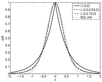
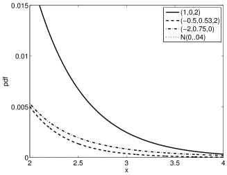
Figure 1: Probability density functions of the generalized hyperbolic distribution for several values of $(\nu,\delta,\gamma)$ correspond to a Laplace, Normal inverse Gaussian and Student t distribution. The pdf of the normal distribution is also shown for comparison. (a) Behavior around 0 and (b) Tail behavior.

3 Dynamic Sparse Bayesian regression

We now consider the problem of successive linear regression models

$$y_{t}=X_{t}\beta_{t}+\varepsilon_{t}$$ (6)

where $t=1,\ldots,T$ is a time index, $\varepsilon_{t}\sim\mathcal{N}(0,\sigma^{2}I_{n})$, $X_{t}$ is a $n\times p$ design matrix, $I_{n}$ is the $n\times n$ identity matrix and $\beta_{t}\in\mathbb{R}^{p}$. Assume a priori independence of the different components $j=1,\ldots,p$

$$\pi(\beta_{1:T})=\prod_{j=1}^{p}\pi(\beta_{j,1:T})$$ (7)

We assume that the true vector $\beta_{t}$ is sparse, and that the sparsity pattern (indices of elements with zero values) is slowly evolving over time. We first consider a simple particular case of group sparsity where the sparsity pattern is unchanged over time, and introduce the multivariate hypergeometric distribution. We then describe how to use this distribution to define models where the sparsity pattern evolves smoothly over time, while highlighting several interesting statistical properties.

3.1 Multivariate generalized hyperbolic

Assume as a simple starting case that we want the sparsity pattern to be shared across time. This can be achieved by considering a hierarchical Gaussian model where the variance is shared over time. Suppose that, for $t=1,\ldots,T$

$$\beta_{j,t}|\tau_{j}\sim\mathcal{N}(\mu,\tau_{j}\Sigma)$$ (8)

where $\mu\in\mathbb{R}^{p}$, $\Sigma$ is a positive semi-definite $p\times p$ matrix, and $\tau_{j}\sim GiGauss(\nu,\delta,\gamma)$. Then $\beta_{j,1:T}\in\mathbb{R}^{T}$ follows the multivariate generalized hyperbolic distribution of pdf

$$\frac{(\gamma/\delta)^{\nu}}{(2\pi)^{p/2}\gamma^{\nu-p/2}K_{\nu}(\delta\gamma)}q^{\nu-p/2}K_{\nu-p/2}(\gamma q)$$ (9)

where $q=\sqrt{\delta^{2}+(\beta_{j,1:T}-\mu)^{T}\Sigma^{-1}(\beta_{j,1:T}-\mu)}$. We write $\beta_{j,1:T}\sim mGH(\mu,\nu,\delta,\gamma,\Sigma)$. Shared sparsity pattern over the $\beta_{j,t}^{\prime}s$ is obtained through the shared variance term $\tau_{j}$. The matrix $\Sigma$ allows one to introduce correlation between variables; again, such priors have been studied in the literature on sparse models. In particular, the group lasso prior (Yuan and Lin,, 2006; Raman et al.,, 2009; Kyung et al.,, 2010) defined by

$$\pi(\beta_{j,1:T})\propto\exp(-\gamma\left\|\beta\right\|_{\Sigma})$$ (10)

is a special case of the multivariate hyperbolic when $\nu=\frac{p+1}{2}$, $\mu$ is the null vector and $\delta=0.$ Other special cases such as the multivariate normal gamma and normal inverse Gaussian have also been studied by Caron and Doucet, (2008).

3.2 Statistical model

We now turn to the use of the multivariate generalized hyperbolic distribution in the modeling of data with dependent and varying sparsity structure. We are interested in defining a model for $\pi(\beta_{j,1:T})$ that introduces correlations in time both

1. in the sparsity pattern: if the vector of regressors is sparse at time $t$, then it is more likely to be sparse at time $t+1$, and

2. in the value of non-zero coefficients.

These properties will be obtained by considering a particular decomposition of the joint distribution $\pi(\beta_{j,1:T})$ with multiple overlapping groups. Consider the following decomposition of the joint distribution:

$$\pi(\beta_{j,1:T})=\frac{\prod_{t=d}^{T}\pi(\beta_{j,t-d:t})}{\prod_{t=d}^{T-1}\pi(\beta_{j,t-d+1:t})}$$ (11)

where $\beta_{j,t-d:t}$ is marginally $mGH(0_{d+1},\nu,\delta,\gamma,\Sigma_{d+1})$, where $d>0$, $0_{d}$ is the null vector of length $d$,

$$\Sigma_{d}=\left(\begin{array}[c]{ccccc}1&\alpha&\ldots&\alpha^{d-1}\\ \alpha&1&\ldots&\ldots\\ \ldots&\ldots&\ldots&\ldots\\ \alpha^{d-1}&\alpha^{d-1}&\ldots&1\end{array}\right)$$

and $\alpha\in[0,1]$. In particular, if $\nu=\frac{d+2}{2}$ and $\delta=0$, then $\beta_{j,t-d:t}$ follows the group lasso distribution (10).

The model can be alternatively defined by the following d-order Markov model ($d>0$)

$$\beta_{j,1:d}\sim mGH(0_{d},\nu,\delta,\gamma,\Sigma_{d})$$ (12)

and for $t>d$

$$\beta_{j,t}|\beta_{j,1:t-1}\sim GH(\alpha\beta_{j,t-1},\nu-d/2,\sqrt{1-\alpha^{2}}\sqrt{\delta^{2}+\left\|\beta_{j,t-d:t-1}\right\|_{\Sigma_{d}}^{2}},\frac{\gamma}{\sqrt{1-\alpha^{2}}})$$ (13)

where $\left\|x\right\|_{\Sigma}=\sqrt{x^{T}\Sigma^{-1}x}$ is the Mahalanobis distance. In the case $d=0$, $\beta_{j,t}$ are iid $GH(0,\nu,\delta,\gamma)$. Using the scale mixture representation of the generalized hyperbolic distribution, the predictive distribution (13) can be equivalently expressed as a scale mixture of normals with latent variables $\tau_{j,t}$

$$\tau_{j,t}|\beta_{j,1:t-1} \sim GiGauss\left(\nu-d/2,\sqrt{\delta^{2}+\left\|\beta_{j,t-d:t-1}\right\|_{\Sigma_{d}}^{2}},\gamma\right)$$

$$\beta_{j,t}|\tau_{j,t},\beta_{j,t-1} \sim\mathcal{N}\left(\alpha\beta_{j,t-1},(1-\alpha^{2})\tau_{j,t}\right).$$

The model has the following statistical properties:

1. The model is first-order stationary with

   $$\beta_{j,t}\sim GH(0,\nu,\delta,\gamma)$$

2. For any $h\leq d$

   $$\beta_{j,t-h:t}\sim mGH(0_{h+1},\nu,\delta,\gamma,\Sigma_{h+1})$$

3. The parameter $0\leq d\leq T-1$ tunes the evolution of the sparsity pattern over time, and we have the following special cases

   • $d=0$, we have independence between the sparsity patterns over time and $\beta_{j,t}$ are iid $GH(0,\nu,\delta,\gamma)$

   • $d=T-1$, the sparsity pattern is shared over time and $\beta_{j,1:T}\sim mGH(0_{T},\nu,\delta,\gamma,\Sigma_{T})$

4. The parameter $\alpha\in[0,1]$ tunes the correlation between regression coefficient values at successive time steps.

These properties make the model very appealing for dynamic linear regression. First, by choosing the parameters $\nu$, $\delta$ and $\gamma$ based on the large literature on sparse Bayesian regression, the user can define the level of sparsity desired in the signal. For example, if $\delta=0$ and $\nu>0$ (normal-gamma case) smaller values of $\nu$ will favor sparser solutions. Second, the user will define how this sparsity pattern is going to evolve over time, from the two extreme cases $d=0$ (independent sparsity pattern over time) and $d=T$ (shared sparsity). Between those two extremes, the value of $d$ will tune how often the time series can alternate between sparse and non-sparse periods. This effect can be seen by looking at the autocorrelation plot for $\beta_{t}^{2}$, as shown in figures 2 and 3. The shared sparsity pattern induces a minimum level of autocorrelation over the lag $d$, as can be seen from Figure 3 for $\alpha=0$. Finally, the parameter $\alpha$ tunes the correlation between non-zero coefficients, in a classical way, and we have $\text{corr}(\beta_{t},\beta_{t-1})=\alpha$.

(a) $d=5$

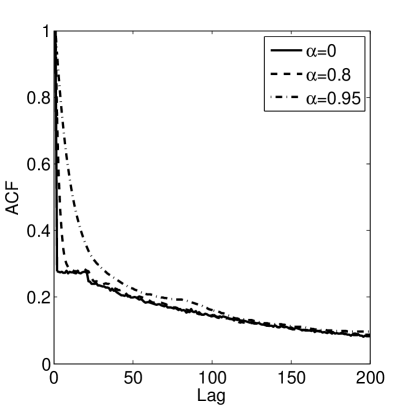
(b) $d=20$

Figure 2: Autocorrelation function for $\beta_{t}^{2}$ from the statistical model defined by Eq. (12) and (13) with $\nu=0.1$, $\delta=0.01$, $\gamma=1$, $T=10^{6}$ and (a) $d=5$, (b) $d=20$. For each value of $d$, three plots are represented with $\alpha=0.00,0.80,0.95$. Note that $d=0$ is not represented, since the variables $\beta_{t}$ are independent in that case. (b) For $d=20$, we can clearly see that the correlation for $\beta_{t}^{2}$ is due to both $\alpha$ and the shared sparsity pattern; after lag 100, the correlation remains due to the shared sparsity pattern. For $\alpha=0$ (black line) we can clearly see a threshold on autocorrelation, which is due to the shared sparsity pattern induced by the model.

Figure 3: Autocorrelation function for $\beta_{t}^{2}$ from the statistical model defined by Eq. (12) and (13) with $\nu=0.1$, $\delta=0.01$, $\gamma=1$, $T=10^{6}$ and $\alpha=0$. Three plots are represented with $d=5,20,100$. As $\alpha=0$, the samples $(\beta_{t})$ are uncorrelated, and the autocorrelation for $\beta_{t}^{2}$ is due to the shared sparsity pattern.

In Figure 4, we represent some samples from this model for different values of $d$ and $\alpha$, to show how the sparsity pattern evolves over time depending on this parameter. This figure motivates the model for use in the modeling of stock volatility. Specifically, stock prices (and trading activity) go through alternating periods of inactivity and alacrity, making the multivariate generalized hyperbolic distribution a suitable modeling choice.

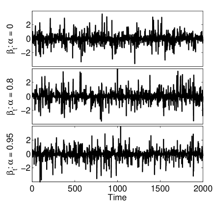
(a) $d=0$

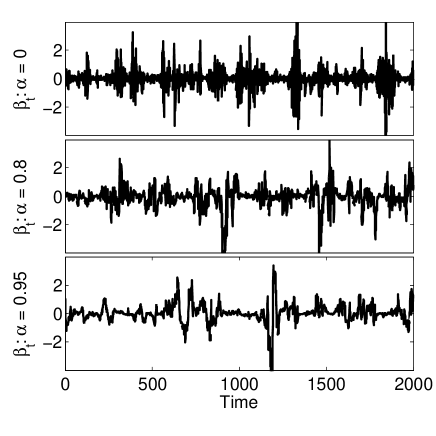
(b) $d=5$

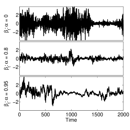
(c) $d=20$

(d) $d=2000$

Figure 4: Samples from the statistical model defined by Eq. (12) and (13) with $\nu=0.1$, $\delta=0.01$, $\gamma=1$, $T=2000$ and (a) $d=0$, (b) $d=5$, (c) $d=20$, (d) $d=T$. For each value of $d$, three draws are represented with $\alpha=0.00,0.80,0.95$. (a) For $d=0$, the variables $\beta_{t}$ are independent and the sparsity pattern is not shared. (b,c) For $d=5,20$, the sparsity pattern can evolve over time, and the process alternates regions close to zero and away from zero. (d) For $d=T$, the sparsity pattern is shared, and the $\beta_{t}$ are either all close to zero (bottom figure in (d)) or away from zero (top and middle figure in (d)).

The model defined by Equations (12) and (13) relies on an integer $d$ that tunes the evolution of the sparsity pattern. One might want to consider this parameter as varying over time, and estimate this value. We could then put a prior on $d_{t}$, e.g. a Markov model

$$d_{t}|d_{t-1}\sim Bin(d_{t-1}+1,\rho)$$

where $\rho\in[0,1]$ and $Bin(n,\rho)$ is the binomial distribution. Alternatively, any distribution with support $\{0,\ldots,d_{t-1}+1\}$ may be used.

4 Algorithms

The full posterior distribution described in the previous section is intractable; we therefore present two algorithms, one which provides fully Bayesian estimates of the regression coefficients, and the other which provides approximate MAP estimates.

4.1 Approximate MAP estimation

MAP estimation requires maximization of the following objective function

$$\sum_{t=1}^{T}\log p(y_{t}|\beta_{t})+\sum_{t=d}^{T}\sum_{j=1}^{p}\log\pi(\beta_{j,t-d:t})-\sum_{t=d}^{T-1}\sum_{j=1}^{p}\log\pi(\beta_{j,t-d+1:t})$$ (14)

This objective function is not convex and does not admit any latent variable construction that might enable the use of an EM algorithm. We propose here an online algorithm to perform approximate MAP estimation. The algorithm will successively maximize $p(\beta_{t}|\widehat{\beta}_{1:t-1},y_{t})$ w.r.t. $\beta_{t}$ for $t=1,\ldots,T$. At each time $t$, we therefore consider optimization of the following objective function w.r.t. $\beta_{t}$

$$\log p(\beta_{t}|\widehat{\beta}_{t-d:t-1})+\log p(y_{t}|\beta_{t}).$$ (15)

It is easy to show that

$$\beta_{j,t}|\beta_{j,t-d:t-1}\sim GH\left(\alpha\beta_{j,t-1},\nu-\frac{d}{2},\sqrt{\delta^{2}+\left\|\beta_{j,t-d:t-1}\right\|_{\Sigma_{d}}^{2}},\frac{\gamma}{\sqrt{1-\alpha^{2}}}\right)$$ (16)

and we can therefore solve (15) with an EM algorithm using the scale mixture of Gaussian representation of the generalized hyperbolic distribution Dempster et al., (1977); Caron and Doucet, (2008).

We now propose a second algorithm to obtain approximate MAP estimates. Consider here that $\nu=(d+2)/2$, $d$ is fixed and known and $\delta=0$. We can solve the following group lasso sliding window optimization problem at time $t>d$, by maximizing according to $\beta_{t-d:t}$

$$\log p(\beta_{t-d:t})+\log p(Y_{t-d:t}|\beta_{t-d:t})$$ (17)

which reduces to minimizing

$$\frac{1}{2\sigma^{2}}\left\|Y_{t-d:t}-X_{t-d:t}\beta_{t-d:t}\right\|^{2}+\gamma\sum_{j=1}^{p}\left\|\beta_{j,t-d:t}\right\|_{\Sigma_{d+1}},$$ (18)

a convex group lasso problem (Yuan and Lin,, 2006) for which efficient algorithms exist.

4.2 Sequential Monte Carlo algorithm

While the previous algorithms conduct approximate MAP inference, we can also write a sequential Monte Carlo (SMC) algorithm to conduct fully Bayesian inference (Doucet et al.,, 2001). Particularly, as memory requirements prevent implementing a particle filter with 1,000,000 particles, we employ the particle independent Metropolis-Hastings algorithm (Andrieu et al.,, 2010) to approximate the full posterior $\pi(\beta_{1:T},d_{1:T}|y_{1:T})$. We can use latent variables to produce efficient proposal distributions for $\beta_{t}$

$$\text{for }j=1,\ldots,p,~{}\ \tau_{j,t}|\beta_{j,t-d_{t}:t-1},d_{t}\sim GiGauss(\nu-d_{t}/2,\sqrt{1-\alpha^{2}}\sqrt{\delta^{2}+\left\|\beta_{j,t-d_{t}:t-1}\right\|_{\Sigma_{d_{t}}}},\frac{\gamma}{\sqrt{1-\alpha^{2}}})$$ (19)

and

$$\beta_{t}|\tau_{t},y_{t}\sim\mathcal{N}(\mu_{t},\Sigma_{t})$$ (20)

with $\mu_{t}=(\sigma_{t}^{2}D_{\tau_{t}}^{-1}+X_{t}^{\prime}X_{t})^{-1}(\alpha\sigma_{t}^{2}D_{\tau_{t}}^{-1}\beta_{t-1}+X_{t}^{\prime}y_{t})$ and $\Sigma_{t}=(D_{\tau_{t}}^{-1}+X_{t}^{\prime}X_{t}/\sigma_{t}^{2})^{-1}$, $D_{\tau}=diag(\tau)$. We sample from $\pi(\beta_{t}|\tau_{t},y_{t})$, and the weights are simply updated with

$$\pi(y_{t}|\tau_{t})=\mathcal{N}(y_{t};\alpha X_{t}\beta_{t-1},X_{t}^{T}D_{\tau_{t}}X_{t}+\sigma_{t}^{2}I_{n})$$ (21)

where $\mathcal{N}(x;\mu,\Sigma)$ is the probability density function of the Gaussian distribution of mean $\mu$ and covariance matrix $\Sigma$ evaluated at $x$. The sequential Monte Carlo algorithm is described in Algorithm 1, and the particle independent Metropolis-Hastings algorithm in Algorithm 2.

Algorithm 1 Sequential Monte Carlo algorithm

At $t=1$

$\bullet$ For $i=1,\ldots,N$

$\bullet$ Set $d_{1}^{(i)}=0$

$\bullet$ For $j=1,\ldots,p$, sample $\tau_{j,1}^{(i)}\sim GiGauss(\nu,\delta,\gamma)$

$\bullet$ Sample $\beta_{1}^{(i)}\sim\mathcal{N}((\sigma_{1}^{2}D_{\tau_{1}}^{-1}+X_{1}^{\prime}X_{1})^{-1}X_{1}^{\prime}y_{1},(D_{\tau_{1}}^{-1}+X_{1}^{\prime}X_{1}/\sigma_{1}^{2})^{-1})$

$\bullet$ Compute the weights

$$w_{1}^{(i)}=\pi(y_{1}|\tau_{1}^{(i)})$$

$\bullet$ Replicate particles of high weights and delete particles of low weights, so that to obtain a new set of particles.

For $t=2,\ldots$

$\bullet$ For $i=1,\ldots,N$

$\bullet$ Sample $d_{t}^{(i)}\sim Bin(d_{t-1}^{(i)}+1,\rho)$

$\bullet$ For $j=1,\ldots,p$, sample $\tau_{j,t}^{(i)}\$ from Eq. (19)

$\bullet$ Sample $\beta_{t}^{(i)}$ from Eq. (20)

$\bullet$ Compute the weights

$$w_{t}^{(i)}=\pi(y_{t}|\tau_{t}^{(i)})$$

$\bullet$ Replicate particles of high weights and delete particles of low weights, so that to obtain a new set of particles.

Algorithm 2 Particle Independent Metropolis-Hastings algorithm

Initialization

$\bullet$ Run the sequential Monte Carlo algorithm 1, sample

$$\widetilde{\beta}_{1:T}^{(1)}\sim\sum_{i=1}^{N}w_{T}^{(i)}\delta_{\beta_{1:T}^{(i)}}$$

and compute

$$\widehat{Z}^{(1)}=\prod_{t=1}^{T}\left(\frac{1}{N}\sum_{i=1}^{N}w_{t}^{(i)}\right)$$

At iteration $m\geq 2$

$\bullet$ Run the sequential Monte Carlo algorithm 1, sample

$$\widetilde{\beta}_{1:T}^{*(m)}\sim\sum_{i=1}^{N}w_{T}^{(i)}\delta_{\beta_{1:T}^{(i)}}$$

and compute

$$\widehat{Z}^{*(m)}=\prod_{t=1}^{T}\left(\frac{1}{N}\sum_{i=1}^{N}w_{t}^{(i)}\right)$$

$\bullet$ With probability

$$1\wedge\frac{\widehat{Z}^{*(m)}}{\widehat{Z}^{(m-1)}}$$

set $\widetilde{\beta}_{1:T}^{(m)}=\widetilde{\beta}_{1:T}^{*(m)}$ and $\widehat{Z}^{(m)}=\widehat{Z}^{*(m)}$, otherwise set $\widetilde{\beta}_{1:T}^{(m)}=\widetilde{\beta}_{1:T}^{(m-1)}$ and $\widehat{Z}^{(m)}=\widehat{Z}^{(m-1)}$

5 Simulation Study

We now conduct a simulation study to explore the properties and performance of the statistical model. We first generate an artificial time series of “observations” (red circles, Figure 5) generated from ground truth (solid black line, Figure 5) with additive Gaussian noise. We then explore the model’s performance for $d=2,5$, $\nu=(d+2)/2$, $\delta=0$, $\gamma=.5,1$, and $\alpha=0,.5,.9$. Figure 5 shows the model’s MAP estimate of ground truth for each parameter setting, as well as the true and estimated sparsity patterns.

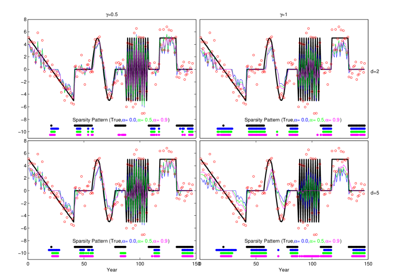
Figure 5: Simulation Results. Ground truth (black line), observations (red circles), and fitted models (blue line, $\rho=0$; green line, $\alpha=.5$; magenta line, $\alpha=.9$). The bottom of each plot shows the estimated sparsity pattern for the ground truth and estimates, with corresponding color coding. We observe that shrinkage is controlled by $\lambda$ and smoothness in the estimated sparsity pattern by $d$.

We immediately notice that the model provides shrinkage in the estimates, as controlled by $\gamma$. In addition, the ability of the model to detect sparsity is dependent on the correlation structure. For example, when the ground truth consists of alternating values $+5$ and $-5$, and $\alpha=.9$, the model fits this section as being sparse, due to the lack of smoothness. We also notice that the parameter $d$ has two major implications. Firstly, it creates smoothness and stability in the estimate of sparsity structure. Secondly, because the model is fit online and hence the model is in some sense a filter, there is a slight delay in detecting sparsity patterns, the size of which increases with $d$.

We now sample from the posterior distribution through the aforementioned sequential Monte Carlo algorithm, using $1000$ iterations of the particle independent Metropolis-Hastings algorithm (Andrieu et al.,, 2010), each with $1000$ particles. We set $\sigma_{t}$, $\nu$, and $\gamma$ to $1$, and $\delta$ to $0.01$. Also, to induce moderate correlation, we select $\alpha=0.8$, and for the temporal correlation in $d$, set $\rho=0.9$. These choices were made to demonstrate the estimation of $d$, although we emphasize that depending on the circumstances and model criterion other parameter choices provide wide modeling flexibility, allowing practitioners to recreate several models in the literature (Snoussi and Idier,, 2006; Griffin and Brown,, 2007; Caron and Doucet,, 2008; Griffin and Brown,, 2010), as well as build unique models which extend and bridge between these models. Figure 6 shows the resulting inference for $5$ replicates of the model. Here we see that the estimate of $d$ ranges between $2$ and $10$, dropping during time steps when the structure of the simulated time series changes. We also plot the fitted model for each replicate, where we observe that while the fully Bayesian model does not produce sparsity, it does induce shrinkage and smoothing of the process.

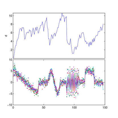
Figure 6: Results from fitting simulation data using SMC. Estimate of $d$ over time (top). Simulated observations and fitted model for $5$ replicates (bottom).

6 Modelling Stock Volatility

Stocks, as well as their derivatives, are known to alternative periods of stability and change, both on a micro and a macro scale. On a micro scale, this often occurs due to a news item or press release setting off a flurry of trading of a given asset. As an example, consider the stock price of BP oil and gas company following news of the Deepwater Horizon oil spill in 2010. Following this news, the regular day-to-day variability in the stock price increased by orders of magnitude as a constant stream of good and bad news led to an increase in trading activity. On a macro scale, this is often due to crashes, or corrections, in the market. As an example, consider the 2000 tech bubble, or the 2008 stock market crash, which both led to massive changes in the stock market as a whole.

Stock price time series are freely available from numerous sources such as Yahoo! and others, and we study a collection of stock and derivatives which we suspect would exhibit interesting effects in their prices over the period 1998 to 2011. The first stock we study is BP; as mentioned earlier, we expect to observe massive variability following the 2010 oil spill. We similarly follow OIL, iPath’s S&P Crude Oil Index. Conversely, we look at PowerShares’ Crude Oil Short (SZO), to study the effect of shorting the price of crude oil. The next asset we study is XCI, the Amex Computer Technology Index, in the hopes of observing activity from the 2000 tech bubble. Next we turn to the real estate market, as measured through ProLogis (PLD), a real estate investment trust which began in 2006, with particular interest in the 2008 market crash. These five stocks, indexes, and derivatives constitute the core of our study.

We begin by plotting the monthly change in the previously mentioned stocks and derivatives in Figure 7, where we see significant volatility in the technology sector in the early 2000’s, and similar volatility in all sectors during the 2008 recession and recovery.

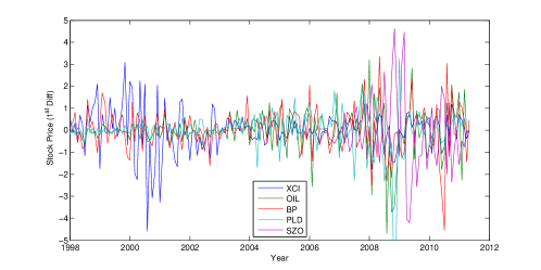
Figure 7: First differences of a portfolio of stocks and derivatives. Note the similarities with realizations from the model (Figure 4). From this plot, it is difficult to decipher major trends from noise. In contrast, see Figure 8.

One pattern of immediate note is that of SZO, the PowerShares’ Crude Oil Short, which as expected reacts contrary to the other assets during the 2008 recession.

We now attempt to model these volatilities directly, using parameters $d=0,3,6,12$, $\nu=(d+2)/2$, $\delta=0$, $\gamma=0.1,.5,1$, and $\alpha=.5$. Figure 8 plots the filtered time series for the chosen ranges of $\gamma$ and $d$, where we see that for moderate values of these parameters (namely, the two center panels), we are able to isolate significant events, such as the early 2000’s tech bubble and the 2008 recession, particularly in the housing market.

Figure 8: Model fit of first differences of a portfolio of stocks and derivatives. Note the effects of the early 2000’s tech bubble in the technology index (XCI), the 2008 housing market crash in the real estate investment trust (PLD), and the 2010 oil spill on the BP stock.

Taking a closer look at the real estate market, we now consider the very practical problem of building a portfolio in the situation where one is already largely invested in the real estate market, namely through home ownership. Specifically, the casual investor who owns their own home and wishes to diversify should aim to build a portfolio with little correlation to the housing market in case of another housing crisis. Modifying the problem slightly to regress the remaining four assets against PLD, the housing index, we calculate the regression coefficients $\beta_{PLD}$ for each time series, plotting them in Figure 9.

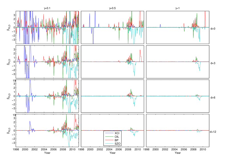
Figure 9: Regression coefficients of a portfolio of stocks and derivatives regressed on PLD. Note that as $d$ increases, the estimation of the coefficients is stabilized.

We note immediately that for small $\gamma$ and $d$ (the top left panel), it appears that all assets are highly correlated with the housing market. As we induce shrinkage and sparsity, however, we notice that the technology index, XCI, disappears. As expected, the derivative which is short on oil (SZO) is negatively correlated with the housing market during the housing collapse in 2008. Conversely, the remaining two variables are positively correlated during the crash. Using these results, one might choose to diversify their investment in their house with technology stocks, or as an alternative to hedging the housing market directly might instead hedge the price of crude oil.

7 Discussion and Extensions

The dependency structure of the $\beta_{j,1:T}$ is a d-order Markov model, which is a decomposable graph structure. The construction proposed in this paper could be generalized to any dependence structure that is given by a decomposable graph (Lauritzen,, 1996), where the joint distribution on cliques of the graph is generalized hyperbolic. This would enable one to consider dependencies, for example, on rooted trees.

In this paper, we have proposed a novel approach for conducting dynamically sparse Bayesian regression. Built on the class of multivariate generalized hyperbolic distributions, the proposed method generalized many existing approaches for tackling this problem, while providing added modeling flexibility. Inference on this class of models may be conducted exactly using MCMC methods, in particular the particle independent Metropolis-Hastings algorithm, or approximate but sparse approximations may be built around MAP estimator, using overlapping group lasso techniques or the EM algorithm.

The proposed class of models is well-suited to modeling stock volatility data, as the structure of the multivariate generalized hyperbolic distribution induces alternating periods of large and small volatility as observed daily market fluctuations. We demonstrate how, through this class of models, one is able to isolate large-scale variation in stock price volatility to build a conservative and robust portfolio of uncorrelated assets.

References

- Andrews and Mallows, (1974) Andrews, D. and Mallows, C. (1974). Scale mixtures of normal distributions. Journal of the Royal Statistical Society. Series B (Methodological), pages 99–102.
- Andrieu et al., (2010) Andrieu, C., Doucet, A., and Holenstein, R. (2010). Particle Markov chain Monte Carlo methods. Journal of the Royal Statistical Society B, 72:269–342.
- Angelosante and Giannakis, (2009) Angelosante, D. and Giannakis, G. (2009). RLS-weighted lasso for adaptive estimation of sparse signals. In International Conference on Acoustics, Speech and Signal Processing (ICASSP).
- Angelosante et al., (2009) Angelosante, D., Grossi, E., and Giannakis, G. (2009). Compressed sensing of time-varying signals. In 16th International Conference on Digital Signal Processing.
- Barndorff-Nielsen and Shephard, (2001) Barndorff-Nielsen, O. and Shephard, N. (2001). Non-Gaussian Ornstein-Uhlenbeck-based models and some of their uses in financial economics. Journal of the Royal Statistical Society B, 63:167–241.
- Bornn et al., (2010) Bornn, L., Gottardo, R., and Doucet, A. (2010). Grouping priors and the Bayesian elastic net. Technical report, Department of Statistics, University of British Columbia.
- Caron and Doucet, (2008) Caron, F. and Doucet, A. (2008). Sparse Bayesian nonparametric regression. In International Conference on Machine Learning.
- Dempster et al., (1977) Dempster, A., Laird, N., and Rubin, D. (1977). Maximum likelihood from incomplete data via the em algorithm. Journal of the Royal Statistical Society. Series B (Methodological), pages 1–38.
- Doucet et al., (2001) Doucet, A., de Freitas, N., and Gordon, N., editors (2001). Sequential Monte Carlo Methods in practice. Springer-Verlag.
- Griffin and Brown, (2007) Griffin, J. and Brown, P. (2007). Bayesian adaptive lassos with non-convex penalization. Technical report, University of Kent.
- Griffin and Brown, (2010) Griffin, J. and Brown, P. (2010). Inference with normal-gamma prior distributions in regression problems. Bayesian Analysis, 5:171–188.
- Jacob et al., (2009) Jacob, L., Obozinski, G., and Vert, J. (2009). Group lasso with overlap and graph lasso. In Proceedings of the 26th Annual International Conference on Machine Learning, pages 433–440. ACM.
- Kalli and Griffin, (2012) Kalli, M. and Griffin, J. (2012). Time-varying sparsity in dynamic regression models. Technical report, University of Kent.
- Kyung et al., (2010) Kyung, M., Gill, J., Ghosh, M., and Casella, G. (2010). Penalized regression, standard errors, and Bayesian lassos. Bayesian Analysis, 5:369–412.
- Lauritzen, (1996) Lauritzen, S. (1996). Graphical Models. Oxford University Press.
- Lee et al., (2010) Lee, A., Caron, F., Doucet, A., and Holmes, C. (2010). A hierarchical Bayesian framework for constructing sparsity-inducing priors. Technical report. Arxiv preprint arXiv:1009.1914.
- Li and Lin, (2010) Li, Q. and Lin, N. (2010). The Bayesian elastic net. Bayesian Analysis, 5:151–170.
- Mitchell and Beauchamp, (1988) Mitchell, T. and Beauchamp, J. (1988). Bayesian variable selection in linear regression (with discussion). Journal of the American Statistical Association, 83:1023–1036.
- Nakajima and West, (2011) Nakajima, J. and West, M. (2011). Bayesian analysis of latent threshold dynamic models. Technical report, Department of Statistical Science, Duke University.
- Park and Casella, (2008) Park, T. and Casella, G. (2008). The Bayesian lasso. Journal of the American Statistical Association, 103:681–686.
- Raman et al., (2009) Raman, S., Fuchs, T., Wild, P., Dahl, E., and Roth, V. (2009). The bayesian group-lasso for analyzing contingency tables. In Proceedings of the 26th Annual International Conference on Machine Learning, pages 881–888. ACM.
- Sejdinović et al., (2010) Sejdinović, D., Andrieu, C., and Piechocki, R. (2010). Bayesian sequential compressed sensing in sparse dynamical systems. In Forty-Eighth Annual Allerton Conference, USA.
- Snoussi and Idier, (2006) Snoussi, H. and Idier, J. (2006). Bayesian blind separation of generalized hyperbolic processes in noisy and underdeterminate mixtures. IEEE Transactions on Signal Processing, 54(9):3257–3269.
- Tibshirani, (1996) Tibshirani, R. (1996). Regression shrinkage and selection via the Lasso. Journal of the Royal Statistical Society B, 58:267–288.
- Tipping, (2001) Tipping, M. (2001). Sparse Bayesian learning and the relevance vector machine. Journal of Machine Learning Research, 211-244:211–244.
- Vaswani, (2008) Vaswani, N. (2008). Kalman filtered compressed sensing. In IEEE International Conference on Image Processing.
- West, (1987) West, M. (1987). On scale mixtures of normal distributions. Biometrika, 74(3):646–648.
- Yuan and Lin, (2006) Yuan, M. and Lin, Y. (2006). Model selection and estimation in regression with grouped variables. Journal of the Royal Statistical Society B, 68:49–67.
- Zhang et al., (2007) Zhang, J., Lin, M., Liu, J., and Chen, R. (2007). Lookahead and piloting strategies for variable selection. Statistica Sinica, 17(3):985.
- Ziniel et al., (2010) Ziniel, J., Potter, L., and Schniter, P. (2010). Tracking and smoothing of time-varying sparse signals via approximate belief propagation. In Forty-Fourth Asilomar Conference on Signals, Systems and Computers, Pacific Grove, CA.