Parameter Estimation of Type-II Hybrid Censored Weighted Exponential Distribution

Abstract

A hybrid censoring scheme is a mixture of Type-I and Type-II censoring schemes. We study the estimation of parameters of weighted exponential distribution based on Type-II hybrid censored data. By applying EM algorithm, maximum likelihood estimators are evaluated. Also using Fisher infirmation matrix asymptotic confidence intervals are provided. By applying Markov Chain Monte Carlo techniques Bayes estimators, and corresponding highest posterior density confidence intervals of parameters are obtained. Monte Carlo simulations to compare the performances of the different methods is performed and one data set is analyzed for illustrative purposes.
 
Keywords: Asymptotic distribution, EM algorithm, Markov Chain Monte Carlo, Hybrid censoring, Bayes estimators, Type-I censoring, Type II censoring, Maximum likelihood estimators
 
Mathematics Subject Classification: 62F10, 62F15, 62N02

1 Introduction

Type-I and Type-II censoring schemes are two most popular censoring schemes which are used in practice. They can be briefly described as follows. Suppose $n$ units are put on a life test. In Type-I censoring, the test is terminated when a pre-determined time, $T$, on test has been reached, and failures after time $T$ are not observed. In Type-II censoring, the test is terminated when a pre-chosen number, $R$, out of $n$ items has failed. It is also assumed that the failed items are not replaced. So, in Type-I censoring scheme, the number of failures is random and in Type-II censoring scheme, the experimental time is random.

A hybrid censoring scheme is a mixture of Type-I and Type-II censoring schemes and it can be described as follows. Suppose $n$ identical units are put to test. The test is finished when a pre-selected number $R$ out of $n$ items are failed, or when a pre-determined time $T$ on the test has been obtained. From now on, we call this Type-I hybrid censoring scheme and this scheme has been used as a reliability acceptance test in [24]. This censoring scheme was introduced by Epstin [12], he also studied the life testing data under the assumption of exponential distribution with mean life $\theta$. Epstein [12] proposed two-sided confidence intervals for $\theta$ without any formal proof. Fairbanks et al. [13] moderated partly the proposition of Epstein [12] and suggested a simple set of confidence intervals. Chen and Bhattacharya [3] earned the exact distribution of the conditional maximum likelihood estimator (MLE) of $\theta$ and implied a one-sided confidence interval. Childs et al. [5] proposed some simplifications of the exact distribution. From the Bayesian point of view, Drapper and Guttmann [8] studied the same problem, and reached a two-sided credible interval of the mean lifetime based on the gamma prior. Comparison of the different methods using Monte Carlo simulations, can be found in Gupta and Kundu [17]. For some related work, one may refer to Ebrahimi [10, 11], Jeong et al. [18], Childs et al. [5], Kundu [19], Banerjee and Kundu [1], Kundu and Pradhan [20], Dube et al. [9] and the references cited there.

One of the disadvantages of Type-I hybrid censoring scheme is that there may be very few failures occurring up to the pre-fixed time $T$. Because of this, Childs et al. [5] proposed a new hybrid censoring scheme known as Type-II hybrid censoring scheme which can be described as follows. Put $n$ identical items on test, and then stop the experiment at the random time $T^{*}=\mbox{max}\{x_{R:n},T\}$ , where $R$, and $T$ are prefixed numbers and $x_{R:n}$ indicates the time of $R$th failure in a sample of size $n$. Under the Type-II hybrid censoring scheme, we have one of the following three types of observations:
Case I: $\{x_{1:n}<\cdots<x_{R:n}\}$ if $x_{R:n}>T.$
Case II: $\{x_{1:n}<\cdots<x_{d:n}<T<x_{d+1:n}\}$ if $R\leq d<n$ and $x_{d:n}<T<x_{d+1:n}.$
Case III: $\{x_{1:n}<\cdots<x_{n:n}<T\},$
where $x_{1:n}<\cdots<x_{R:n}$ denote the observed ordered failure times of the experimental units. A schematic illustration of the hybrid censoring scheme is presented in Figure 1.

In this article, we consider the analysis of Type-II hybrid censored lifetime data when the lifetime of each experimental unit follows a two-parameter weighted exponential (WE) distribution. This distribution was originally proposed by Gupta and Kundu [15]. The two-parameter WE distribution with the shape and scale parameters $\alpha>0$ and $\lambda>0$, respectively, has the probability density function (pdf) as:

$$f_{WE}(x;\alpha,\lambda)=\frac{\alpha+1}{\alpha}\lambda e^{-\lambda x}(1-e^{-\alpha\lambda x});~{}~{}~{}~{}~{}~{}x>0.$$ (1.1)

We denote a two-parameter WE distribution with the pdf (1.1) by $WE(\alpha,\lambda)$ and the corresponding cumulative distribution function (cdf) by $F_{WE}(x;\alpha,\lambda)$.

The aim of this article is two fold. First, we try to earn the MLE’s of the unknown parameters. It is observed that the maximum likelihood estimators can be obtained implicitly by solving two nonlinear equations, but they cannot be obtained in closed form. So MLE’s of parameters are derived numerically. Newton-Raphson algorithm is one of the standard methods to determine the MLE’s of the parameters. To employ the algorithm, second derivatives of the log-likelihood are required for all iterations. The EM algorithm is a very powerful tool in handling the incomplete data problem see Dempster et al. [6] and McLachlan and Krishnan [23]. Then we use the EM algorithm to compute the MLE’s. We also evaluate the observed Fisher information matrix using the missing information principle which have been used to obtained asymptotic confidence intervals of the unknown parameters. The second aim of this article is to provide the Bayes inference for the unknown parameters for Type-II hybrid censored data. It is observed that Bayes estimators can not be obtained explicitly, we provide two approximations namely Lindley’s approximation and Gibbs sampling procedure. So we use the Gibbs sampling procedure to compute the Bayes estimators, and the HPD confidence intervals. We compare the performances of the different methods by Monte Carlo simulations, and for illustrative purposes we have analyzed one real data set.

The rest of the article is arranged as follows. In Section 2, we provide The MLE’s of the unknown parameters. Fisher information matrix is evaluated in Section 3. Using Lindley’s approximation and Gibbs sampling we obtain Bayes estimators and HPD confidence intervals for the parametes in Section 4. Simulation results are presented in section 5. We verify our theoretical results via analyzing data set in Section 6.

2 Maximum likelihood estimators

In this section, we study MLEs of the model parameters $\alpha$ and $\lambda$ for $\mbox{WE}(\alpha,\lambda)$ distribution with density function:

$$f(x)=\frac{\alpha+1}{\alpha}\lambda e^{-\lambda x}(1-e^{-\alpha\lambda x}):~{}\alpha,\lambda,x>0.$$

For simplicity, we apply a re-parametrization as $\alpha$ and $\beta=\alpha\lambda$. By this, the $\mbox{WE}(\alpha,\lambda)$ distribution can be written as:

$$f(x)=\frac{\alpha+1}{\alpha^{2}}\beta e^{-\frac{\beta}{\alpha}x}(1-e^{-\beta x}):~{}\alpha,\beta,x>0.$$ (2.2)

The likelihood function in Case I is given by

$$L(\alpha,\lambda)=\frac{n!}{(n-R)!}\Pi_{i=1}^{R}f(x_{i})(1-F(x_{(R)}))^{(n-R)},$$ (2.3)

for Case II,

$$L(\alpha,\lambda)=\frac{n!}{(n-d)!}\Pi_{i=1}^{d}f(x_{i})(1-F(T))^{(n-d)},$$ (2.4)

and for case III,

$$L(\alpha,\lambda)=\Pi_{i=1}^{n}f(x_{i}),$$ (2.5)

where $f(x)$ is presented by (2.2), so

$$F(x)=1-\frac{1}{\alpha}e^{-\frac{\beta}{\alpha}x}(\alpha+1-e^{-\beta x}).$$

We present likelihood functions (2.3), (2.4) and (2.5) by:

$$L(\alpha,\lambda)=\frac{n!}{(n-r)!}\Pi_{i=1}^{r}f(x_{i})(1-F(c))^{(n-r)},$$ (2.6)

where

$$r=\left\{\begin{array}[]{rl}R&\text{for Case I}\\ d&\text{for Case II}\\ n&\text{for Case III},\end{array}\right.$$ (2.7)

and

$$c=\left\{\begin{array}[]{rl}x_{R:n}&\text{for Case I}\\ T&\text{for Cases II and III.}\end{array}\right.$$ (2.8)

Taking the logarithm of Equation 2.6, we obtain

$$l(\alpha,\lambda)=r\ln(\alpha+1)-(n+r)\ln(\alpha)+r\ln(\beta)-\frac{\beta}{\alpha}\sum_{i=1}^{r}x_{i}+\sum_{i=1}^{r}{\ln(1-e^{-\beta x_{i}})}$$

$$+(n-r)(-\frac{\beta}{\alpha})c+(n-r)\ln(\alpha+1-e^{-\beta c}),$$ (2.9)

then the normal equations are

$$\left\{\begin{array}[]{c}\frac{\partial l}{\partial\alpha}=\frac{r}{\alpha+1}-\frac{n+r}{\alpha}+\frac{\beta}{\alpha^{2}}(\sum_{i=1}^{r}x_{i}+(n-r)c)+\frac{(n-r)}{\alpha+1-e^{-\beta c}}\\ \frac{\partial l}{\partial\beta}=\frac{r}{\beta}-\frac{1}{\alpha}(\sum_{i=1}^{r}x_{i}+(n-r)c)+\sum_{i=1}^{r}\frac{x_{i}e^{-\beta x_{i}}}{1-e^{-\beta x_{i}}}+(n-r)\frac{ce^{-\beta c}}{\alpha+1-e^{-\beta c}}.\end{array}\right.$$ (2.10)

Maximum likelihood estimators can be secured by solving these equations, but they cannot be expressed explicitly. So we use EM algorithm to compute them. The advantage of this method is that it is convergence for any initial value fast enough.

2.1 EM algorithm

The EM algorithm, originally proposed by Dempster et al. [6], is a very powerful tool for handling the incomplete data problem.
Let us symbolize the observed and the censored data by $X=(X_{1:n},\cdots,X_{r:n})$ and $Z=(Z_{1},\cdots,Z_{n-r})$, respectively. Here for a given r, $(Z_{1},\cdots,Z_{n-r})$ are not observable. The censored data vector $Z$ can be thought of as missing data. The combination of $W=(X,Z)$ forms the whole data set. In next we follow the method Kundu and Pradhan [20] for missing data introducing.
If we denote the log-likelihood function of the uncensored data set by

$$l_{c}(\alpha,\beta)=n\ln(\alpha+1)-2n\ln(\alpha)+n\ln(\beta)-\frac{\beta}{\alpha}\left(\sum_{i=1}^{r}X_{i}+\sum_{i=1}^{n-r}Z_{i}\right)$$

$$+\left(\sum_{i=1}^{r}{\ln(1-e^{-\beta x_{i}})}+\sum_{i=1}^{r}{\ln(1-e^{-\beta z_{i}})}\right).$$ (2.11)

For the E-step of the EM algorithm, one needs to compute the pseudo log-likelihood function as $l_{s}(\alpha,\beta)=E(l_{c}(\alpha,\beta|X)).$ Therefor,

$$l_{s}(\alpha,\beta)=n\ln(\alpha+1)-2n\ln(\alpha)+n\ln(\beta)-\frac{\beta}{\alpha}\left(\sum_{i=1}^{r}X_{i}\right)+\sum_{i=1}^{r}{\ln(1-e^{-\beta x_{i}})}$$

$$-\frac{\beta}{\alpha}(n-r)A(c;\alpha,\beta)+(n-r)B(c;\alpha,\beta),$$

where

$$A[c;\alpha,\beta]=E(Z_{i}|Z_{i}>c)~{}~{}\mbox{and}~{}~{}B(c;\alpha,\beta)=E[\ln(1-e^{-\beta Z_{i}})|Z_{i}>c],$$

and they are obtained in Appendix A.

Now the M-step includes the maximization of the pseudo log-likelihood function 2.11. Therefore, if at the kth stage, the estimation of $(\alpha,\beta)$ is $(\hat{\alpha}_{k},\hat{\beta}_{k})$, then $(\hat{\alpha}_{k+1},\hat{\beta}_{k+1})$ can be obtained by maximizing

$$g(\alpha,\beta)=n\ln(\alpha+1)-2n\ln(\alpha)+n\ln(\beta)-\frac{\beta}{\alpha}\left(\sum_{i=1}^{r}X_{i}\right)+\sum_{i=1}^{r}{\ln(1-e^{-\beta x_{i}})}$$

$$-\frac{\beta}{\alpha}(n-r)A(c;\hat{\alpha}_{k},\hat{\beta}_{k})+(n-r)B(c;\hat{\alpha}_{k},\hat{\beta}_{k})$$ (2.12)

Note that the maximization of 2.12 can be earned quite effectively by the similar method proposed by Gupta and Kundu [16]. First, $\hat{\beta}_{k+1}$ can be obtain by solving a fixed-point type equation

$$h(\beta)=\beta.$$

The function $h(\beta)$ is defined

$$h(\beta)=n\left[\frac{B}{\hat{\alpha}(\beta)}-\sum_{i=1}^{r}\frac{x_{i}e^{-\beta x_{i}}}{1-e^{-\beta x_{i}}}\right]^{-1}$$

where

$$B=\sum_{i=1}^{r}x_{i}+(n-r)A(c,\hat{\alpha}_{k},\hat{\beta}_{k})$$

and

$$\hat{\alpha}(\beta)=\frac{\sqrt{(\beta B-2n)^{2}+4n\beta B}+(\beta B-2n)}{2n}.$$

One can follow iteration method. Once $\hat{\beta}_{k+1}$ is determined, $\hat{\alpha}_{k+1}$ can be evaluated as $\hat{\alpha}_{k+1}=\hat{\alpha}(\hat{\beta}_{k+1})$.

For the estimation of $\lambda$, we can use the invariance property maximum likelihood estimators and obtain $\hat{\lambda}$ as follow:

$$\hat{\lambda}=\frac{\hat{\beta}}{\hat{\alpha}}.$$

3 Fisher Information matrices

One of the advantages of using EM algorithm is that presents a measure of information in censored data through the missing information principle. Louis [22] improved a procedure for extracting the observed information matrix. In this section, we display the observed Fisher information matrix by using the missing value principles of Louis [22]. The observed Fisher information matrix can be used to build the asymptotic confidence intervals.
Using the notations: $\theta=(\alpha,\beta)$, X=observed data, W=complete data, $I_{X}(\theta)$=observed information, $I_{W}(\theta)$=complete information and $I_{W|X}(\theta)$=missing information, follow the relation to

$$I_{X}(\theta)=I_{W}(\theta)-I_{W|X}(\theta),$$ (3.13)

to evaluate $I_{X}(\theta).$
Complete information and the missing information are given respectively as:

$$I_{W}(\theta)=-E\left[\frac{\partial^{2}L_{c}(W;\theta)}{\partial\theta^{2}}\right]$$

and

$$I_{W|X}(\theta)=-(n-r)E\left[\frac{\partial^{2}\ln f_{Z}(z|y,\theta)}{\partial\theta^{2}}\right].$$ (3.14)

As the dimension of $\theta$ is 2, $I_{X}(\theta)$ and $I_{W|X}(\theta)$ are both of the order $2\times 2$.

The elements of matrix $I_{W}(\theta)$ for complete data set are presented in Gupta and Kundu [15]. They re-parametrized $\mbox{WE}(\alpha,\lambda)$ distribution as $\lambda$ and $\beta=\alpha\lambda$.
We report $I_{W}(\theta)$ which have been evaluated by them here as:

$$I_{W}(\theta)=\left[\begin{array}[]{cc}a_{11}&a_{12}\\ a_{21}&a_{22}\end{array}\right]$$

where

$$a_{11}=\frac{n}{(\beta+\lambda)^{2}}+\frac{n}{\lambda^{2}}.$$

$$a_{12}=a_{21}=\frac{n}{(\beta+\lambda)^{2}}.$$

$$a_{22}=\frac{n}{(\beta+\lambda)^{2}}-\frac{n}{\beta^{2}}+\frac{n\lambda(\beta+\lambda)A}{\beta^{4}},$$

in which $\displaystyle A=\int_{0}^{1}\frac{(\ln(1-y))^{2}(1-y)^{\frac{\lambda}{\beta}}}{y}dy.$
On the other hand, with the above re-parametrization and by using (3.14), one can easily verify

$$I_{W|X}(\theta)=(n-r)\left[\begin{array}[]{cc}b_{11}(c;\alpha,\beta)&b_{12}(c;\alpha,\beta)\\ b_{21}(c;\alpha,\beta)&b_{22}(c;\alpha,\beta)\end{array}\right],$$

where

$$b_{11}(c;\alpha,\beta)=\frac{1}{(\beta+\lambda)^{2}}+\frac{2\beta}{\lambda^{3}(\frac{\beta}{\lambda}+1-e^{-\beta c})}-\frac{\beta^{2}}{\lambda^{4}(\frac{\beta}{\lambda}+1-e^{-\beta c})^{2}}.$$

$$b_{12}(c;\alpha,\beta)=b_{21}(c;\alpha,\beta)=\frac{1}{(\beta+\lambda)^{2}}-\frac{1}{\lambda^{2}(\frac{\beta}{\lambda}+1-e^{-\beta c})}+\frac{\beta(\frac{1}{\lambda}+ce^{-\beta c})}{\lambda^{2}(\frac{\beta}{\lambda}+1-e^{-\beta c})^{2}}.$$

$$b_{22}(c;\alpha,\beta)=\frac{1}{(\beta+\lambda)^{2}}-\frac{c^{2}e^{-\beta c}}{\frac{\beta}{\lambda}+1-e^{-\beta c}}-\frac{(\frac{1}{\lambda}+c-e^{-\beta c})^{2}}{(\frac{\beta}{\lambda}+1-e^{-\beta c})^{2}}+\frac{(\beta+\lambda)B}{\beta^{3}e^{-\lambda c}(\frac{\beta}{\lambda}+1-e^{-\beta c})},$$

in which $B=\int_{1-e^{-\beta c}}^{1}\frac{(\ln(1-y))^{2}(1-y)^{\frac{\lambda}{\beta}}}{y}dy.$

Now, $I_{X}(\theta)$ can be computed by (3.13). The asymptotic variance-covariance matrix of $\hat{\theta}$ can be obtained by inverting $I_{X}(\theta)$. We use this matrix to secure the asymptotic confidence intervals for $\lambda$ and $\beta$. To obtain the asymptotic confidence interval for $\alpha$, we use the non-parametric bootstrap method [25].

4 Bayes Estimators and Confidence Intervals

In this section, we study Bayes estimators for parameters $\alpha$ and $\lambda$ under symmetric loss functions. A very well known symmetric loss function is the squared error which is defined as: $L(f(\mu),\hat{f}(\mu))=(\hat{f}(\mu)-f(\mu))^{2},$ with $\hat{f}(\mu)$ being an estimate of $f(\mu)$. Here $f(\mu)$ denotes some function of $\mu$. Bayes estimators, say $\hat{f}_{Bayes}(\mu)$, is evaluated by the posterior mean of $f(\mu)$.

Let $x=(x_{1:n},\cdots,x_{r:n})$ be an observed sample from the hybrid censoring scheme, drawn from a $\mbox{WE}(\alpha,\lambda)$ distribution. We apply re-parametrization as $\alpha$ and $\beta=\alpha\lambda$. So the likelihood function becomes

$$L(\alpha,\beta|\b{x})\varpropto\frac{(\alpha+1)^{r}}{\alpha^{n+r}}\beta^{r}e^{-\frac{\beta}{\alpha}\left(\sum_{i=1}^{r}x_{i}+c(n-r)\right)}(\alpha+1-e^{-\beta c})^{n-r}\Pi_{i=1}^{r}(1-e^{-\beta x_{i}}),$$

and $\log$-likelihood function:

$$l(\alpha,\beta|\b{x})=r\log(\alpha+1)-(n+r)\log\alpha+r\log(\beta)-\frac{\beta}{\alpha}\left(\sum_{i=1}^{r}x_{i}+c(n-r)\right)$$

$$+(n-r)\log(\alpha+1-e^{-\beta c})+\sum_{i=1}^{r}\log(1-e^{-\beta x_{i}}).$$ (4.15)

It is assumed that $\beta$ and $\alpha$ have the following independent gamma priors:

$$\pi_{1}(\beta)\varpropto\beta^{w_{2}-1}e^{-\beta w_{1}},~{}~{}~{}~{}~{}~{}\beta>0,$$

$$\pi_{2}(\alpha)\varpropto\alpha^{w_{4}-1}e^{-\alpha w_{3}},~{}~{}~{}~{}~{}~{}\alpha>0.$$

So, the joint prior distribution of $\alpha$ and $\beta$ is of the form

$$\pi(\alpha,\beta)\varpropto\alpha^{w_{4}-1}e^{-\alpha w_{3}}\beta^{w_{2}-1}e^{-\beta w_{1}},~{}~{}~{}~{}~{}~{}~{}\alpha>0,~{}\beta>0,~{}w_{1}>0,~{}w_{2}>0,~{}w_{3}>0,~{}w_{4}>0.$$

Then the posterior distribution $\alpha$ and $\beta$ can be written as

$$\pi(\alpha,\beta|\b{x})=\frac{1}{k}\alpha^{w_{4}-n-r-1}\beta^{w_{2}+r-1}(\alpha+1)^{r}e^{-\alpha w_{3}}e^{-\beta w_{1}}e^{-\frac{\beta}{\alpha}\left(\sum_{i=1}^{r}x_{i}+c(n-r)\right)}$$

$$\times(\alpha+1-e^{-\beta c})^{n-r}\Pi_{i=1}^{r}(1-e^{-\beta x_{i}})$$ (4.16)

where

$$k=\int_{0}^{\infty}\int_{0}^{\infty}\alpha^{w_{4}-n-r-1}\beta^{w_{2}+r-1}(\alpha+1)^{r}e^{-\alpha w_{3}}e^{-\beta w_{1}}e^{-\frac{\beta}{\alpha}\left(\sum_{i=1}^{r}x_{i}+c(n-r)\right)}$$

$$\times(\alpha+1-e^{-\beta c})^{n-r}\Pi_{i=1}^{r}(1-e^{-\beta x_{i}})d\alpha d\beta.$$

Now the Bayes estimators of $\alpha$ and $\beta$ under the squared error loss function L are respectively obtained as:

$$\hat{\alpha}_{Bayes}=E[\alpha|\b{x}]=\frac{1}{k}\int_{0}^{\infty}\int_{0}^{\infty}\alpha^{w_{4}-n-r}\beta^{w_{2}+r-1}(\alpha+1)^{r}e^{-\alpha w_{3}}e^{-\beta w_{1}}$$

$$\times e^{-\frac{\beta}{\alpha}\left(\sum_{i=1}^{r}x_{i}+c(n-r)\right)}(\alpha+1-e^{-\beta c})^{n-r}\Pi_{i=1}^{r}(1-e^{-\beta x_{i}})d\alpha d\beta,$$

and

$$\hat{\beta}_{Bayes}=E[\beta|\b{x}]=\frac{1}{k}\int_{0}^{\infty}\int_{0}^{\infty}\alpha^{w_{4}-n-r-1}\beta^{w_{2}+r}(\alpha+1)^{r}e^{-\alpha w_{3}}e^{-\beta w_{1}}$$

$$\times e^{-\frac{\beta}{\alpha}\left(\sum_{i=1}^{r}x_{i}+c(n-r)\right)}(\alpha+1-e^{-\beta c})^{n-r}\Pi_{i=1}^{r}(1-e^{-\beta x_{i}})d\alpha d\beta.$$

Since $\lambda$ is a function of $\alpha$ and $\beta$, then one can obtain the posterior density function of $\lambda$ and so the Bayes estimator of $\lambda$ under the squared error loss function $L$ as:

$$\hat{\lambda}_{Bayes}=E[\lambda|\b{x}]=\frac{1}{k}\int_{0}^{\infty}\int_{0}^{\infty}u^{w_{4}+w_{2}-n-1}\lambda^{w_{2}+r-1}(1+u)^{r}e^{-u(w_{3}+\lambda w_{1})}$$

$$\times e^{-\lambda\left(\sum_{i=1}^{r}x_{i}+c(n-r)\right)}(u+1-e^{-\lambda uc})^{n-r}\Pi_{i=1}^{r}(1-e^{-\lambda ux_{i}})dud\lambda.$$

As these estimators can not be evaluated explicitly, so we adopt two different procedures to approximate them:

• Lindley approximation,

• MCMC method.

4.1 Lindley approximation method

In previous section, based on Type-II hybrid censored scheme we obtained the Bayes estimators of $\alpha$, $\beta$ and $\lambda$ against squared error loss function $L$. It is easily observed that theses estimators have not explicit closed forms. For these evaluation, numerical techniques are required. One of the most numerical techniques is Lindley’s method (see [21]), that for these estimators can be describe as follows. In general, Bayes estimator of $u(\alpha,\beta)$ as a function of $\alpha$ and $\beta$ is identified:

$$I(\b{x})=\frac{\int_{0}^{\infty}\int_{0}^{\infty}u(\alpha,\beta)e^{l(\alpha,\beta|\b{x})+\rho(\alpha,\beta)}d\alpha d\beta}{\int_{0}^{\infty}\int_{0}^{\infty}e^{l(\alpha,\beta|\b{x})+\rho(\alpha,\beta)}d\alpha d\beta},$$

where $l(\alpha,\beta|\b{x})$ is $\log$-likelihood function (defined by 4.15) and $\rho(\alpha,\beta)=\log\pi(\alpha,\beta)$.
By the Lindley’s method $I(\b{x})$ can be approximated as:

$$I(\b{x})=u(\hat{\alpha},\hat{\beta})+\frac{1}{2}[(\hat{u}_{\alpha\alpha}+2\hat{u}_{\alpha}\hat{\rho}_{\alpha})\hat{\sigma}_{\alpha\alpha}+(\hat{u}_{\beta\alpha}+2\hat{u}_{\beta}\hat{\rho}_{\alpha})\hat{\sigma}_{\beta\alpha}+(\hat{u}_{\alpha\beta}+2\hat{u}_{\alpha}\hat{\rho}_{\beta})\hat{\sigma}_{\alpha\beta}$$

$$+(\hat{u}_{\beta\beta}+2\hat{u}_{\beta}\hat{\rho}_{\beta})\hat{\sigma}_{\beta\beta}]+\frac{1}{2}[(\hat{u}_{\alpha}\hat{\sigma}_{\alpha\alpha}+\hat{u}_{\beta}\hat{\sigma}_{\alpha\beta})(\hat{l}_{\alpha\alpha\alpha}\hat{\sigma}_{\alpha\alpha}+\hat{l}_{\alpha\beta\alpha}\hat{\sigma}_{\alpha\beta}+\hat{l}_{\beta\alpha\alpha}\hat{\sigma}_{\beta\alpha}$$

$$+\hat{l}_{\beta\beta\alpha}\hat{\sigma}_{\beta\beta})+(\hat{u}_{\alpha}\hat{\sigma}_{\beta\alpha}+\hat{u}_{\beta}\hat{\sigma}_{\beta\beta})(\hat{l}_{\beta\alpha\alpha}\hat{\sigma}_{\alpha\alpha}+\hat{l}_{\alpha\beta\beta}\hat{\sigma}_{\alpha\beta}+\hat{l}_{\beta\alpha\beta}\hat{\sigma}_{\beta\alpha}+\hat{l}_{\beta\beta\beta}\hat{\sigma}_{\beta\beta})],$$

where $\hat{\alpha}$ and $\hat{\beta}$ are the MLE’s of $\alpha$ and $\beta$ respectively. Also, $u_{\alpha\alpha}$ is the second derivative of the function $u(\alpha,\beta)$ with the respect to $\alpha$ and $\hat{u}_{\alpha\alpha}$ valued of $u_{\alpha\alpha}$ at $(\hat{\alpha},\hat{\beta}).$ Other expressions can be calculated with following definitions:

$$\hat{l}_{\alpha\alpha}=\frac{\partial^{2}l}{\partial\alpha^{2}}\left|{}_{\alpha=\hat{\alpha},\beta=\hat{\beta}}=\frac{-r}{(\hat{\alpha}+1)^{2}}+\frac{n+r}{\hat{\alpha}^{2}}-\frac{2\hat{\beta}A}{\hat{\alpha}^{3}}-\frac{n-r}{(\hat{\alpha}+1-e^{-\hat{\beta}c})^{2}}\right.,$$

$$\hat{l}_{\alpha\beta}=\frac{\partial^{2}l}{\partial\alpha\partial\beta}\left|{}_{\alpha=\hat{\alpha},\beta=\hat{\beta}}=\hat{l}_{\beta\alpha}=\frac{A}{\hat{\alpha}^{2}}-\frac{c(n-r)e^{-\hat{\beta}c}}{(\hat{\alpha}+1-e^{-\hat{\beta}c})^{2}}\right.,$$

$$\hat{l}_{\alpha\beta\alpha}=\frac{\partial^{3}l}{\partial\alpha\partial\beta\partial\alpha}\left|{}_{\alpha=\hat{\alpha},\beta=\hat{\beta}}=\hat{l}_{\beta\alpha\alpha}=\frac{\partial^{3}l}{\partial\beta\partial\alpha^{2}}\left|{}_{\alpha=\hat{\alpha},\beta=\hat{\beta}}=\frac{-2A}{\hat{\alpha}^{3}}+\frac{2c(n-r)e^{-\hat{\beta}c}}{(\hat{\alpha}+1-e^{-\hat{\beta}c})^{3}}\right.\right.,$$

$$\hat{l}_{\alpha\alpha\alpha}=\frac{\partial^{3}l}{\partial\alpha^{3}}\left|{}_{\alpha=\hat{\alpha},\beta=\hat{\beta}}=\frac{2r}{(\hat{\alpha}+1)^{3}}-\frac{2(n+r)}{\hat{\alpha}^{3}}+\frac{6\hat{\beta}A}{\hat{\alpha}^{4}}+\frac{2(n-r)}{(\hat{\alpha}+1-e^{-\hat{\beta}c})^{3}}\right.,$$

where $A=\sum_{i=1}^{r}x_{i}+(n-r)c,$

$$\hat{l}_{\alpha\beta\beta}=\frac{\partial^{3}l}{\partial\alpha\partial\beta^{2}}\left|{}_{\alpha=\hat{\alpha},\beta=\hat{\beta}}=\hat{l}_{\beta\alpha\beta}=\frac{\partial^{3}l}{\partial\beta\partial\alpha\partial\beta}\left|{}_{\alpha=\hat{\alpha},\beta=\hat{\beta}}=\frac{c^{2}(n-r)e^{-\hat{\beta}c}(\hat{\alpha}+1+e^{-\hat{\beta}c})}{(\hat{\alpha}+1-e^{-\hat{\beta}c})^{3}}\right.\right.,$$

$$\hat{l}_{\beta\beta}=\frac{\partial^{2}l}{\partial\beta^{2}}\left|{}_{\alpha=\hat{\alpha},\beta=\hat{\beta}}=\frac{-r}{\hat{\beta}^{2}}-\frac{c^{2}(n-r)(\hat{\alpha}+1)e^{-\hat{\beta}c}}{(\hat{\alpha}+1-e^{-\hat{\beta}c})^{2}}-\sum_{i=1}^{r}\frac{x_{i}^{2}e^{-\hat{\beta}x_{i}}}{(1-e^{-\hat{\beta}x_{i}})^{2}}\right.,$$

$$\hat{l}_{\beta\beta\alpha}=\frac{\partial^{3}l}{\partial\beta^{2}\partial\alpha}\left|{}_{\alpha=\hat{\alpha},\beta=\hat{\beta}}=\frac{c^{2}(n-r)e^{-\hat{\beta}c}(\hat{\alpha}+1+e^{-\hat{\beta}c})}{(\hat{\alpha}+1-e^{-\hat{\beta}c})^{3}}\right.,$$

$$\hskip 3.61371pt\hat{l}_{\beta\beta\beta}=\frac{\partial^{3}l}{\partial\beta^{3}}\left|{}_{\alpha=\hat{\alpha},\beta=\hat{\beta}}=\frac{2r}{\hat{\beta}^{3}}+\frac{c^{3}(n-r)(\hat{\alpha}+1)e^{-\hat{\beta}c}(\hat{\alpha}+1+e^{-\hat{\beta}c})}{(\hat{\alpha}+1-e^{-\hat{\beta}c})^{3}}+\sum_{i=1}^{r}\frac{x_{i}^{3}e^{-\hat{\beta}x_{i}}(1+e^{-\hat{\beta}x_{i}})}{(1-e^{-\hat{\beta}x_{i}})^{3}}\right.,$$

$$\hat{\rho}_{\beta}=\frac{\partial\rho}{\partial\beta}\left|{}_{\beta=\hat{\beta}}=\frac{w_{2}-1}{\hat{\beta}}-w_{1}\right.,$$

$$\hat{\rho}_{\alpha}=\frac{\partial\rho}{\partial\alpha}\left|{}_{\alpha=\hat{\alpha}}=\frac{w_{4}-1}{\hat{\alpha}}-w_{3}\right.,$$

and we have:

$$\left(\begin{array}[]{cc}\hat{\sigma}_{\alpha\alpha}&\hat{\sigma}_{\alpha\beta}\\ \hat{\sigma}_{\beta\alpha}&\hat{\sigma}_{\beta\beta}\end{array}\right)=\left(\begin{array}[]{cc}-\hat{l}_{\alpha\alpha}&-\hat{l}_{\alpha\beta}\\ -\hat{l}_{\beta\alpha}&-\hat{l}_{\beta\beta}\end{array}\right)^{-1}.$$

With the above defined expressions, we obtain the approximation Bayes estimators.
Also we have:

$$u(\alpha,\beta)=\alpha,~{}~{}~{}~{}u_{\alpha}=1,~{}~{}~{}~{}u_{\alpha\alpha}=u_{\beta}=u_{\beta\beta}=u_{\alpha\beta}=u_{\beta\alpha}=0,$$

the Bayes estimator of $\alpha$ under the squared error loss function $L$ becomes

$$\hat{\alpha}_{Bayes}=\hat{\alpha}+\frac{1}{2}[2\hat{\rho}_{\alpha}\hat{\sigma}_{\alpha\alpha}+2\hat{\rho}_{\beta}\hat{\sigma}_{\alpha\beta}+\hat{\sigma}^{2}_{\alpha\alpha}\hat{l}_{\alpha\alpha\alpha}+3\hat{\sigma}_{\alpha\alpha}\hat{\sigma}_{\alpha\beta}\hat{l}_{\beta\alpha\alpha}+2\hat{\sigma}^{2}_{\alpha\beta}\hat{l}_{\alpha\beta\beta}$$

$$+\hat{\sigma}_{\alpha\alpha}\hat{\sigma}_{\beta\beta}\hat{l}_{\beta\beta\alpha}+\hat{\sigma}_{\alpha\beta}\hat{\sigma}_{\beta\beta}\hat{l}_{\beta\beta\beta}].$$

Proceeding similarly, the Bayes estimator of $\beta$ under $L$ is given by

$$(u(\alpha,\beta)=\beta,~{}~{}~{}~{}u_{\beta}=1,~{}~{}~{}~{}u_{\alpha\alpha}=u_{\alpha}=u_{\beta\beta}=u_{\alpha\beta}=u_{\beta\alpha}=0),$$

$$\hat{\beta}_{Bayes}=\hat{\beta}+\frac{1}{2}[2\hat{\rho}_{\alpha}\hat{\sigma}_{\alpha\beta}+2\hat{\rho}_{\beta}\hat{\sigma}_{\beta\beta}+2\hat{\sigma}^{2}_{\alpha\beta}\hat{l}_{\beta\alpha\alpha}+2\hat{\sigma}_{\alpha\beta}\hat{\sigma}_{\beta\beta}\hat{l}_{\alpha\beta\beta}$$

$$+\hat{\sigma}^{2}_{\beta\beta}\hat{l}_{\beta\beta\beta}+\hat{\sigma}_{\alpha\alpha}\hat{\sigma}_{\alpha\beta}\hat{l}_{\alpha\alpha\alpha}+\hat{\sigma}_{\beta\beta}\hat{\sigma}_{\alpha\alpha}\hat{l}_{\beta\alpha\alpha}+\hat{\sigma}_{\alpha\beta}\hat{\sigma}_{\beta\beta}\hat{l}_{\beta\beta\alpha}].$$

Finally the Bayes estimator of $\lambda$ under $L$ is given by

$$(u(\alpha,\beta)=\frac{\beta}{\alpha},~{}~{}u_{\beta}=\frac{1}{\alpha},~{}~{}u_{\alpha}=\frac{-\beta}{\alpha^{2}},~{}~{}u_{\alpha\alpha}=\frac{2\beta}{\alpha^{3}},~{}~{}u_{\beta\beta}=0,~{}~{}u_{\alpha\beta}=u_{\beta\alpha}=\frac{-1}{\alpha^{2}}),$$

$$\hat{\lambda}_{Bayes}=\frac{\hat{\beta}}{\hat{\alpha}}+\frac{1}{2}[(\hat{u}_{\alpha\alpha}+2\hat{u}_{\alpha}\hat{\rho}_{\alpha})\hat{\sigma}_{\alpha\alpha}+(\hat{u}_{\beta\alpha}+2\hat{u}_{\beta}\hat{\rho}_{\alpha})\hat{\sigma}_{\beta\alpha}+(\hat{u}_{\alpha\beta}+2\hat{u}_{\alpha}\hat{\rho}_{\beta})\hat{\sigma}_{\alpha\beta}$$

$$+2\hat{u}_{\beta}\hat{\rho}_{\beta}\hat{\sigma}_{\beta\beta}]+\frac{1}{2}[(\hat{u}_{\alpha}\hat{\sigma}_{\alpha\alpha}+\hat{u}_{\beta}\hat{\sigma}_{\alpha\beta})(\hat{l}_{\alpha\alpha\alpha}\hat{\sigma}_{\alpha\alpha}+\hat{l}_{\alpha\beta\alpha}\hat{\sigma}_{\alpha\beta}+\hat{l}_{\beta\alpha\alpha}\hat{\sigma}_{\beta\alpha}$$

$$\hskip 36.135pt+\hat{l}_{\beta\beta\alpha}\hat{\sigma}_{\beta\beta})+(\hat{u}_{\alpha}\hat{\sigma}_{\beta\alpha}+\hat{u}_{\beta}\hat{\sigma}_{\beta\beta})(\hat{l}_{\beta\alpha\alpha}\hat{\sigma}_{\alpha\alpha}+\hat{l}_{\alpha\beta\beta}\hat{\sigma}_{\alpha\beta}+\hat{l}_{\beta\alpha\beta}\hat{\sigma}_{\beta\alpha}+\hat{l}_{\beta\beta\beta}\hat{\sigma}_{\beta\beta})].$$

The approximate Bayes estimators of $\alpha$, $\beta$ and $\lambda$ can be obtained using Lindley approximation, but it is not possible to construct highest posterior density (HPD) confidence intervals using this method. Therefore, we suggest the following Markov Chain Monte Carlo (MCMC) method to generate samples from the posterior density function, and in turn to obtain the Bayes estimators, and HPD confidence intervals.

4.2 Gibbs sampling

Here we study the Gibbs sampling method to draw samples from the posterior density function and then compute the Bayes estimators and HPD confidence intervals of $\alpha$, $\beta$ and $\lambda$ under the squared errors loss function.

Let $\b{x}=(x_{1:n},\cdots,x_{r:n})$ be an observed sample from the hybrid censoring scheme, drawn from a $\mbox{WE}(\alpha,\lambda)$ distribution. From (4.16), we can write the joint posterior density function of $\alpha$ and $\beta$ given $\b{x}$ as:

$$\pi(\alpha,\beta|\b{x})\propto\alpha^{w_{4}-n-r-1}\beta^{w_{2}+r-1}(\alpha+1)^{r}e^{-\alpha w_{3}}e^{-\beta w_{1}}\left\{e^{-\frac{\beta}{\alpha}\left(\sum_{i=1}^{r}x_{i}+c(n-r)\right)}\right.$$

$$\left.\times(\alpha+1-e^{-\beta c})^{n-r}\Pi_{i=1}^{r}(1-e^{-\beta x_{i}})\right\},$$ (4.17)

by this, the posterior density function of $\beta$ given $\alpha$ and $\b{x}$ is

$$\pi(\beta|\alpha,\b{x})\propto\beta^{w_{2}+r-1}e^{-\beta\left(w_{1}+\frac{\beta}{\alpha}\sum_{i=1}^{r}x_{i}+c(n-r)\right)}(\alpha+1-e^{-\beta c})^{n-r}\Pi_{i=1}^{r}(1-e^{-\beta x_{i}}).$$

Theorem 4.1

The conditional distribution of $\beta$ given $\alpha$ and $\b{x}$ is log-concave.

Proof 4.1

See Appendix, part B.

By (4.17), the posterior density function of $\alpha$ given $\beta$ and $\b{x}$ is

$$\pi(\alpha|\beta,\b{x})\propto\alpha^{w_{4}-n-r-1}(\alpha+1)^{r}e^{-\alpha w_{3}}e^{-\frac{\beta}{\alpha}\left(\sum_{i=1}^{r}x_{i}+c(n-r)\right)}(\alpha+1-e^{-\beta c})^{n-r}.$$ (4.18)

Theorem 4.2

The conditional distribution of $\alpha$ given $\beta$ and $\b{x}$ has a finite maximum point.

Proof 4.2

See Appendix, part C.

Corollary 4.1

With the help of the acceptance rejection principle (see Devroye [7] for details) and the previous theorem, the generation from (4.18) can be performed using the WE generator.

Now we use theorems 4.2 and 4.2 and pursue the idea of Geman and Geman [14], and suggest the following scheme.

• Step 1) Take some initial value of $\alpha$ and $\beta$, such as $\alpha_{0}$ and $\beta_{0}$.

• Step 2) Generate $\alpha_{i+1}$ and $\beta_{i+1}$ from $\pi(\alpha|\beta_{i},\b{x})$ and $\pi(\beta|\alpha_{i},\b{x})$.

• Step 3) Repeat Step 2, $N$ times.

• Step 4) Obtain Bayes estimators of $\alpha$ and $\beta$ with respect to a squared error loss function:

  $$\hat{\alpha}_{Bayes}=\frac{1}{N-M_{1}}\sum_{i=M_{1}+1}^{N}{\alpha_{i}}~{}~{}~{}~{}\mbox{and}~{}~{}~{}~{}\hat{\beta}_{Bayes}=\frac{1}{N-M_{2}}\sum_{i=M_{2}+1}^{N}{\beta_{i}}$$

  where $M_{1}$ and $M_{2}$ are the burn-in periods in generating of $\alpha_{i}$ and $\beta_{i}$ respectively.

• Step 5) Obtain the HPD confidence interval of $\alpha$: Order $\alpha_{1},\cdots,\alpha_{M_{1}}$ as $\alpha_{(1)}<\cdots<\alpha_{(M_{1})}$ and construct all the $100(1-\eta)\%$ confidence intervals of $\alpha$, as:

  $$(\alpha_{(1)},\alpha_{([M_{1}(1-\eta)])}),\cdots,(\alpha_{([M_{1}\eta])},\alpha_{(M_{1})}),$$

  where $[M]$ symbolizes the largest integer less than or equal to $M$. The HPD confidence interval of $\alpha$ is the shortest length interval. Similarly, we can construct a $100(1-\eta)\%$ HPD confidence interval of $\beta$.

Finally, using the idea of Chen and Shao [4], we can compute the estimation and HPD confidence interval for $\lambda$.

5 Numerical Experiments

In this section, we carry out a simulation study to compare the performance of MLE’s and Bayes estimators. In all the cases $\alpha=2.5$ and $\lambda=3$ are taken. We estimate the unknown parameters using the MLE, Bayes estimators obtained by Lindley’s approximations and also Bayes estimators obtained by using MCMC technique. We compare the performances of different estimators with MSE. We also obtain the average length of the asymptotic confidence intervals and the HPD confidence intervals.

For computing the Bayes estimators, it is assumed that $\beta$ and $\alpha$ have $\mbox{Gamma}(w_{2},w_{1})$ and $\mbox{Gamma}(w_{4},w_{3})$ priors, respectively. Moreover we use the non-informative priors of both $\beta$ and $\alpha$, by considering $w_{1}=w_{2}=w_{3}=w_{4}=0$. The Bayes estimators are computed under the squared error loss function and with respect to the above non-informative priors.

The simulation is performed for different choices of $n,~{}R,~{}T$ values. We replicate the procedure for 1000 times and report the average estimators, the MSE’s, the average asymptotic confidence intervals length and the average HPD confidence intervals length from the MCMC technique. The results are reported in Table 1-4. The first and second rows are parameter estimators of $\lambda$ and $\alpha$, respectively.

Table 1: Average estimators, corresponding MSE and average confidence (asymptotic or HPD for Gibbs) length for N=40 , T=1

	R=25	R=30	R=35
MLE	2.978(4.623)3.013	3.014(1.836)2.993	2.909(0.008)2.999
	2.575(0.029)0.945	2.574(0.028)0.985	2.578(0.027)0.814
Bayes(Lindley)	2.863(0.019)	2.968(0.019)	2.863(0.019)
	2.573(0.005)	2.570(0.005)	2.574(0.005)
Bayes(Gibbs)	2.987(0.246)1.829	2.979(0.179)1.516	2.944(0.159)1.451
	2.472(0.055)0.757	2.482(0.053)0.751	2.489(0.053)0.759

Table 2: Average estimators, corresponding MSE and average confidence (asymptotic or HPD for Gibbs) length for N=40 , T=2

	R=25	R=30	R=35
MLE	3.192(0.037)2.865	3.145(0.021)2.899	2.908(0.008)2.889
	2.624(0.046)0.972	2.591(0.033)0.891	2.585(0.032)0.894
Bayes(Lindley)	2.968(0.001)	2.968(0.001)	2.963(0.001)
	2.621(0.015)	2.576(0.006)	2.581(0.006)
Bayes(Gibbs)	3.148(0.216)1.544	3.004(0.166)1.217	2.956(0.146)1.354
	2.479(0.054)0.0752	2.482(0.054)0.748	2.481(0.053)0.758

Table 3: Average estimators, corresponding MSE and average confidence (asymptotic or HPD for Gibbs) length for N=50 , T=1

	R=35	R=40	R=45
MLE	3.287(0.083)2.669	3.079(0.006)2.667	3.041(0.002)2.735
	2.556(0.019)0.731	2.555(0.018)0.763	2.463(0.018)0.784
Bayes(Lindley)	2.979(0.000)	2.984(0.000)	2.981(0.000)
	2.554(0.003)	2.552(0.003)	2.561(0.003)
Bayes(Gibbs)	2.958(0.269)1.661	3.066(0.247)1.643	2.966(0.234)1.318
	2.484(0.054)0.759	2.485(0.054)0.757	2.485(0.052)0.757

Table 4: Average estimators, corresponding MSE and average confidence (asymptotic or HPD for Gibbs) length for N=50 , T=2

	R=35	R=40	R=45
MLE	3.282(0.079)2.587	2.921(0.006)2.579	2.930(0.005)2.577
	2.557(0.021)0.751	2.558(0.022)0.745	2.556(0.018)0.783
Bayes(Lindley)	2.973(0.000)	2.972(0.000)	2.964(0.001)
	2.556(0.003)	2.555(0.003)	2.553(0.002)
Bayes(Gibbs)	3.194(0.214)1.418	3.083(0.155)1.349	3.001(0.045)0.504
	2.483(0.053)0.754	2.495(0.053)0.754	2.493(0.054)0.759

From Tables 1-4, it is observed that for fixed N and T as R increases, the MSE decrease. The performances of the MLE’s and Bayes estimators are very similar in all aspects. The average HPD confidence lengths are smaller than the average asymptotic lengths in all the cases considered. Finally it should be mentioned that Bayes estimators are most computationally expensive followed by MLE’s.

6 Data Analysis

In this section, we demonstrate one data set for illustrative purposes. It has been studied by Gupta and Kundu [15] that the $\mbox{WE}(\alpha,\lambda)$ distribution can be used quite to analyze them and MLE’s of $\alpha$ and $\lambda$ are 1.6232 and 0.0138 respectively. The data set was studied by Bjerkedal [2] and is given below:
12 15 22 24 24 32 32 33 34 38 38 43 44 48 52 53 54 54 55 56 57 58 58 59 60 60 60 60 61 62 63 65 65 67 68 70 70 72 73 75 76 76 81 83 84 85 87 91 95 96 98 99 109 110 121 127 129 131 143 146 146 175 175 211 233 258 258 263 297 341 341 376.
We use them and create the following two sampling schemes:

$$\mbox{Scheme 1:}~{}T=300,~{}R=60,$$

$$\mbox{Scheme 2:}~{}T=250,~{}R=65,$$

Now for scheme 1, MLE of $\beta,~{}\alpha~{}\mbox{and}~{}\lambda$ are $(0.0239,1.7715,0.0135)$ and Bayes estimators with assumed non-informative priors, i.e., $w_{1}=w_{2}=w_{3}=w_{4}=0$ with Lindley approximation and Gibbs sampling method are $(0.0198,1.5019,0.0147)$ and $(0.0256,2.0372,0.0138)$ respectively. The $95\%$ confidence intervals based on MLE and Bayes estimators of $\beta,~{}\alpha~{}\mbox{and}~{}\lambda$ are

$$\{(0,0.0664),(0.0073,4.3224),(0.0075,0.0195)\}$$

and

$$\{(0.0161,0.0350),(1.1000,2.9996),(0.0053,0.0256)\}$$

respectively.
For scheme 2, MLE of $\beta,~{}\alpha~{}\mbox{and}~{}\lambda$ are $(0.0255,1.9390,0.0132)$ Bayes estimators with assumed non-informative priors, i.e., $w_{1}=w_{2}=w_{3}=w_{4}=0$ with Lindley approximation and Gibbs sampling method are $(0.0223,1.7395,0.0142)$ and $(0.0254,2.0835,0.0131)$ respectively. The $95\%$ confidence intervals based on MLE and Bayes estimators of $\beta,~{}\alpha~{}\mbox{and}~{}\lambda$ are

$$\{(0,0.0677),(0.0024,4.5216),(0.0075,0.0189))\}$$

and

$$\{(0.0170,0.0340),(1.2242,2.9353),(0.0085,0.0222)\}$$

respectively.

Because we see the effect of the hyper parameters on the Bayes estimators and also on confidence intervals, we take the following informative priors $w_{1}=3,~{}w_{2}=1.5,~{}w_{3}=0.01,~{}w_{4}=1.$
Based on this, for scheme 1, Bayes estimators of $\beta,~{}\alpha~{}\mbox{and}~{}\lambda$ with Lindley approximation and Gibbs sampling method are $(0.0233,1.8233,0.0142)$ and $(0.0255,1.8205,0.0150)$ respectively. The $95\%$ confidence intervals based on Bayes estimators of $\beta,~{}\alpha~{}\mbox{and}~{}\lambda$ are

$$\{(0.0162,0.0350),(1.0042,2.6231),(0.0062,0.0269)\}.$$

For scheme 2, Bayes estimators of $\beta,~{}\alpha~{}\mbox{and}~{}\lambda$ with Lindley approximation and Gibbs sampling method are $(0.0231,1.8162,0.0141)$ and $(0.0246,2.0799,0.0127)$ respectively. The $95\%$ confidence intervals based on Bayes estimators of $\beta,~{}\alpha~{}\mbox{and}~{}\lambda$ are

$$\{(0.0170,0.0322),(1.2043,2.9135),(0.0060,0.0217)\}.$$

We plot all the different estimated density functions with non-informative priors and informative priors in Figure 1 and Figure 2.

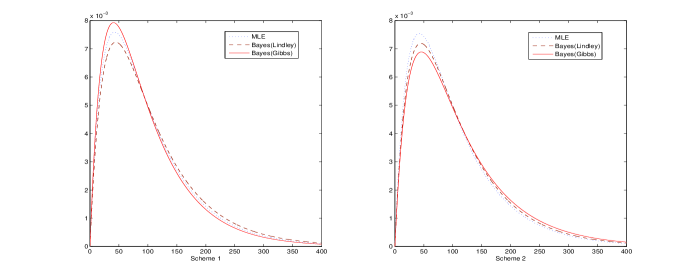
Figure 1: Estimated density functions with informative priors for scheme 1(left) and scheme 2(right).

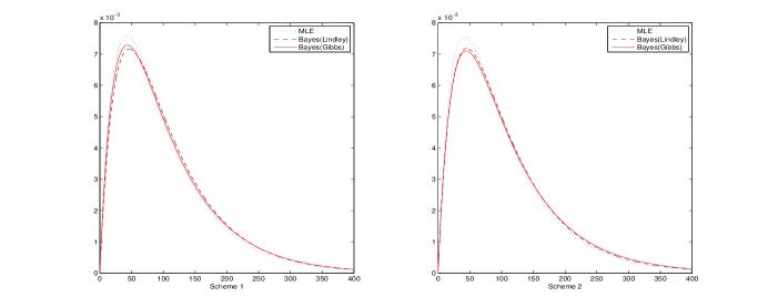
Figure 2: Estimated density functions with non-informative priors for scheme 1(left) and scheme 2(right).

Comparing the two schemes with informative and non-informative priors, it is observed that for scheme 1, estimators have smaller standard errors than scheme 2, as expected. Also it is clear that the Bayes estimators depend on the hyper parameters. Because the HPD confidence intervals based on informative priors are slightly smaller than corresponding length of HPD confidence intervals based on non-informative priors, therefore the prior informative should be used if they are available.

7 Conclusion

In this article, we have studied the classical and Bayes inference procedure for the Type-II hybrid censored $\mbox{WE}(\alpha,\lambda)$ distribution. We provide the maximum likelihood estimators and it is observed that the maximum likelihood estimators of the unknown parameters can not be obtained in the closed form and we suggest the EM algorithm to compute them. we also earn the Bayes estimators of the unknown parameters and show that they can not be obtained in explicit forms, and we have proposed two approximation methods to earn them. We have compared the performance of the different methods by Monte Carlo simulations, and it is observed that the performance of quite satisfactory.

Appendix A

Theorem 7.1

Given $X_{(1)}=x_{(1)},\cdots,X_{(r)}=x_{(r)}$, the conditional distribution of $Z_{i}$ for $i=1,\cdots,n-r$ is

$$f_{Z|X}(z_{i}|X_{(1)}=x_{(1)},\cdots,X_{(i)}=x_{(i)})=f_{Z|X}(z_{i}|X_{(i)}=x_{(i)})=\frac{f_{WE}(z_{i})}{1-F_{WE}(x_{i})}$$

where

$$f_{WE}(x)=\frac{\alpha+1}{\alpha^{2}}\beta e^{-\frac{\beta}{\alpha}x}(1-e^{-\beta x})$$

and

$$F_{WE}(x)=1-\frac{1}{\alpha}e^{-\frac{\beta}{\alpha}x}[\alpha+1-e^{-\beta x}]$$

Proof 7.1

The proof can be obtained similarly as in Ng et al. (2002).

Note that using Theorem 7, we can write

$$\begin{array}[]{c}A(c;\alpha,\beta)=E[Z_{i}|Z_{i}>c]=\int_{c}^{\infty}\frac{\alpha+1}{\alpha}\frac{\beta}{K}xe^{-\frac{\beta}{\alpha}x}(1-e^{-\beta x})dx\;\;\;\;\left(K=e^{-\frac{\beta}{\alpha}c}(\alpha+1-e^{-\beta c})\right)\\ \\ \hskip 72.26999pt=\frac{(\alpha+1)\alpha}{K\beta}\int_{\frac{\beta}{\alpha}c}^{\infty}ue^{-u}du-\frac{\alpha}{K\beta(\alpha+1)}\int_{\frac{\beta(\alpha+1)}{\alpha}c}^{\infty}ve^{-v}dv\;\;\;\left(put\;\;u=\frac{\beta}{\alpha}x\;\;\&\;\;v=\frac{\beta(\alpha+1)}{\alpha}x\right)\\ \\ =\frac{(\alpha+1)\alpha}{K\beta}(-e^{-u})(u+1)]_{\frac{\beta}{\alpha}c}^{\infty}-\frac{\alpha}{K\beta(\alpha+1)}(-e^{-v})(v+1)]_{\frac{\beta(\alpha+1)}{\alpha}c}^{\infty}\\ \\ =\frac{(\alpha+1)\alpha}{K\beta}(\frac{\beta}{\alpha}c+1)e^{-\frac{\beta}{\alpha}c}-\frac{\alpha}{K\beta(\alpha+1)}(\frac{\beta(\alpha+1)}{\alpha}c+1)e^{-\frac{\beta(\alpha+1)}{\alpha}c}\\ \\ =\frac{\alpha e^{-\frac{\beta}{\alpha}c}}{K\beta}\left[(\alpha+1)(\frac{\beta}{\alpha}c+1)-\frac{e^{-\beta c}}{\alpha+1}(\frac{\beta(\alpha+1)c}{\alpha}+1)\right]\\ \\ =\frac{e^{-\frac{\beta}{\alpha}c}}{K\beta}\left[(\alpha+1)(\beta c+\alpha)-\frac{e^{-\beta c}}{\alpha+1}\left(\beta(\alpha+1)c+\alpha\right)\right]\\ \\ \displaystyle=\frac{(\alpha+1)(\beta c+\alpha)-\frac{e^{-\beta c}(\beta c(\alpha+1)+\alpha)}{\alpha+1}}{\beta(\alpha+1-e^{-\frac{\beta}{\alpha}c})}\end{array}$$

and about $B(c;\alpha,\beta)$, we have:

$$B(c;\alpha,\beta)=E[\ln(1-e^{-\beta Z_{i}})|Z_{i}>c]=\int_{c}^{\infty}\frac{\alpha+1}{\alpha}\frac{\beta}{K}\ln(1-e^{-\beta x})e^{-\frac{\beta}{\alpha}x}(1-e^{-\beta x})dx$$

$$=-\frac{\alpha+1}{\alpha K}\int_{1-e^{-\beta c}}^{1}u(1-u)^{\frac{1}{\alpha}-1}\ln(u)$$

$$=\frac{\alpha+1}{\alpha K}\left[\frac{1}{18}(1-e^{-\beta c})^{3}(-\frac{1}{\alpha}+1)\mbox{hypergeom}_{3,2}([3,3,-\frac{1}{\alpha}+2],[4,4],1-e^{-\beta c})\right.$$

$$+\left(-\frac{1}{4}\mbox{hypergeom}_{2,1}([2,-\frac{1}{\alpha}+1],[3],1-e^{-\beta c})\right.$$

$$\left.+\frac{1}{2}\ln(x)\mbox{hypergeom}_{2,1}([2,-\frac{1}{\alpha}+1],[3],1-e^{-\beta c})\right)(1-e^{-\beta c})^{2}$$

$$-\frac{1}{18}(-\frac{1}{\alpha}+1)\mbox{hypergeom}_{3,2}([3,3,-\frac{1}{\alpha}+2],[4,4],1)$$

$$\left.+\frac{1}{4}\mbox{hypergeom}_{2,1}([2,-\frac{1}{\alpha}+1],[3],1)\right]$$

where hypergeom(.) is Generalized hypergeometric function. This function is also known as Barnes’s extended hypergeometric function. The definition of $F_{p,q}(\mathbf{n},\mathbf{d},\xi)$ is:

$$F_{p,q}(\mathbf{n},\mathbf{d},\xi)=\sum_{k=0}^{\infty}\frac{\lambda^{k}\Pi_{i=1}^{p}\Gamma(n_{i}+k)\Gamma^{-1}(n_{i})}{\Gamma(k+1)\Pi_{i=1}^{q}\Gamma(d_{i}+k)\Gamma^{-1}(d_{i})},$$

where $\mathbf{n}=[n_{1},\cdots,n_{p}]$, $p$ is the number of operands of $\mathbf{n}$, $\mathbf{d}=[d_{1},\cdots,d_{q}]$ and $q$ is the number of operands of $\mathbf{d}$. Generalized hypergeometric function is quickly evaluated and readily available in standard software such as Maple.

Appendix B

The conditional density of $\beta$ given $\alpha$ and $\b{x}$ is

$$\pi(\beta|\alpha,\b{x})\propto\beta^{w_{2}+r-1}e^{-\beta\left(w_{1}+\frac{\beta}{\alpha}\sum_{i=1}^{r}x_{i}+c(n-r)\right)}(\alpha+1-e^{-\beta c})^{n-r}\Pi_{i=1}^{r}(1-e^{-\beta x_{i}}).$$

This function is log-concave because we have

$$\frac{\partial^{2}\log(\pi(\beta|\alpha,\b{x}))}{\partial\beta^{2}}=-\frac{w_{2}+r-1}{\beta^{2}}-\frac{(n-r)c^{2}e^{-\beta c}(\alpha+1)}{(\alpha+1-e^{-\beta c})^{2}}-\sum_{i=1}^{r}\frac{x_{i}^{2}e^{-\beta x_{i}}}{(1-e^{-\beta x_{i}})^{2}}<0.$$

Therefore, the result follows.
 

Appendix C

The conditional distribution of $\alpha$ given $\beta$ and $\b{x}$ is

$$\pi(\alpha|\beta,\b{x})\propto\alpha^{w_{4}-n-r-1}(\alpha+1)^{r}e^{-\alpha w_{3}}e^{-\frac{\beta}{\alpha}(\sum_{i=1}^{r}x_{i}+c(n-r))}(\alpha+1-e^{-\beta c})^{n-r}.$$

In this function, we have $\pi(\infty|\beta,\b{x})\rightarrow\pi(0|\beta,\b{x})=0$ and $\pi(\alpha|\beta,\b{x})\geq 0~{}~{}\forall\alpha$, now it is enough that prove $\pi(\alpha|\beta,\b{x})$ is bounded. With simple calculation we see that $\forall\alpha$ this function is less than the gamma function and the gamma function is a bounded function, so this function is bounded. Therefore $\pi(\alpha|\beta,\b{x})$ has a finite maximum point.

References

• [1] Banerjee.A, Kundu.D (2008) Inference based on Type-II hybrid censored data from a Weibull distribution, IEEE Trans. Reliab., 57,Β  369-378.
• [2] Bjerkedal.T (1960) Acquisition of resistance in guinea pigs infected with different doses of virulent tubercle bacilli, Amer. J. Hyg., 72,Β  130-148.
• [3] Chen.S, Bhattacharya.G.K (1988) Exact confidence bounds for an exponential parameter under hybrid censoring, Comm. Statist. Theor. Meth., 17,Β  1857-1870.
• [4] Chen.M.H, Shao.Q.M (1999) Monte Carlo estimation of Bayesian Credible and HPD intervals, J. Comput. Graph. Statist., 8,Β  69-92.
• [5] Childs.A, Chandrasekhar.B, Balakrishnan.N, Kundu.D (2003) Exact likelihood inference based on Type-I and Type-II hybrid censored samples from the exponential distribution,Ann. Instit. Statist. Math., 55,Β  319-330.
• [6] Dempster.A.P, Laird.N.M, Rubin.D.B, (1977) Maximum likelihood from incomplete data via the EM algorithm (with discussion), J. Roy. Statist. Soc., Ser., 39,Β  1-38.
• [7] Devroye.L (1984) A simple algorithm for generating random variates with a log-concave density, Computing., 33,Β  247-257.
• [8] Draper.N, Guttman.I (1987) Bayesian analysis of hybrid life tests with exponential failure times, Ann. Inst. Statist. Math., 39,Β  219-225.
• [9] Dube.S, Pradhan.B, Kundu.D (2011) Parameter estimation of the hybrid censored log-normal distribution, J. Statist. Comput. Simul., 81,Β  275-287.
• [10] Ebrahimi.N (1992) Prediction intervals for future failures in exponential distribution under hybrid censoring, IEEE Trans. Reliab., 41,Β  127-132.
• [11] Ebrahimi.N (1990) Estimating the parameter of an exponential distribution from hybrid life test,J. Statist. Plann. Inference., 23,Β  255-261.
• [12] Epstein.B (1954) Truncated life tests in the exponential case, Ann. Math. Statist., 25,Β  555-564.
• [13] Fairbanks.K, Madson.R, Dykstra.R (1982) A confidence interval for an exponential parameter from a hybrid life test, J. Amer. Statist. Assoc., 77,Β  137-140.
• [14] Geman.S, Geman.A (1984) Stochastic relaxation, Gibbs distributions and the Bayesian restoration of images, IEEE Trans. Pattern Anal. Mach. Intell., 6,Β  721-740.
• [15] Gupta.R.D, Kundu.D (2009) A new class of weighted exponential distributions, J. Statistics., 43,Β  621-634.
• [16] Gupta.R.D, Kundu.D (2001) Exponentiated exponential family; an alternative to Gamma and Weibull, Biometr. J., 33,Β  117-130.
• [17] Gupta.R.D, Kundu.D (1998) Hybrid censoring schemes with exponential failure distribution, Commun. Statist. Theor. Meth., 27,Β  3065-3083.
• [18] Jeong.H.S, Park.J.I, Yum.B.J (1996) Development of (r,T) hybrid sampling plans for exponential lifetime distributions, J. Appl. Statist., 23,Β  601-607.
• [19] Kundu.D (2007) On hybrid censored Weibull distribution, J. Statist. Plann. Inference., 137,Β  2127-2142.
• [20] Kundu.D, Pradhan.B (2009) Estimating the parameters of the generalized exponential distribution in presence of hybrid censoring, Comm. Statist. Theor. Meth., 38,Β  2030-2041.
• [21] Lindley.D.V (1980) Approximate Bayesian methods, Trabajos de Estadistica., 31,Β  223-237.
• [22] Louis.T.A (1982). Finding the observed information matrix using the EM algorithm, J. Roy. Statist. Soc. Ser., 44,Β  226-233.
• [23] McLachlan.G.J, Krishnan.T (1997) The EM algorithm and extension, Wiley, New York.
• [24] MIL-STD-781-C (1977) Reliability Design Qualifications and Production Acceptance Test, Exponential Distribution, em US Government Printing Office, Washington, DC.
• [25] Zogbiy.A.M, Boasbasb.b (1998) The bootstrap and its application in signal processing, IEEE Signal Process. Magaz., 15,Β  56-76.