Perturbation of the Eigenvectors of the Graph Laplacian:
Application to Image Denoising
Abstract
The original contributions of this paper are twofold: a new understanding of the influence of noise on the eigenvectors of the graph Laplacian of a set of image patches, and an algorithm to estimate a denoised set of patches from a noisy image. The algorithm relies on the following two observations: (1) the low-index eigenvectors of the diffusion, or graph Laplacian, operators are very robust to random perturbations of the weights and random changes in the connections of the patch-graph; and (2) patches extracted from smooth regions of the image are organized along smooth low-dimensional structures in the patch-set, and therefore can be reconstructed with few eigenvectors. Experiments demonstrate that our denoising algorithm outperforms the denoising gold-standards.
keywords:
graph Laplacian , eigenvector perturbation , image patch , image denoisingurl]http://ecee.colorado.edu/ fmeyer
1 Introduction
1.1 Problem statement and motivation
The first goal of this work is to study experimentally the perturbation of the eigenvectors of the graph Laplacian constructed from a set of image patches. The second goal of the paper is to devise a novel method to jointly denoise an image and estimate the eigenvectors of the patch-graph of the clean image.
Recent work in computer vision and image processing indicates that the elusive quest for the “universal” transform has been replaced by a fresh new perspective. Indeed, researchers have recently proposed to represent images as “collage” of small patches. The patches can be shaped into square blocks [1] or into optimized contours that mimic the parts of a jigsaw puzzle [2]. These patch-based appearance models are generative statistical models that can be learned from images, and are then used to represent images. All the patch-based methods [e.g., 3, 4, 5, 6, 7, 8, 9, 10, and references therein] take advantage of the following fact: the dataset of patches, whether it is aggregated from a single image, or a library of images, is a smooth set. A consequence of this observation is that the eigenvectors of the graph Laplacian [11, 12] provide a natural basis to expand smooth functions defined on the set of patches. The image intensity – seen as a function on the patch-set – is obviously a smooth function. As a result, the eigenvectors of the graph Laplacian yield an efficient (measured in terms of sparsity, for instance) representation of the original image from which the patch-set is computed.
In practice, images are often corrupted by noise, and the eigenvectors are to be computed from a graph of noisy patches. The problem becomes: what is the effect of the noise on the perturbation of the eigenvectors? Theoretical results [13] provide upper bounds on the angle between the original and the perturbed eigenspaces. Unfortunately, as noted by Yan et al. [14], in the context of the perturbation of the first non trivial eigenvector of the graph Laplacian, these bounds usually overestimate the actual perturbation. In addition, the bounds depend on the separation of the eigenvalues, a quantity that is difficult to predict for image patches. Finally, bounds on the angle between invariant subspaces cannot be readily translated in terms of the effect of the perturbations on the geometric features encoded by the eigenvectors, or the ability of the perturbed eigenvectors to approximate the original image.
1.2 Outline of our approach and results
The original contributions of this paper are twofold: a new understanding of the influence of noise on the eigenvectors of the graph Laplacian and a new method to denoise image patches.
Our approach relies on a series of experiments aimed at understanding the effect of noise on the perturbations of the eigenvectors of the patch-graph. In particular, we show that the low order eigenvectors of the graph Laplacian are robust to random variations in the geometry of the graph and in the edge weights. These results are connected to similar results in spectral geometry quantifying the perturbations of the eigenfunctions of the Laplace-Beltrami operator as a function of changes in the metric of the manifold [15, 16]. Equipped with this experimental understanding of the robustness of the low index eigenvectors of the graph Laplacian, we propose an iterative procedure to jointly estimate the eigenvectors and the original image. We evaluate our novel approach with numerous experiments on a variety of images, and we compare our approach to some of the denoising gold-standards. Our approach systematically outperforms these algorithms.
2 The manifold of patches from a single image
We consider an image , of size . We extend the image by even symmetry when the pixel location becomes close to the border of the image. We first define the notion of a patch.
Definition 1
Let be a pixel with linear index . We extract an block, centered about ,
| (1) |
where, without loss of generality, we take to be an odd integer, and is the result of the Euclidean division of by 2. By concatenating the columns, we identify the matrix (1) with a vector in , and we define the patch by
| (2) |
As we collect all the patches, we form the patch-set in .
Definition 2
The patch-set is defined as the set of patches extracted from the image ,
| (3) |
Before we start exploring the effect of noise on the patch-set , let us pause for an instant and ask ourselves if is a smooth set. This question can be answered by ignoring for a moment the spatial sampling of the image that leads to pixelization. We imagine that the image intensity is a smooth function defined for . In this case, is clearly a two-dimensional smooth manifold. Even though the image is a function of a continuous argument , the patch is formed by collecting discrete samples on a lattice. Let be the horizontal, or vertical, lattice resolution. For any pair of translation indices , we consider the function that maps to the coordinate of the patch ,
| (4) |
This map is a smooth function from to , since is smooth. Therefore, each of the coordinates of is a smooth function of , and the map that assigns a pixel to its patch
| (5) |
is a smooth map from to . The non-discretized version of is thus a two-dimensional manifold in . We note that Grimes and Donoho [17] have argued that a set of binary images obtained by moving a black object on a white background forms a sub-manifold that is not differentiable. The lack of differentiability hinges on the fact that binary images can only have step edges that are not differentiable. In fact, smoothing the images allows one to recover the differentiability of the sub-manifold. In this work, we assume that the image has been blurred by the acquisition device, and therefore is a smooth function of .
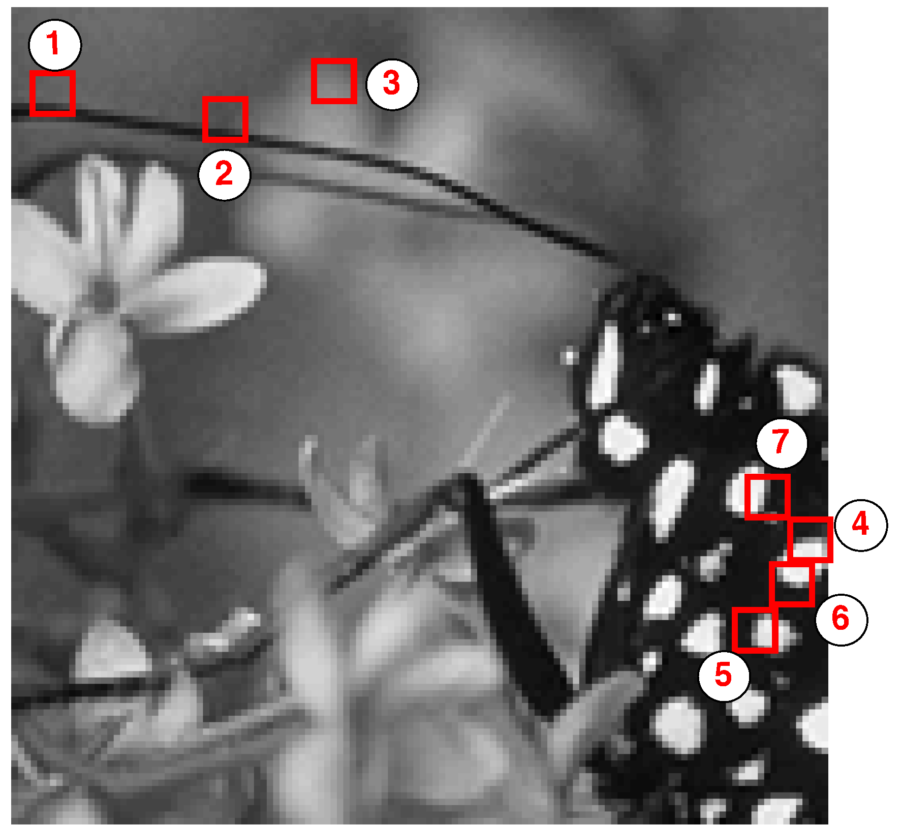
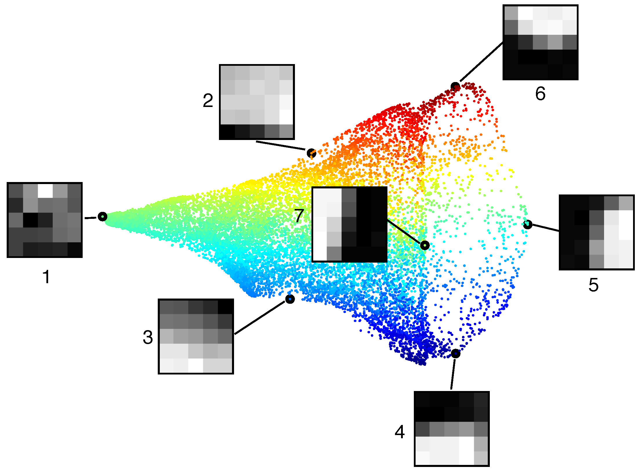
We provide an illustration of the patch submanifold in Fig. 1, where patches, extracted from the butterfly image (Fig. 1-left), form a smooth two-dimensional structure (Fig. 1-right). The cone-shaped surface encodes the content of the patches: as we move along the curve formed by the opening of the cone in Fig. 1-right, we explore patches (numbered 4, 5, 6 and 7) that contain high-contrast edges at different orientations. Each ruling (generator) of the cone is composed of all the patches that contain an edge with the same orientation. In effect, the orientation of the edge inside these patches is encoded by the position of the ruling on the opening curve. In addition, the white part of the patch is either always at the top, or always at the bottom (see e.g. and ). Finally, as we slide from the opening of the cone to its tip, the contrast across the edge decreases (see e.g. and ).
2.1 Denoising patch datasets
We now consider the problem central to this paper: denoising a patch dataset that lies close to a manifold . We review the two broad classes of approaches that have been proposed to solve
the more general problem of denoising a manifold-valued dataset:
-
1.
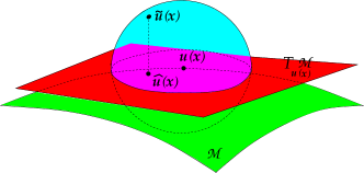
local methods that construct a local projector, which varies from point to point, and project the noisy measurements on a local estimate of the tangent plane (see Fig.2);
-
2.
global methods that denoise the entire dataset. Linear and nonlinear methods can be used to reconstruct an estimate of the clean manifold.
Local methods: denoising along the tangent plane. The concept of image patches is equivalent to the concept of time-delay coordinates in the context of the analysis of a dynamical system from the time series generated by an observable [18]. Several methods have been proposed to remove the noise from time-delay embedded data [e.g., 19, and references therein]. These methods rely on the estimation of a local coordinate system formed by the tangent plane to the manifold at (see Fig. 2). The tangent plane is computed from the singular value decomposition of a neighborhood of ; the first singular vectors provide a basis of the local tangent plane (see Fig. 2), while the remaining vectors capture the noise [e.g., 20, and references therein]. The noise, which is dimensional, is squashed by projecting the noisy data onto the tangent plane (see Fig. 2). Similar ideas have been proposed recently in the image processing literature. The BM3D algorithm [5] uses the local patches around a noisy reference patch to construct a local
orthonormal basis. A multiscale version of this concept was recently proposed to denoise curves [21]. Elad and co-workers proposed the k-SVD algorithm [22] that assembles multiple singular vectors, computed locally, in order to construct a global set of functions to represent an image.
Global methods: diffusion on the manifold. Instead of trying to approximate locally the manifold of patches by the tangent plane around each patch , global methods perform a comprehensive denoising on the entire manifold. The global denoising can be performed by applying a smoothing operator, defined by a kernel , to the noisy dataset and compute an estimate of from the noisy measurement ,
| (6) |
In practice, the Gaussian kernel is usually used, and the geodesic distance on the manifold is replaced by the Euclidean distance. The recent nonlocal means algorithm [3] can be recast as a discrete implementation of (6). Szlam et al. [6] have explicitly modeled the manifold of patches with a graph and implemented various diffusions on the graph. Singer et al. [23] provided a stochastic interpretation of nonlocal means as a diffusion process. Similar ideas were proposed in [24, 7, 5]. Gilboa and Osher [4] proposed a continuous version of this idea, and defined PDE-based flows that depend on local neighborhoods. Early on, the computer graphics community has been implementing discrete versions of (6) to smooth and denoise surface meshes [e.g., 25, and references therein]. Specifically, Taubin [25] proposed to implement (6) using the diffusion
| (7) |
where is a discrete approximation to the Laplacian operator defined on the mesh.
Global methods: from the diffusion operator to its eigenvectors. Instead of applying the diffusion kernel on the graph of patches, one can compute the eigenvectors of the graph Laplacian [11, 12], and use them to expand the corresponding diffusion kernel . The set of eigenvectors provides a spectral decomposition, similar to a global Fourier basis. If we keep only the first few eigenvectors of the expansion, the result is very similar to applying the diffusion operator for a long period of time (see section 4.2). In his seminal work, Taubin [25] proposed to use the eigenvectors of the graph Laplacian to denoise meshes. Szlam et al. [6] proposed to perform some nonlinear approximation using the eigenvectors of the graph Laplacian. Peyré [8] combined thresholding and regularization to remove noise from images.
In our problem, the diffusion operator needs to be estimated from the noisy data. Consequently, we expect that the eigenvectors of the noisy operator may be very different from the eigenvectors of the true operator . We intend to study the perturbation of the eigenvectors, and propose a method to denoise jointly the eigenvectors and the image.
3 The eigenvectors: a sparse code for images
3.1 The graph of patches: the patch-graph
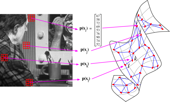
In this paper, we think about a patch, , in several different ways. Originally, is simply a block of an image. We also think about as a point in . Finally, we also regard as a vertex of a graph. Throughout this work, we will use these three perspectives. In order to study the discrete structure formed by the patch-set (3), we connect patches to their nearest neighbors, and construct a graph that we call the patch-graph (see Fig. 3).
Definition 3
The patch-graph, , is a weighted graph defined as follows.
-
1.
The vertices of are the patches .
-
2.
Each vertex is connected to its nearest neighbors using the metric
(8) -
3.
The weight along the edge is given by
(9)
The parameter controls the influence of the penalty term that measures the distance between the patches in the image domain. The distance is small if the image intensity is similar at and , , and and are not too far from one another . The parameter controls the scaling of the similarity between and when defining the edge weight . The particular form of the weight (9) ensures that drops rapidly to zero as becomes larger than . A very large (i.e. for all ) emphasizes the topology of the graph and promotes a very fast diffusion of the random walk through the patch-set. The other alternative: accentuates the difference between the patches, but is very sensitive to noise. We now define the weight matrix, which fully characterizes the patch-graph.
Definition 4
The weight matrix is the symmetric matrix with entries . The degree matrix is the diagonal matrix with entries .
Finally, we define the normalized Laplacian matrix.
Definition 5
The normalized Laplacian matrix is the symmetric matrix defined by
| (10) |
We note that the sign of the Laplacian is the opposite of the sign of the Laplacian on a manifold of dimension , defined by
| (11) |
where is the ball of radius centered around , and is the volume of the ball. Despite the fact that the discrete Laplacian has the wrong sign, it shares the structure of (11). Indeed, the entry of the vector is an average of the function defined on the graph, computed in a small neighborhood around the node . Similarly, computes the average of within a ball centered around . In both cases, the Laplacian measures the difference between and its local average.
The matrix is symmetric and positive definite, and has eigenvectors with corresponding eigenvalues . Each eigenvector is a vector with components, one for each vertex of the graph. Hence, we write
to emphasize the fact that we consider to be a function sampled on the vertices of . The eigenvectors form an orthonormal basis for functions defined on the graph, where the inner product on the graph is defined by
3.2 The eigenvectors encode the geometry of the image
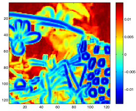
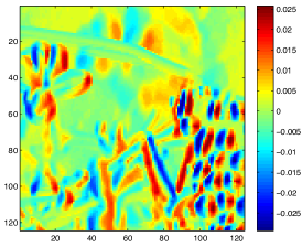
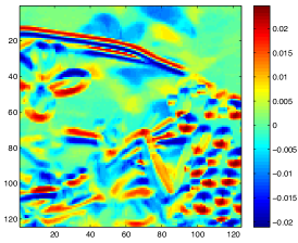
We can represent as an image: each pixel is color-coded according to the value of . Figure 4 shows the three vectors , and of the butterfly image (see Fig. 1-left). The first non trivial eigenvector encodes the gradient of the image intensity: takes large negative111We note that the sign of is arbitrary. values at pixels with large gradient (irrespective of its direction) and takes large positive values at pixels with small gradient. and clearly encode horizontal and vertical partial derivatives of . The frequency content of each eigenvector is loosely related to the eigenvalue . Unlike Fourier analysis, the basis functions have an
intrinsic scale given by the patch size. In this work we propose to use the eigenvectors as a basis to denoise the image intensity function .
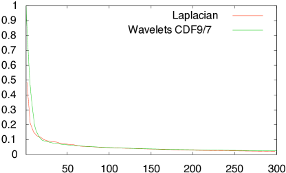
We conclude this section with experimental evidence that indicates that the image has a sparse representation in the basis . We will use this property in the next section to remove the noise from the image. Figure 5 displays the relative residual energy, , after reconstructing the clown image (Fig 3-left) using the first eigenvectors with the largest coordinates ,
For comparison purposes, the same quantity is computed using a wavelet decomposition. We see that the basis functions give rise to a very fast decay of the residual energy, even faster than with the 9/7 wavelet basis. We performed similar comparisons with several other images (not shown) that lead us to conclude that we could use this basis to denoise natural images.
4 Denoising
4.1 Denoising the patch-set using the noise-free eigenvectors
We describe in this section a denoising algorithm that constructs an estimate of the patch-set from the knowledge of the noisy image . The denoising of the patches is not performed locally on the patch-set, but rather relies on the global eigenvectors . This allows us to denoise the entire patch-set as a whole. We assume for the moment that we have access to the eigenvectors of the noise-free image. While this is clearly unrealistic, this allows us to explain the principle of the algorithm. In section 4.3 we study the effect of noise on the eigenvectors. Finally, in section 4.4, we describe a procedure to iteratively reconstruct the patch-set and the eigenvectors.
The original image has been corrupted by additive white Gaussian noise with variance , and we measure at every pixel the noisy image , given by
Let be the patch centered at associated with the noisy image , and let be the patch-set formed by the collection of noisy patches. We propose to construct an estimate of the clean patch-set from the noisy patch-set . Lastly, we will combine several denoised patches to reconstruct an estimate of the clean image at the pixel .
Let denote the coordinates of the patch . We define similarly, to be the coordinates of the patch . We make the following trivial observation: the coordinate is a real-valued function defined on the set of vertices
In order to denoise simultaneously all the patches, we denoise each coordinate function independently. This is achieved by expanding the function into the basis formed by the , and performing a nonlinear thresholding. The result is the denoised function , given by
| (12) |
where the function performs a nonlinear thresholding of the coefficients . In practice, we use a hard thresholding. After denoising all the coordinate functions , we have access to an estimate of the clean patch-set.
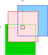
Because the patch-set has a maximum overlap (i.e. we have a patch for each pixel), there are patches that overlap (in the image domain) with the pixel (see Fig. 6). Let be the ball for the norm of radius pixels centered at ,
| (13) |
The patches that overlap with all have their center in (see Fig. 6). For each of the pixels , there exists an index in such that the coordinate of the patch corresponds to the pixel location . In other words, is an estimate of the image intensity at the location obtained from patch . We combine all these estimates and define the denoised image at pixel as the following weighted sum
| (14) |
where the exponential weight is given by
| (15) |
This choice of weights favors the patch centered at , and disregard exponentially fast the neighboring patches. We have also experimented with weights that discourage the mixing of patches with very different variances (results not shown).
Connection to translation-invariant denoising. We note that we can interpret the th coordinate function as the original image shifted by , where . For instance, if , then the two-dimensional shift is and if , the shift is . The reconstruction formula (14) can then be interpreted as a translation-invariant denoising procedure [26] of the form,
4.2 Geometric interpretation of the eigenvectors
We explain in this section the connection between our approach and denoising methods based on defining a diffusion process on the graph [6, 7]. The solution to the denoising problem is related to a diffusion process defined on the patch-set. Indeed, let us consider the image solution to the diffusion defined on the patch-graph (notice that we use the wrong sign for equation (7) as explained in section 3.1) defined by,
| (16) |
where the initial condition is provided by the noisy image ,
| (17) |
We consider the heat kernel formed by the matrix
| (18) |
and we write the solution to the diffusion as
| (19) |
We notice the similarity between the expansions (12) and (19). As becomes large, only a small number of terms in (19) will be non zero. The attenuation of is controlled by the size of the corresponding eigenvalue . This is in contrast to (12), where the coefficients used to reconstruct the denoised signal are chosen based on the magnitude of . The similarity between the two expansions allows us to understand what is the information encoded by each . In (19), each function is a stationary solution to the diffusion (16). The amplitude of this stationary solution decreases exponentially fast with time, but the geometry, encoded by remains unchanged. The eigenvectors therefore encode the geometric features present in the image: edges, texture, etc. as suggested by Fig. 4. Finally, we note that if the graph of patches is replaced with a regular lattice formed by the image sampling grid, and if each patch is reduced to a single pixel, then the diffusion (16) models one of the standard diffusion-based denoising algorithms [27].
4.3 Estimating the eigenvectors from the noisy images
We described in the previous section a denoising procedure that relies on the knowledge of the eigenvectors associated with the clean patch-set. Of course, if we had access to the clean patch-set, then we would have the clean image. While our approach appears to be circular, we claim that it is possible to bootstrap an estimate of the and iteratively improve this estimate. This approach relies on the stability of the low-frequency eigenspace of the graph Laplacian . In the next section we study experimentally the perturbation of the eigenvectors when a significant amount of noise is added to an image. We demonstrate that changes in the topology of the graph, and not changes in the weights, is the source of the perturbation of the . This result leads to an iterative method that recovers the clean eigenvectors that is described in section 4.4.
4.3.1 The eigenvectors of the perturbed Laplacian
Each patch of the clean image is corrupted by a multivariate Gaussian noise with diagonal covariance matrix, ,
| (20) |
The distance between any two noisy patches and is given by
| (21) |
with the corresponding expected value,
| (22) |
The weights associated with the noisy image are given by
| (23) |
While , the term may be greater than 1, thereby increasing . Overall, the presence of noise has two effects:
Let be the graph associated with the noisy patch-set . and have the same vertices, , and the same total number of edges (since both are based a nearest neighbor topology). The weight matrix is perturbed according to (23). We define and to be the weight and Laplacian matrices computed from the noisy image, respectively. We expect that the eigenvectors of will be different from the . As explained in the next section, the low-frequency eigenvectors remain stable, but the higher frequency eigenvectors rapidly degrade. As a result, cannot be used to reconstruct a clean image.
Theoretical results that provide upper bounds on the angle between an eigenspace of and the corresponding eigenspace of exist [13]. Unfortunately, as noted in [14], these bounds usually overestimate the actual perturbation of the eigenvectors. Furthermore, these results depend on the separation of the eigenvalues, a quantity that is difficult to predict in our problem. In fact the separation can be very small leading to very large bounds. Another limitations of the usual theoretical bounds is that the angle between two invariant subspaces cannot be readily translated in terms of the ability of the perturbed eigenvectors to approximate the original image using a small number of terms. We propose therefore to study experimentally the effect of the noise on the ability of to encode geometric information about the image. We employ standard methodology used in vision research. Specifically, let be the Fourier transform of , we study the energy distribution of using polar coordinates in the Fourier plane and we compute the average energy of over all orientation for a given radius .
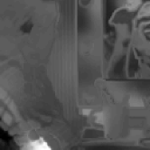
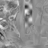
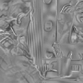
Our experiment was performed as follows. We add white Gaussian noise () to the clean clown image (see Fig. 7), and we compute the eigenvectors of the graph Laplacian. This image provides a good balance between texture and smooth regions; we performed similar experiences with other images, and obtained results that were quantitatively similar. The perturbed eigenvectors , , and are shown in the bottom row of Fig. 8. The eigenvectors of the clean image are shown in the top row of Fig. 8 for comparison purposes. We can make the following visual observations, which will be confirmed by a quantitative analysis in the next paragraph. For , the eigenvectors appear to be reasonably similar to the original eigenvectors . For ,
original noisy
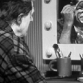
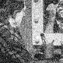
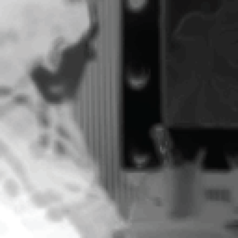
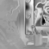
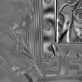
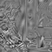
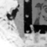
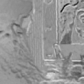
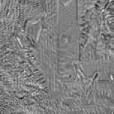
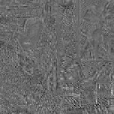
appear to mostly capture the random noise instead of the edges and texture present in the original image. For instance, the texture on the wallpaper and on the shirt of the clown, which is present in , is replaced by noise in (see Fig. 8).
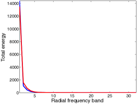
A quantitative analysis of the perturbation of the . We provide here a quantitative comparison between and . Our evaluation is based on the comparison between the energy distribution of the Fourier transforms and . Following a practice standard in vision research, we analyse as a function of the radial and angular frequencies, . Because we assume that the visual features (edges, textures, etc) can have any random orientation, we integrate over all possible orientation and compute the energy of within a thin ring ,
| (24) |
where the ring is defined by
The width of each ring () depends on the sampling frequency and the size of the image. In the experiments we use a total of rings, and for an image of size . In other words, there were two discrete frequencies within each ring . We do not study the perturbation of each eigenvector individually. Instead, we group the eigenvectors according to a dyadic scale of the index : the scale corresponds to the eigenvectors
This dyadic repacking of the eigenvectors was motivated by the experimental observation that the eigenvectors with the same dyadic scale had a similar Fourier transform. Finally, we compute at each scale the total energy contribution, integrated inside the ring , from the group of eigenvectors at that scale ,
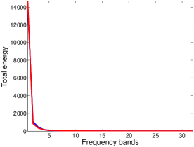
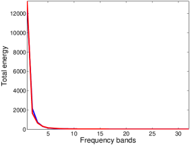
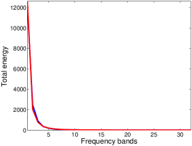
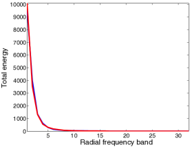
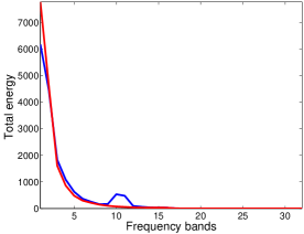
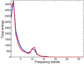
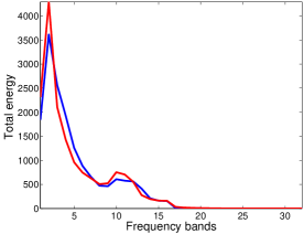
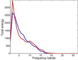
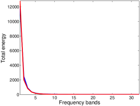
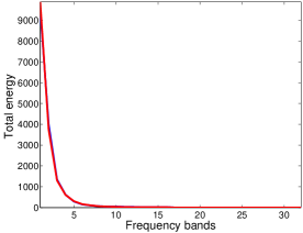
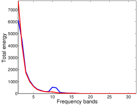
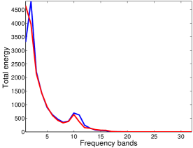
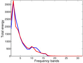
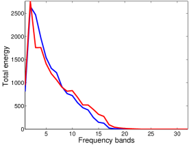
Figure 9 shows the energy distribution as a function of the radial frequency index , for the scales . For each plot, the -axis is the index of the ring , and therefore provides a quantization of the radial frequency. The -axis is the total energy contribution, measured inside the ring , from the group of eigenvectors at scale . We plot the energy of the perturbed eigenvectors (in blue), as well as the energy of the clean eigenvectors (in red).
For the first three scales , corresponding to , there is hardly any difference between the energy distribution of the clean and perturbed eigenvectors (see Fig. 9). Starting at scale , the energy of the perturbed eigenvectors becomes different from the energy of the clean eigenvectors: has a flatter distribution with more energy in the higher frequencies. The energy leak into the high radial frequencies is created by the noise and confirms the visual impression triggered by in Fig. 8. The high-index eigenvectors are trying to capture the noise present in the image . As the scale further increases, the departure of from becomes even more
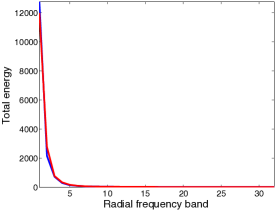
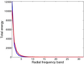
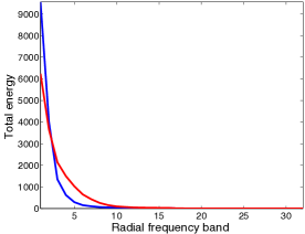
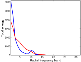
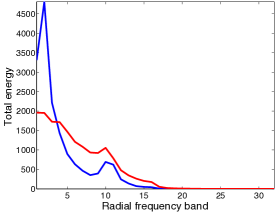
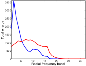
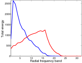 in blue
in red
dramatic. At scale , the radial energy distribution of the
eigenvectors is almost flat, indicating
that the have adapted to the noise. These eigenvectors are
obviously no longer suitable for denoising.
Which perturbation matters most: the topology of the graph, or the edge weights? As demonstrated in some recent studies [28, 29] topological changes of a graph (created by the addition or removal of edges) can significantly perturb the spectrum and the eigenvectors of the graph Laplacian. Inspired by these studies, we analyze the effect of the modifications of the topology of the graph on the eigenvectors .
Precisely, we verify experimentally the following result: if the non-zero entries in the matrix (9) are kept at the same locations (we keep the graph topology), and if we randomly perturb the weights according to (23), then the perturbed eigenvectors have almost the same energy distribution in the Fourier domain as the eigenvectors computed from the original weight matrix. In the previous paragraph we observed that random fluctuations of the weights combined with perturbations of the graph topology (caused by the random changes of the local distance, and the corresponding neighbors) significantly perturbed the eigenvectors of . Combining these two experiments, we conclude that the topology of the graph is the most important factor, since, if preserved, it guarantees the stability of the eigenvectors.
Let us now describe the experiment. We first build a patch-graph and a weight matrix based on the clean image. We now add a random realization of white Gaussian noise (), and compute the new weights according to (9), where the neighbors are now defined by the clean patch-graph. We then update all the non-zero entries of the matrix using the perturbed weights . This constitutes the perturbed matrix . We define accordingly.
We note that is not equal to the matrix , described in the previous paragraph. Indeed, the nonzero entries of correspond to the edges of the graph defined by the perturbed distance . In other words, only if and are neighbors, and and are also neighbors.
Let be the eigenvectors of the perturbed matrix . Figure 10 displays , , and . Despite the fact that the entries of the matrix have been perturbed by adding a large amount of noise to the image, the eigenvectors of the resulting matrix, , appear visually very similar to the original eigenvectors of . This observation is confirmed in Fig. 11, which shows the energy distribution as a function of the radial frequency for the two sets of eigenvectors: and . Remarkably, the distribution of energy of and , measured across the different radial frequencies in the Fourier plane, are very similar. The eigenvectors do not suffer from any significant perturbation despite very significant changes in the image patches.
This experimental result is related to similar properties in the context of spectral geometry. If we replace the graph by a manifold, and we consider that the weight matrix encodes the metric, then our experimental results are related to the more general phenomenon that involves the stability
 in blue
in red
of the eigenspaces of the Laplace-Beltrami operator when the metric on the manifold is perturbed continuously [15, 16]. In our case, the continuous changes of the metric correspond to changes in the weights .
In practice, we do not have access to , and therefore we cannot construct . However, the results of this section suggest that we should try and reconstruct an estimate of the graph topology, associated with . We combine the following two results to construct an estimate of .
-
1.
For most images, many of the entries of the weight matrix can be estimated from a lowpass version of the image. In other words,
where is a lowpass filter, and is a patch from the image . Indeed, unless we are studying patches that contain only high frequencies, most of the energy within the patch comes from the low frequencies.
-
2.
The eigenvectors from the very first scales, , are very stable even when a large amount of noise is added to the image. We can therefore use these eigenvectors to estimate a lowpass version of the original image.
The strategy for denoising is now clear. We compute the weight matrix and calculate the eigenvectors associated with the first scales . We use these eigenvectors to compute a coarse estimate of the lowpass part of the image, , using the procedure described in section 4.1. Because too few eigenvectors are used in this reconstruction, we add back a scaled version of the residual error (the difference between the noisy image and the denoised image ) to obtain the intermediate image defined by
| (25) |
where . at this point the image has been sufficiently denoised, and we construct a new graph. We note that we have experimented with a different procedure to compute the image , using standard lowpass filtering, or wavelet denoising. Using these alternate approaches, we obtain similar results, albeit of lower quality (results not shown).
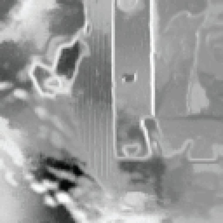
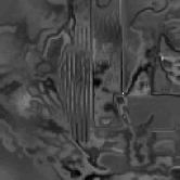
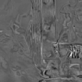
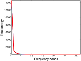
We finally compute the eigenvectors of associated to the image . Figure 12 displays the eigenvectors , , , and . These eigenvectors are visually similar to those

 in blue
in red
computed using the graph of the clean image (see Fig. 10). Figure 13 displays the distribution of the energy of the eigenvectors as a function of the radial frequency. Even at large scale and 7, the distribution of the energy of the across the radial frequency almost coincides with the distribution of the energy of the .
Szlam et al. [6] proposed a related approach to bootstrap a semi-supervised classifier: a new graph is constructed after one iteration of the classifier to improve the classification performance.
4.4 Iterative denoising
We propose an iterative procedure to denoise an image based on the results of the previous section. In practice we use two passes of denoising. The algorithm is described in Fig. 14. In the next section we study in details the two most important parameters of the algorithm: the patch sizes ( and ) and the numbers of eigenvectors ( and ) that are used during the two stages of the algorithm.
4.5 Optimization of the parameters of the algorithm
4.5.1 The patch size
While the eigenvectors provide a global basis on the patch-set, the patch size introduces a notion of local scale in the image. We notice visually that as the patch size increases, the eigenvectors become less crisp and more blurred. As explained in [23], [9] when the patch size is larger, patches are at a larger distance of one another in the patch-set. Consequently, a larger patch size prevents patches that are initially different from accidentally becoming neighbors after the image is corrupted by noise, since their mutual distance is relatively less perturbed by the noise. Because the eigenvectors are sensitive to the geometry of the patch-set, larger patches help minimize the perturbation of the eigenvectors. We note that, as patches become larger, the eigenvectors become more blurred, therefore requiring more eigenvectors to describe the texture. Finally, we need to be aware of the following practical limitation: if the patch size is large, and the image size is relatively small, then we have few patches to estimate the geometry of the patch-set; a problem aggravated by the fact that the patch-set lives in a large ambient space in that case.
We have compared the effect of the patch size on the quality of the denoised image after the first pass (stage 1) of the denoising algorithm (see Fig. 14). We define the signal to noise ratio
Algorithm: Two-pass denoising
-
Input: noisy image ;
-
number of nearest neighbors ; patch sizes ; scale parameters ;
-
number of eigenvectors ;
-
-
Output: the denoised image .
(SNR) by
| (26) |
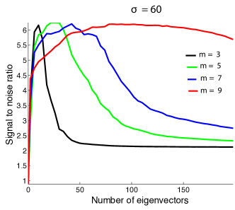
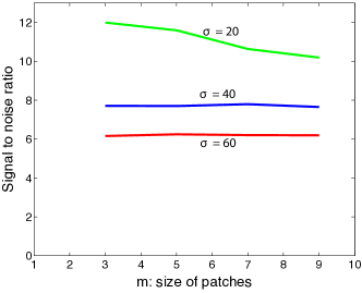
Figure 15 displays the signal-to-noise ratio as a function of the number of eigenvectors used to reconstruct , for different patch sizes , and at different noise levels ( and ). For low noise levels () the SNR is larger for smaller patches. For moderate noise levels, the maximum SNR achieved with different patch size is approximately the same (see Fig. 15 bottom-right). Nevertheless, the visual quality of the denoised images – at the same SNR – are quite
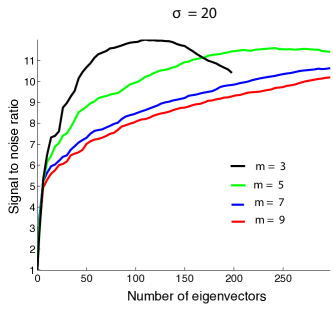
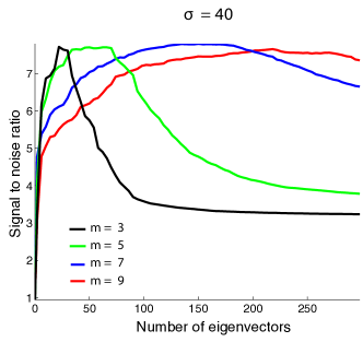

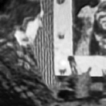

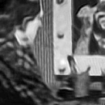
different. Figure 16 shows four denoised images () with very similar SNR, for and 9. With , the artifact caused by the noise can still be seen in the denoised image. However, with larger , the denoised image is much smoother, although some of the details in the original image are lost. The choice of the patch size is in general based on the noise level . In practice, we choose for , for , and for .
4.5.2 The number of eigenvectors
At both stages of the algorithm, the first eigenvectors are used to compute a denoised image. In general, the eigenvectors degrade faster as the variance of the noise level increases. We explain in the following why, using a very small number of eigenvectors, we can still reconstruct the structures of the patch-set that contain patches extracted from smooth regions of the image.
The local dimensionality of the patch-set. In this work we consider images that contain a mixture of smooth regions and texture. Therefore, we only need a very small number of eigenvectors to capture the patches extracted from smooth regions of the image. Indeed, as explained by Taylor and Meyer [9], patches extracted from smooth regions of the image align themselves along smooth low-dimensional structures. Indeed, for smooth patches, spatial proximity (in the image) implies proximity in . Conversely, patches that contain large gradients and texture are usually scattered across [9]. Other researchers have made similar experimental observations. For instance, Chandler and Field [30], Zontak and Irani [10] observed that patches can be classified into two classes according to their mutual distances. One class is composed of patches extracted from smooth regions, and the other class encompasses patches extracted from regions that contain texture, fast oscillation, large gradient, etc. These authors observe that “smooth patches” are at a small distance (in the patch-set) of one another, and are also at a close spatial distance (in pixels). They also note that proximity between “texture patches” is not dictated by spatial proximity (in pixels). Texture patches are scattered in because they are at a large distance of one another: Zontak and Irani [10] estimate that the distance to the nearest neighbor of a patch grows exponentially with the gradient within that patch. Finally, Taylor and Meyer [9] have shown that the local dimensionality of the patch-set is much lower around smooth patches, and much higher around texture patches.
Consequently, the smooth low-dimensional structures formed by the smooth patches can be accurately represented with a very small number of eigenvectors. Because low-index eigenvectors are very stable, we are able to reconstruct the smooth patches using the first few eigenvectors of . This partial reconstruction can then be used to estimate a new patch graph. The reconstruction
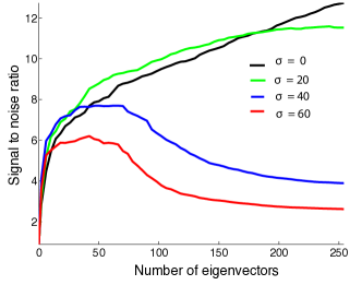
of the texture patches requires many more eigenvectors because that part of the patch-set has a much higher local dimensionality. Using the second graph, one can then compute more stable eigenvectors, and reconstruct the texture patches.
Figure 17 displays the SNR of after a one-stage reconstruction of the clown image as a function of the number of eigenvectors, for several noise levels. The patch size was , except for where it was . As we increase the number of eigenvectors , the SNR initially increases. Except at very low noise level (), the SNR decreases after it reaches its maximum. Indeed, at moderate and high noise levels, the high index eigenmodes adapt to the incoherent structure of the noise and become useless for the reconstruction. This is why we need a second pass in the reconstruction. Figure 17 can help us determine the numbers and of eigenvectors needed for the first and second denoising passes.
5 Experiments
We implemented the two-stage denoising algorithm (see Fig. 14) and evaluated its performance against several denoising gold-standards. For all experiments, we kept and eigenvectors during the first and second passes of the algorithm, respectively. The patch sizes for the first pass were for , and for , respectively. We used for all noise levels in the second pass of the algorithm.
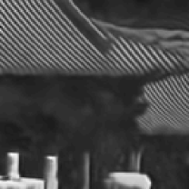
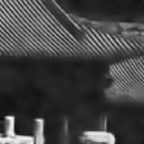
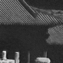
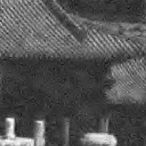
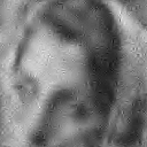
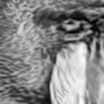
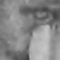
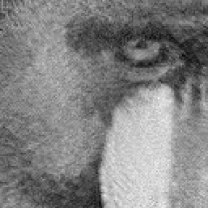
The evaluation was performed using five images that contain a mixture of smooth regions, periodic and aperiodic texture (see Fig. 18). White Gaussian noise was added to the images. We


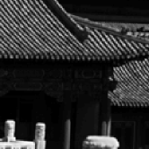
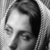
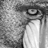


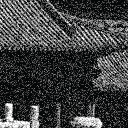
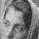
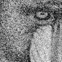
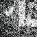
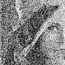
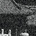
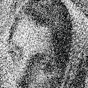
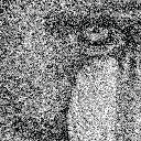
used two noise levels: moderate (Fig. 18 middle row), and high (Fig. 18 bottom row). We compared our approach to the following three denoising algorithms:
-
1.
translation invariant soft wavelet thresholding (TISWT) method [26]. We used the implementation provided by Wavelab (http://www-stat.stanford.edu/~wavelab/).
-
2.
nonlocal means [3]. We used the implementation provided by Jose Vicente Manjón Herrera and Antoni Buades (http://personales.upv.es/jmanjon/).
-
3.
k-SVD algorithm [22]. We used the implementation provided by Ron Rubinstein (http://www.cs.technion.ac.il/~ronrubin).
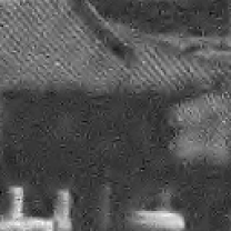
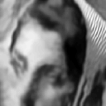
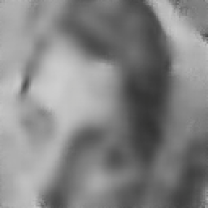
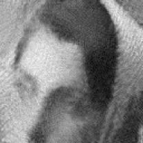
Table 1 displays the mean squared error between the reconstructed image and the original images,
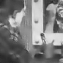
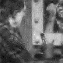
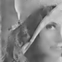
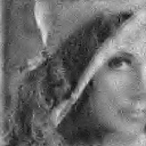
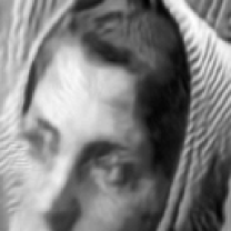
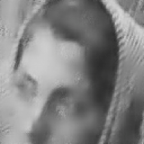
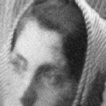
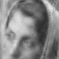
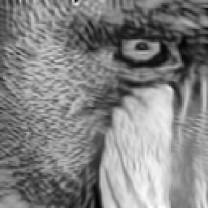
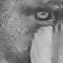
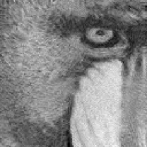
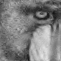
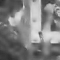
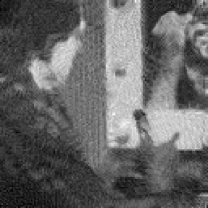
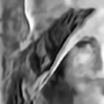
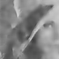
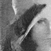
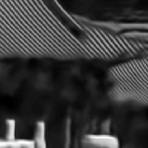
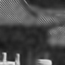
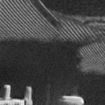
At all noise levels, and for all images our algorithm outperformed the other algorithms in terms of mean squared error. In terms of visual quality, the wavelet denoising yielded consistently the worst
noise level Laplacian k-SVD NL-means TISWT clown 40 216 261 252 359 60 354 509 447 585 lena 40 184 236 248 329 60 298 413 382 529 roof 40 196 318 221 486 60 310 542 395 767 barbara 40 116 160 168 241 60 191 300 290 436 mandrill 40 314 366 357 418 60 442 542 480 621
reconstruction. Missing wavelet coefficients are very noticeable, even at moderate noise level. K-SVD and nonlocal means yielded similar results. The nonlocal means estimate was always more noisy than the k-SVD estimate, which was often too smooth. In comparison, our approach could restore the smooth regions and the texture (see e.g. the mandrill image at and ), even at high noise level.
6 Discussion
We proposed a two-stage algorithm to estimate a denoised set of patches from a noisy image. The algorithm relies on the following two observations: (1) the low-index eigenvectors of the diffusion, or Laplacian, operators are very robust to random perturbations of the weights and random changes in the connections of the graph; and (2) patches extracted from smooth regions of the image are organized along smooth low-dimensional structures of the patch-set, and therefore can be reconstructed with few eigenvectors. Experiments demonstrate that our denoising algorithm outperforms the denoising gold-standards. This work raises several questions that we address in the following.
6.1 Fast computation of the eigenvectors
A key tenet of this work is our ability to compute the eigenvectors of the sparse matrix , which has size but with only non zero entries on each row. For the experiments we used the restarted Arnoldi method for sparse matrices implemented by the Matlab function eigs to solve the eigenvalue problem.
There are several options for further speeding up the computation of the eigenvectors. Saito [31] proposes to modify the eigenvalue problem, and compute the eigenvectors via the integral operator that commutes with the Laplacian. This approach leads to fast algorithms. The recent work of Kushnir et al. [32] indicates that multigrid methods yield an immediate improvement over Krylov subspace projection methods (e.g. Arnoldi’s method). Another appealing approach involves fast randomized methods [33]. We note that the application of these methods still necessitates the computation of the entire matrix . We believe that more efficient methods that randomly sample the patch-set should be developed. While the sampling density should clearly guarantee that short wavelength (high-index) eigenvectors are adequately sampled, we can probably estimate the low-index eigenvectors with a very coarse sampling. Similar ideas have been recently proposed for the reconstruction of manifolds [34].
6.2 Extension
This work opens the door to a new generation of image processing algorithms that use the eigenvectors of the graph Laplacian to filter the patch-set. We note that some of the most successful inpainting and super-resolution algorithms already operate locally on the patch-set [e.g., 35, and references therein]. These algorithms currently do not take advantage of the existence of global basis functions to represent the patch-set. Additional extensions include the construction of patch-sets from large collections of images. Lee and Mumford [36] demonstrated that high-contrast patches extracted from optical images were organized around 2-dimensional smooth () sub-manifold. Simple models of synthetic images were constructed in [8] and were shown to lie close to low-dimensional manifolds. We note that the set of all image patches includes the sub-manifold of patches constructed from a single image, which is the sub-manifold studied in this paper.
6.3 Open questions
This work provides experimental evidence of the stability of the low-indices eigenvectors of the Laplacian defined on a graph. Similar results exist in the literature in the context of the stability
Laplacian k-SVD NL-means TISWT




Laplacian k-SVD NL-means TISWT
Laplacian k-SVD NL-means TISWT



Laplacian k-SVD NL-means TISWT
of the eigenvectors of the Laplace-Beltrami operator when the domain is perturbed [37], or when the metric is perturbed [15, 16]. To the best of our knowledge, there appears to be little work on more precise analysis of the perturbation of the eigenspaces of the graph Laplacian. Yan et al. [14] acknowledge that standard bounds (e.g. [13]) overestimate the perturbations of the first eigenvector of the matrix .
Acknowledgments
FGM was partially supported by National Science Foundation Grants DMS 0941476, ECS 0501578, and DOE award DE-SCOO04096. This work benefited from fruitful discussions with Raphy Coifman, Peter Jones, and Arthur Szlam, during the 2009 IPAM Workshop on “Laplacian Eigenvalues and Eigenfunctions: Theory, Computation, Application”.
References
- Cheung et al. [2008] V. Cheung, B. Frey, N. Jojic, Video epitomes, International Journal of Computer Vision 76 (2008) 141–152.
- Kannan et al. [2007] A. Kannan, J. Winn, C. Rother, Clustering appearance and shape by learning jigsaws, Advances in Neural Information Processing Systems 19 (2007) 657.
- Buades et al. [2005] A. Buades, B. Coll, J. M. Morel, A review of image denoising algorithms, with a new one, Multiscale Modeling and Simulation 4 (2005) 490–530.
- Gilboa and Osher [2008] G. Gilboa, S. Osher, Nonlocal operators with applications to image processing, Multiscale Model. Simul. 7(3) (2008) 1005–1028.
- Dabov et al. [2009] K. Dabov, A. Foi, V. Katkovnik, K. Egiazarian, BM3D image denoising with shape-adaptive principal component analysis, in: Workshop on signal processing with adaptive sparse structured representations, 2009, pp. 1–6.
- Szlam et al. [2008] A. Szlam, M. Maggioni, R. Coifman, Regularization on graphs with function-adapted diffsion processes, Journal of Machine Learning Research 9 (2008) 1711–1739.
- Bougleux et al. [2009] S. Bougleux, A. Elmoataz, M. Melkemi, Local and nonlocal discrete regularization on weighted graphs for image and mesh processing, Intern. J. Comput. Vis. 84 (2009) 220–236.
- Peyré [2008] G. Peyré, Image processing with non-local spectral bases, SIAM Journal on Multiscale Modeling and Simulation 7 (2008) 703–730.
- Taylor and Meyer [2011] K. Taylor, F. Meyer, A random walk on image patches, 2011. Submitted to SIAM Journal on Imaging Sciences; available from http://arxiv.org/abs/1107.0414.
- Zontak and Irani [2011] M. Zontak, M. Irani, Internal statistics of a single natural image, in: IEEE Conference on Computer Vision and Pattern Recognition, 2011, pp. 977 –984.
- Belkin and Niyogi [2003] M. Belkin, P. Niyogi, Laplacian eigenmaps for dimensionality reduction and data representation, Neural Comput. 15 (2003) 1373–1396.
- Coifman and Maggioni [2006] R. R. Coifman, M. Maggioni, Diffusion wavelets, Appl. Comput. Harmon. A. 21 (2006) 53 – 94.
- Stewart and Sun [1990] G. Stewart, J. Sun, Matrix perturbation theory. computer science and scientific computing, Academic Press, Boston (1990).
- Yan et al. [2009] D. Yan, L. Huang, M. Jordan, Fast approximate spectral clustering, in: ACM SIGKDD International Conference on Knowledge Discovery and Data Mining, 2009, pp. 907–916.
- Barbatis [1996] G. Barbatis, Stability of weighted Laplace-Beltrami operators under -perturbation of the Riemannian metric, Journal d’Analyse Mathématique 68 (1996) 253–276.
- Davies [1990] E. Davies, Spectral properties of compact manifolds and changes of metric, American Journal of Mathematics (1990) 15–39.
- Grimes and Donoho [2005] C. Grimes, D. Donoho, Image manifolds which are isometric to euclidean space, Jal of Math. Imag. and Vision 23 (2005) 5–24.
- Gilmore [1998] R. Gilmore, Topological analysis of chaotic dynamical systems, Rev. Modern Phys. 70 (1998) 1455–1529.
- Kostelich and Schreiber [1993] E. Kostelich, T. Schreiber, Noise reduction in chaotic time-series data: a survey of common methods, Phys. Rev. E 48 (1993) 1752–1763.
- Kaslovsky and Meyer [2011] D. Kaslovsky, F. Meyer, Optimal tangent plane recovery from noisy manifold samples, 2011. Submitted to The Annals of Statistics available from http://http://arxiv.org/abs/1111.4601.
- Feiszli and Jones [2011] M. Feiszli, P. Jones, Curve denoising by multiscale singularity detection and geometric shrinkage, Applied and Computational Harmonic Analysis (2011).
- Aharon et al. [2006] M. Aharon, M. Elad, A. Bruckstein, On the uniqueness of overcomplete dictionaries, and a practical way to retrieve them, Linear Algebra and its Applications 416 (2006) 48–67.
- Singer et al. [2009] A. Singer, Y. Shkolnisky, B. Nadler, Diffusion Interpretation of Nonlocal Neighborhood Filters for Signal Denoising, SIAM Journal of Imaging Sciences 2 (2009) 118–139.
- Hein and Maier [2007] M. Hein, M. Maier, Manifold denoising, in: B. Schölkopf, J. Platt, T. Hoffman (Eds.), Advances in Neural Information Processing Systems 19, MIT Press, 2007, pp. 561–568.
- Taubin [1995] G. Taubin, A signal processing approach to fair surface design, in: SIGGRAPH ’95: Proceedings of the 22nd annual conference on Computer graphics and interactive techniques, ACM, 1995, pp. 351–358.
- Coifman and Donoho [1995] R. Coifman, D. Donoho, Translation-invariant denoising, in: A. Antoniadis, G. Oppenheim (Eds.), Wavelets and Statistics, Springer-Verlag, 1995, pp. 125–150.
- Morel and Solimini [1995] J. Morel, S. Solimini, Variational Methods for Image Segmentation, Birkhäuser, Boston, 1995.
- McGraw and Menzinger [2008] P. McGraw, M. Menzinger, Laplacian spectra as a diagnostic tool for network structure and dynamics, Physical Review E 77 (2008) 031102.
- Milanese et al. [2010] A. Milanese, J. Sun, T. Nishikawa, Approximating spectral impact of structural perturbations in large networks, Physical Review E 81 (2010) 046112.
- Chandler and Field [2007] D. Chandler, D. Field, Estimates of the information content and dimensionality of natural scenes from proximity distributions, JOSA A 24 (2007) 922–941.
- Saito [2008] N. Saito, Data analysis and representation on a general domain using eigenfunctions of laplacian, Appl. Comput. Harmon. A. 25 (2008) 68–97.
- Kushnir et al. [2010] D. Kushnir, M. Galun, A. Brandt, Efficient multilevel eigensolvers with applications to data analysis tasks, IEEE Trans. on Pattern Anal. and Machine Intell. 32 (2010) 1377–1391.
- Halko et al. [2011] N. Halko, P. Martinsson, J. Tropp, Finding structure with randomness: Probabilistic algorithms for constructing approximate matrix decompositions., SIAM Review 53(2) (2011) 217–288.
- Baraniuk and Wakin [2009] R. Baraniuk, M. Wakin, Random projections of smooth manifolds, Foundations of Computational Mathematics 9 (2009) 51–77.
- Criminisi et al. [2004] A. Criminisi, P. Pérez, K. Toyama, Region filling and object removal by exemplar-based image inpainting, Image Processing, IEEE Transactions on 13 (2004) 1200–1212.
- Lee et al. [2003] A. Lee, K. Pedersen, D. Mumford, The nonlinear statistics of high-contrast patches in natural images, International Journal of Computer Vision 54 (2003) 83–103.
- Barbatis et al. [2010] G. Barbatis, V. Burenkov, P. Lamberti, Stability estimates for resolvents, eigenvalues, and eigenfunctions of elliptic operators on variable domains, in: Around the Research of Vladimir Maz’ya, II, Springer, 2010, pp. 23–60.