Chaos and Nonlinear Dynamics in a Quantum Artificial Economy

Abstract

Chaos and nonlinear economic dynamics are addressed for a quantum coupled map lattice model of an artificial economy, with quantized supply and demand equilibrium conditions. The measure theoretic properties and the patterns that emerge in both the economic business volume dynamics’ diagrams as well as in the quantum mean field averages are addressed and conclusions are drawn in regards to the application of quantum chaos theory to address signatures of chaotic dynamics in relevant discrete economic state variables.

E-mail: cgoncalves@iscsp.utl.pt

1 Introduction

Economic systems, worked from complex systems’ science and nonlinear dynamics [1, 4, 5, 6, 7, 18, 21], can be approached in terms of either continuous state or discrete state systems [27]. Discrete state systems’ modelling tools, such as cellular automata, address the systems’ state transition in terms of discrete state maps, while continuous state systems are addressed in terms of continuous state equations of motion, either in discrete time (dynamical maps) or continuous time (differential equations).

The fact that, in most industries, the transactioned quantities are discrete, might seem to render support to discrete state rather than continuous state approaches. The present work’s proposal is that there may be a bridge between the two approaches, such that, through the application of the mathematical formalism of quantum mechanics to repeated (iterated) business games, one is able to integrate continuous state nonlinear dynamical systems’ models with discrete states.

The resulting approach leads to an application of quantum chaos within mathematical economics. By quantum chaos it is understood here the quantum behavior of a dynamical system which on average is classically chaotic [2, 23]. Since, in this case, we are dealing with economic systems, we provide, in section 2., for a quantum game theoretical framework within which quantized behavior in economic equilibrium can be understood, including an economic-based interpretation of the ket vectors in terms of risk pricing and a quantum game equilibrium condition that leads to a coherent state solution.

In section 3., we integrate the approach of section 2. with an evolutionary game of an artificial economy, formalized in terms of a quantum coupled map lattice with chaotic dynamics in the quantum averages. The measure-theoretic properties of the resulting (quantum) dynamical system as well as major dynamical features are addressed.

In section 4., we conclude with a reflection, in light of section 3.’s results, on the application of quantum chaos to nonlinear mathematical economics.

2 Quantum Economics of Supply and Demand

Let us consider an economy comprised of a population of $N$ competing companies, such that, for each company, there are the following (local) linear supply and demand functions:

$$Q^{s}\left(p_{t}(i)\right)=s\left(p_{t}(i)-\bar{p}\right)$$ (1)

$$Q^{d}\left(p_{t}(i)\right)=d_{t}(i)-kp_{t}(i)$$ (2)

where $i$ indexes a company and $t$ indexes a given discrete transaction round for the economy, $\bar{p}$ is the economy-wide smallest price at which any company is willing to sell its supply, $k$ and $s$ are fixed and characteristic of the economy, while the autonomous demand $d_{t}(i)$ is company-specific and dynamic, such that equilibria change by displacements of the (entire) demand line.

Each transaction round has a finite fixed duration and all transactions are assumed to take place at the end of the round and obey the equilibrium condition:

$$Q^{d}\left(p_{t}(i)\right)=Q^{s}\left(p_{t}(i)\right)=Q_{t}(i)$$ (3)

where $Q_{t}(i)$ are the equilibrium quantities. Letting $\phi:=\frac{1}{k}+\frac{1}{s}$ and $\theta:=\frac{\bar{p}}{\phi}$, solving for the equilibrium price, we obtain:

$$Q_{t}(i)=\frac{d_{t}(i)}{\phi}+\theta$$ (4)

Now, assuming that the quantities bought and sold are discrete undividable units, we must have that $Q_{t}(i)$ can only assume discrete values, thus, to address such a discrete demand we must assume a quantization scheme such that we replace the dynamical variable $Q_{t}(i)$ by an operator $\hat{Q}(i)$ on the economy’s Hilbert space $\mathcal{H}_{Economy}$, which is assumed to be spanned by the basis $\left\{\left|n_{1},n_{2},...,n_{N}\right\rangle:n_{i}\in\mathbb{N}_{0},i=1,2,...,N\right\}$ and such that:

$$\hat{Q}(i)=\frac{\hat{d}(i)}{\phi}+\theta$$ (5)

$$\hat{d}(i)=\hat{a}(i)^{\dagger}\hat{a}(i)\phi$$ (6)

$$a^{\dagger}(i)\left|...,n_{i},...\right\rangle=\sqrt{n_{i}+1}\left|...,n_{i}+1,...\right\rangle$$ (7)

$$a(i)\left|...,n_{i},...\right\rangle=\sqrt{n_{i}}\left|...,n_{i}-1,...\right\rangle$$ (8)

$$\left[a(i),a^{\dagger}(j)\right]=\delta_{i,j}$$ (9)

$$a_{i}\left|...,n_{i}=0,...\right\rangle=0$$ (10)

thus, replacing Eq.(6) in Eq.(5), we obtain the operator for the equilibrium quantities:

$$\hat{Q}(i)=\hat{a}(i)^{\dagger}\hat{a}(i)+\theta$$ (11)

where $\hat{a}(i)^{\dagger}$ and $\hat{a}(i)$ are interpreted as quantity raising and lowering operators for the company $i$, which, from Eqs. (7) to (10), behave like bosonic creation and annihilation operators. The spectrum of each company’s quantities’ operator is, then, given by:

$$\hat{Q}(i)\left|...,n_{i},...\right\rangle=\left(n_{i}+\theta\right)\left|...,n_{i},...\right\rangle$$ (12)

where $\theta$ has to assume an integer value, since quantities are, by assumption, expressed in whole numbers. In this way, $\theta$ is the smallest equilibrium quantity that can be sold in the market for any given company’s supply.

We may now introduce the complete projector set onto the basis of the economy’s Hilbert space $\left\{\hat{P}_{\boldsymbol{n}}=\left|\boldsymbol{n}\right\rangle\left\langle\boldsymbol{n}\right|:\left|\boldsymbol{n}\right\rangle=\left|n_{1},n_{2},...,n_{N}\right\rangle;n_{i}\in\mathbb{N}_{0},i=1,2,...,N\right\}$, each such projector has the matrix form of a quantum Arrow-Debreu security [12], which pays one unit of numeraire in the corresponding equilibrium state and zero units in all the others, assuming this analogy, we can bring to the quantum game setting an economic interpretation that fully integrates the quantum formalism in the economic framework to which it is being applied.

Therefore, at each round of the game, the economy is assumed to be characterized by a normalized ket vector $\left|\Psi(t)\right\rangle\in\mathcal{H}_{Economy}$, such that:

$$\left|\Psi(t)\right\rangle=\frac{1}{\sqrt{B}}\sum_{\boldsymbol{n}}\psi\left(\boldsymbol{n},t\right)\left|\boldsymbol{n}\right\rangle$$ (13)

where the round $t$ amplitude $\psi(\boldsymbol{n},t)=\left\langle\boldsymbol{n}|\Psi(t)\right\rangle$ is interpreted as the beginning-of-round infimum selling price amplitude for the end-of-round risk exposure $\hat{P}_{\boldsymbol{n}}$, or upper prevision amplitude, while the conjugate amplitude $\psi(\boldsymbol{n},t)^{*}=\left\langle\Psi(t)|\boldsymbol{n}\right\rangle$ is the beginning-of-round supremum buying price amplitude for the end-of-round risk exposure $\hat{P}_{\boldsymbol{n}}$, or lower prevision amplitude, in this way, the price for risk is $\left\langle\boldsymbol{n}\left|\hat{P}_{\boldsymbol{n}}\right|\boldsymbol{n}\right\rangle=|\psi(\boldsymbol{n},t)|^{2}=\psi(\boldsymbol{n},t)^{*}\psi(\boldsymbol{n},t)$, this is a quantum Arrow-Debreu price or quantum state-contingent price [12]. From the normalization condition, we have $\sum_{\boldsymbol{n}}|\psi(\boldsymbol{n},t)|^{2}=B$, where $B$ is a discount factor for the duration of a game round.

In this way, $\frac{|\psi(\boldsymbol{n},t)|^{2}}{B}$ are the end of round Arrow-Debreu capitalized prices and, from the way in which they are calculated, can be stated to satisfy the following relation:

$$\underline{P}\left[\hat{P}_{\boldsymbol{n}}\right]=\frac{|\psi(\boldsymbol{n},t)|^{2}}{B}=\overline{P}\left[\hat{P}_{\boldsymbol{n}}\right]$$ (14)

where $\underline{P}\left[\hat{P}_{\boldsymbol{n}}\right]$ and $\overline{P}\left[\hat{P}_{\boldsymbol{n}}\right]$ are, respectively, the lower and upper previsions on the alternative $\hat{P}_{\boldsymbol{n}}$ [25], therefore, each $\hat{P}_{\boldsymbol{n}}$ can be stated to be priceable such that the infimum acceptable selling price (upper prevision) and the supremum acceptable buying price (lower prevision) for a transaction on a risk exposure to $\hat{P}_{\boldsymbol{n}}$ both coincide with $\frac{|\psi(\boldsymbol{n},t)|^{2}}{B}$. Thus, if a bet were made on the risk exposure $\hat{P}_{\boldsymbol{n}}$, then, its end-of-round fair price would be $\frac{|\psi(\boldsymbol{n},t)|^{2}}{B}$ synthesizing, simultaneously, a price and a likelihood.

While classical probabilities are pure numbers, a probability with classical additivity that comes from the coincidence between an upper and lower prevision can be expressed in monetary units, such that it expresses, in the pricing, a statement about the risk and, thus, the likelihood of an event, the fair price $\frac{|\psi(\boldsymbol{n},t)|^{2}}{B}$ is, therefore, an expression on an exposure to a risk situation which reflects a likelihood systemic evaluation, that is, the fair pricing of risk must reflect the the risky event’s likelihood, and, therefore, we are dealing with a risk cognition as a systemic cognitive synthesis about risk, enacted by a complex adaptive system (in the present case, it is the system of companies).

This pricing is a systemic cognitive synthesis, as per imprecise probabilities theory, and not necessarily means that we are assuming the actual trading of Arrow-Debreu securities, it does mean that agents, in this case, companies, cognitively evaluate the alternatives and are able to assign to them a fair value for risk exposure [12], which can be recognized by any agent with the same data regarding the risk systemic situation, in this case, the risk is the business economic risk associated with different alternative equilibrium quantities and, therefore, different business volumes.

Each company’s pricing of the game can be obtained from $\left|\Psi(t)\right\rangle$ by introducing the operator chains:

$$\hat{C}_{n_{i}}=\sum_{...n_{i-1},n_{i+1}...}\left|...,n_{i-1},n_{i},n_{i+1},...\right\rangle\left\langle...,n_{i-1},n_{i},n_{i+1},...\right|$$ (15)

with $\sum_{n_{i}}\hat{C}_{n_{i}}=\hat{1}$. For each alternative equilibrium state configuration of company $i$, the chain is obtained from a sum over all of the other alternatives for the rest of the companies, such chains are called coarse-grained chains in the decoherent histories approach to quantum mechanics [9, 13], following this approach, one may introduce the pricing functional from the expression of the decoherence functional:

$$\mathcal{D}\left(m_{i},n_{i}:\left|\Psi(t)\right\rangle\right)=\left\langle\Psi(t)\left|\hat{C}_{m_{i}}^{\dagger}C_{n_{i}}\right|\Psi(t)\right\rangle$$ (16)

we, then, have, for each company:

$$\mathcal{D}\left(m_{i},n_{i}:\left|\Psi(t)\right\rangle\right)=0,\>\forall m_{i}\neq n_{i}$$ (17)

from condition (17), it follows that the strategy matrix, defined analogously to the decoherence matrix from the decoherent histories approach, is a diagonal matrix and can be expanded as a linear combination of the projectors for each company as follows:

$$\mathbf{D}_{i}\left(\left|\Psi(t)\right\rangle\right)=\sum_{n_{i}}\mathcal{D}\left(n_{i},n_{i}:\left|\Psi(t)\right\rangle\right)\hat{P}_{n_{i}}$$ (18)

which has the mathematical expression of a game mixed strategy [20]. In particular, $\mathbf{D}_{i}\left(\left|\Psi(t)\right\rangle\right)$ can be regarded as points in a simplex whose vertices are the projectors $\hat{P}_{n_{i}}$. Likewise, the weights $\mathcal{D}\left(n_{i},n_{i}:\left|\Psi(t)\right\rangle\right)$ satisfy a condition of equality with respect to upper and lower previsions:

$$\underline{P}\left[\hat{P}_{n_{i}}\right]=\mathcal{D}\left(n_{i},n_{i}:\left|\Psi(t)\right\rangle\right)=\overline{P}\left[\hat{P}_{n_{i}}\right]$$ (19)

which follows from condition (17) and fact that lower previsions are superadditive (null or constructive interference) and upper previsions are subadditive (null or destructive interference) only coinciding with each other (null interference, or, in the present case, pricing additivity) when the decoherence condition of equation (17) holds. Decoherence, in this case, implies priceability of risk exposure as well as the ability to assign a valuation scheme for the company’s game position present value at each transaction round, indeed, if we assume that, at each round, a company needs to invest an amount $I_{i}$ to support its economic activity, then, since the $\mathcal{D}\left(n_{i},n_{i}:\left|\Psi(t)\right\rangle\right)$ are end-of-round prices, the company’s game position present value at the beginning of a round $t$ can be determined as [3, 12]:

$$-I_{i}+B\left\langle\hat{Q}(i)\right\rangle_{\Psi(t)}=-I_{i}+B\sum_{n_{i}}\left(n_{i}+\theta\right)\mathcal{D}\left(n_{i},n_{i}:\left|\Psi(t)\right\rangle\right)$$ (20)

Assuming that companies manage business volatility, a game equilibrium solution$\left|\Psi(t)\right\rangle$, for each round, can be obtained through an appropriate game payoff function, in this case, considering $A_{i}=a_{i}-\left\langle a_{i}\right\rangle_{\Psi(t)}$ and $A_{i}^{\dagger}=a_{i}^{\dagger}-\left\langle a_{i}^{\dagger}\right\rangle_{\Psi(t)}$ , we may introduce the following quantum volatility risk measure:

$$R(i;\left|\Psi(t)\right\rangle)=\left\langle\frac{A_{i}^{\dagger}A_{i}+A_{i}A_{i}^{\dagger}}{2}\right\rangle_{\Psi(t)}$$ (21)

such that if $Q_{t}^{e}(i)$ is a mean evolutionarily sustainable economic equilibrium quantity for the company at the end of round $t$, then, we can introduce the following optimization problem:

$$\begin{array}[]{cc}\left|\Psi(t)\right\rangle=&\min_{all\left|\Phi\right\rangle}R(i;\left|\Phi\right\rangle)\\ s.t.&\left\langle a\right\rangle_{\Psi(t)}=\sqrt{Q_{t}^{e}(i)-\theta}\end{array}$$ (22)

The minimization is taken over all of the normalized kets in the economy’s Hilbert space, and it leads to a coherent state solution for each company [10]:

$$a_{i}\left|\Psi(t)\right\rangle=\alpha_{t}(i)\left|\Psi(t)\right\rangle$$ (23)

on the other hand, the restriction leads to the following result:

$$\alpha_{t}(i)=\sqrt{Q_{t}^{e}(i)-\theta}$$ (24)

The round $t$ quantum game equilibrium solution is, thus, given by the tensor product of $N$ coherent states:

$$\left|\Psi(t)\right\rangle=\bigotimes_{i=1}^{N}\left|\alpha_{t}(i)\right\rangle$$ (25)

$$\left|\alpha_{t}(i)\right\rangle=\exp\left(-\frac{\alpha_{t}(i)^{2}}{2}\right)\sum_{n=0}^{+\infty}\frac{\alpha_{t}(i)^{n}}{\sqrt{n!}}\left|n\right\rangle$$ (26)

which leads to the resulting mixed strategies:

$$\mathbf{D}_{i}\left(\left|\Psi(t)\right\rangle\right)=\sum_{n_{i}=0}^{\infty}\frac{\exp\left(-\frac{Q_{t}^{e}(i)-\theta}{2}\right)\left(Q_{t}^{e}(i)-\theta\right)^{n_{i}}}{n_{i}!}\hat{P}_{n_{i}}$$ (27)

There is a unitary transition from round to round, for each company, that links two consecutive quantum game equilibrium solutions through:

$$\hat{U}_{i}\left(Q_{t}^{e}(i),t,t-1\right)=\exp\left[\sqrt{Q_{t}^{e}(i)-\theta}\left(a_{i}^{\dagger}-a_{i}\right)\right]\exp\left[-\sqrt{Q_{t-1}^{e}(i)-\theta}\left(a_{i}^{\dagger}-a_{i}\right)\right]$$ (28)

At the end of each transaction round, for each company, the equilibrium quantities $Q_{t}(i)$ follow a random Poisson distribution such that, from equation (27) and the coincidence between the upper and lower previsions (decoherence), we have the probabilities:

$$P\left[Q_{t}(i)=n_{i}+\theta\right]=\left\langle n_{i}\right|\mathbf{D}_{i}\left(\left|\Psi(t)\right\rangle\right)\left|n_{i}\right\rangle$$ (29)

Quantum chaos can take place, within such a game, whenever $Q_{t}^{e}(i)$ follows a chaotic dynamics. It is to this point that we now turn.

3 Quantum Chaos in an Artificial Economy

Assuming the previous section’s formalism, let us now consider that each company is characterized by core business dimensions which include mission statement and business concept that define the company’s core business strategic profile and are specific to each company, such that a company’s ID-code is introduced in the form of a binary string $\sigma_{i}$ of length $k$, there being $N=2^{k}$ companies in the economy, where $\sigma_{i}$ can be considered as a company’s address in the core business dimensions’ hypercubic lattice. Then, the following dynamics is introduced for $Q_{t}^{e}(i)$:

$$Q_{t}^{e}(i):=Q_{e}\left(x_{t}(\sigma_{i})\right)=\bar{Q}+\nu x_{t}(\sigma_{i})$$ (30)

$$x_{t}(\sigma_{i})=\Phi\left(x_{t-1}(\sigma_{j})\right)=\left(1-\varepsilon_{1}-\varepsilon_{2}\right)f_{b}\left(x_{t-1}(\sigma_{i})\right)+\frac{\varepsilon_{1}}{K}\sum_{j=1}^{K}f\left(x_{t-1}\left(\sigma_{j}(i)\right)\right)+\frac{\varepsilon_{2}}{N}\sum_{k=1}^{N}f\left(x_{t-1}\left(\sigma_{k}\right)\right)$$ (31)

$$f_{b}\left(x_{t-1}(\sigma_{i})\right)=(1-\delta)\left[1-bx_{t-1}(\sigma_{i})^{2}\right]+\delta M_{t-1}(i),\,M_{t}(i)=\frac{Q_{i}(t)}{\sum_{j=1}^{N}Q_{j}(t)}$$ (32)

In equation (30), $Q_{t}^{e}(i)$ is a function of a fixed industry-wide quantity $\bar{Q}$ and a variable company-specific term $x_{t}(\sigma_{i})$, rescaled by $\nu$, the variable $x_{t}(\sigma_{i})$ represents the company’s core business fitness, defined in terms of its ability to satisfy the needs of the consumer market. In this case, we are dealing with a fitness field on the core business dimensions’ hypercubic lattice.

In equation (30), each company’s core business fitness $x_{t}(\sigma_{i})$ depends upon a coupled nonlinear map $\Phi\left(x_{t-1}(\sigma_{j})\right)$ comprised of two couplings, the first is a coupling to all of the $K$ companies in the lattice that differ by just one digit from the i-th company in their address at the core business dimensions’ hypercubic lattice, thus, $\sigma_{j}(i)$ corresponds to the company that differs from $i$ by its $j$-th digit. This local coupling represents demand flow from other companies that are similar in profile in terms of their core business, therefore, we are dealing with a consumer diffusion-like adaptive walk in the hypercubic lattice, such that the strength of the coupling $\varepsilon_{1}$ is similar to a single-point mutation in evolutionary biology, if we let $\varepsilon_{2}=0$, the model for the dynamics of $x_{t}(\sigma_{i})$ is, indeed, akin to Kaneko’s self-organizing genetic algorithms [15, 16], where $\varepsilon_{1}$ plays the role of a mutation rate, in the present business game case, the process corresponds to consumers flipping their consumption pattern.

The second coupling $\varepsilon_{2}$ corresponds to a global industry-wide competition term, if we let $\varepsilon_{1}=0$, then, we obtain a globally coupled map. For $\varepsilon_{1}=0$ and $\varepsilon_{2}\neq 0$, we have an economy with supply differentiation interplaying with adaptive behavior on the part of the demand, as well as global synchronization components associated with global market-wide competition.

The nonlinear map $f_{b}$, following equation (32), is a quadratic map, coupled to the previous round’s company’s market share that, in turn, is calculated from the previous round’s economic equilibrium quantities, which are a (quantum) probabilistic result, as per previous section’s formalism.

When $\varepsilon_{1}=\varepsilon_{2}=\delta=0$, and $b$ leads to an attracting fixed point dynamics, each company is characterized by the same coherent state solution, we have a case of independent and identically distributed noise both in space as well as in time. When $b$ is in an attracting cycle region, there is a periodic dynamics for the companies’ kets, such that each company’s business dynamics is no longer described by identically distributed noise.

When $b$ is in the chaotic region, then, it becomes possible to provide for a quantum statistical description of the game solutions in their relation with the classical Perron-Frobenius operator statistical description of chaos. Thus, at each round of the game, one may introduce a density operator for each company, given by:

$$\hat{\rho}\left[x_{t}(\sigma_{i})\right]=\left|\sqrt{Q_{e}\left(x_{t}(\sigma_{i})\right)-\theta}\right\rangle\left\langle\sqrt{Q_{e}\left(x_{t}(\sigma_{i})\right)-\theta}\right|$$ (33)

which is a pure state density with quantum evolution rule:

$$\hat{\rho}\left[x_{t}(\sigma_{i})\right]=\hat{U}_{i}\left(Q_{e}\left(x_{t}(\sigma_{i})\right),t,t-1\right)\hat{\rho}\left[x_{t-1}\left(\sigma_{i}\right)\right]\hat{U}_{i}\left(Q_{e}\left(x_{t}(\sigma_{i})\right),t,t-1\right)^{\dagger}$$ (34)

One can address the sequence of density operators as an orbit in the space of quantum solutions for the economic game, such that, denoting the Perron-Frobenius operator by $\hat{E}_{PF}$, we have:

$$\hat{\rho}\left[x_{t}(\sigma_{i})\right]=$$ (35)

$$=\int dx\hat{\rho}\left(x\right)\hat{E}_{PF}\delta\left(x-x_{t-1}(\sigma_{i})\right)=$$

$$=\int dx\hat{\rho}\left(x\right)\delta\left(x-x_{t}(\sigma_{i})\right)$$

where $\delta\left(x-x_{t-1}(\sigma_{i})\right)$ is Dirac’s delta function. Replacing (35) in (34), we obtain a relation between the classical state transition of the nonlinear dynamical system and the quantum game:

$$\hat{U}_{i}\left(Q_{e}\left(x_{t}(\sigma_{i})\right),t,t-1\right)\hat{\rho}\left[x_{t-1}\left(\sigma_{i}\right)\right]\hat{U}_{i}\left(Q_{e}\left(x_{t}(\sigma_{i})\right),t,t-1\right)^{\dagger}=$$ (36)

$$=\int dx\hat{\rho}\left(x\right)\hat{E}_{PF}\delta\left(x-x_{t-1}(\sigma_{i})\right)$$

In the case of ergodic chaos, there is an invariant density which is a fixed point of the Perron-Frobenius operator, that is, $\rho_{PF}\left(x\right)=\hat{E}_{PF}\rho_{PF}\left(x\right)$, which leads to the coherent state ensemble statistical picture result:

$$\int dx\rho_{PF}\left(x\right)\left|\sqrt{Q_{e}\left(x\right)-\theta}\right\rangle\left\langle\sqrt{Q_{e}\left(x\right)-\theta}\right|=$$ (37)

$$=\int dx\hat{E}_{PF}\rho_{PF}\left(x\right)\left|\sqrt{Q_{e}\left(x\right)-\theta}\right\rangle\left\langle\sqrt{Q_{e}\left(x\right)-\theta}\right|$$

with $Q_{e}(x):=\bar{Q}+\nu x$. In the present case, for $b=2$, for $\varepsilon_{1}=\varepsilon_{2}=\delta=0$, the orbits for $x_{t}(\sigma_{i})$ are ergodic, such that, while, the sequence of quantum game solutions for each company are described by a sequence of pure state density operators, there is the statistical stability of the invariant density description that obeys (37) and is given by:

$$\int dx\frac{1}{\pi\sqrt{\left(4-x^{2}\right)}}\left|\sqrt{Q_{e}\left(x\right)-\theta}\right\rangle\left\langle\sqrt{Q_{e}\left(x\right)-\theta}\right|$$ (38)

this is the same quantum statistical state in the thermodynamic limit of $N\rightarrow+\infty$, under the invariant density as statistical distribution. Thus, the classical ergodic chaotic dynamics of the quadratic map leads to a statistical description of the quantum economic dynamics in terms of an ensemble of coherent states with the invariant density playing the role of the statistical coherent state density.

One must be careful however, in the statistical interpretation, since the ensemble state (38) cannot be interpreted as a probability distribution for different coherent states, since the coherent states are not orthogonal, the final result of (38) is an ensemble of coherent states quantum game solutions [11, 24].

Once spatial coupling is assumed, however, the fixed point solution of the Perron-Frobenius operator becomes unstable such that the quantum stability of (38) changes, this already takes place when $\varepsilon_{2}\neq 0$ and $\delta=\varepsilon_{1}=0$.

The global coupling case of $\varepsilon_{2}\neq 0$ and $\delta=\varepsilon_{1}=0$ is conceptually linked to a perfect competition model such that the higher the value of $\varepsilon_{2}$ is, the lower is the differentiation between the companies’ supply, the instability, in this case, is linked to the collective behavior of the companies’ core business fitness mean field $\frac{1}{N}\sum_{k=1}^{N}x_{t}\left(\sigma_{k}\right)$, the mean field dynamics and the density for the global coupling case are mutually related, such that, with a change in the mean field, the Perron-Frobenius fixed point is changed and a change in the Perron-Frobenius invariant density, in turn, leads to a change in the mean field, these changes take place with some delay, leading to oscillatory dynamics in the ensemble over the coherent states solution, a result which comes out of the classical models [16].

For the full model dynamics with $\varepsilon_{1}\neq 0$, $\varepsilon_{2}\neq 0$ and $\delta\neq 0$, the perfect competition model gives way to an evolutionary race between companies for market share, with: (1) local competition dynamics between companies that are close to each other in their core business strategic dimensions ($\varepsilon_{1}\neq 0$); (2) market share feedback effects upon a company’s core business fitness ($\delta\neq 0$) and (3) global competitiveness industry-wide race ($\varepsilon_{2}\neq 0$). All of these elements make the artificial economy much closer to the strategically differentiated industries, with networked coevolving economic dynamics, that characterize current market economies.

When both supply differentiation and global coupling are considered, complex behavior emerges in the chaotic regime. In Fig.1, the sequence of quantities sold for a Netlogo simulation of the economy with $N=256$ companies is plotted in a cellular automaton-like business volume dynamics diagram with each line corresponding to a transaction round and each column to a company, grey-scale rendering was used for the quantities sold, using Fraclab, for $b=2$ and low coupling $\varepsilon_{1}=\varepsilon_{2}=0.01$ (Fig.1, top) as well as for high local coupling $\varepsilon_{1}=0.3$ with low global coupling $\varepsilon=0.01$ (Fig.1, bottom).

For low local and global coupling, each company is highly differentiated from its competitors, such that turbulent chaotic dynamics dominates the core business fitness dynamics, which can be seen in the top diagram of Fig.1. On the other hand, when the local coupling is increased, such that there is high competitiveness between companies with similar core business strategic dimensions, a periodic business cycle pattern emerges from among the turbulence, thus, periodicity in the business dynamics emerges within a chaotic noisy background.

To address the emerging patterns, in both diagrams, it is useful to apply a lacunarity analysis. The lacunarity measure for a two-dimensional image describes the dispersion of the luminosities present in the windows of size $\delta$, denoted by $L_{\delta}$, with respect to the mean luminosity in windows of size $\delta$, denoted by $M_{\delta}$, as $Lac(\delta)=\left\langle\left(\frac{L_{\delta}}{M_{\delta}}-1\right)^{2}\right\rangle$, where the brackets represent the mean over all windows of size $\delta$ [8]. Evaluated, for different window sizes, one obtains a lacunarity distribution.

In the present case, low luminosity corresponds to lower quantities sold, with the reverse holding for high luminosity. Changes in luminosities, breaks, clusterings of holes (or black spots), all of these correspond to changes in quantities sold and, in the case of clusterings of holes, to clustering of lower quantities sold, such that the luminosity distribution becomes a useful business volume risk analysis tool.

In Fig.2, it is presented Fraclab-estimated lacunarity distributions for both diagrams of Fig.1, shown in a log-log scale. There is, in both cases, power-law scaling of lacunarities, which is a revealing geometric signature of fractal-like structures, however, while the power law scaling shows a straight line pattern for the first case ($\varepsilon_{1}=0.01$), for the second case ($\varepsilon_{1}=0.3$), it shows a jagged-like pattern which is characteristic of the periodicity, and implies that there are, simultaneously, periodic patterns and fractal-like self-similarities in the geometric structure of the bottom diagram of Fig.1.

The quantities sold are the discrete picture that an economist might have of the market, such that an economist ’looking’ at such a system would approach it from the observed effects, that is, from the transactioned quantities (economic output). The origin of the observed effects can, in this case, be traced back to its source in the fluctuations that take place in the quantum averages. Indeed, introducing the mean field economic output operator for the economy:

$$\hat{Q}_{h}=\frac{1}{N}\left(\sum_{i=1}^{N}a_{i}^{\dagger}a_{i}+N\theta\right)$$ (39)

we obtain the quantum average of $\hat{Q}_{h}$ at each transaction round:

$$\left\langle\hat{Q}_{h}\right\rangle_{\Psi_{t}}=\frac{1}{N}\sum_{i=1}^{N}Q_{e}\left(x_{t}(\sigma_{i})\right)$$ (40)

which assumes continous values. In Fig.3, the orbit for the quantum average is shown for the two parameter sets of Fig.1. In the case of $\varepsilon_{1}=0.01$, we can see how the business volume chaos is present in the quantum average’s dynamics (Fig.3, left graph). The estimated correlation dimension is 15.05, with a time lag of 9 (minimum of the mutual information), thus, although there seems to be a high-dimensional chaotic dynamics, in the quantum average of the mean output, the attractor has a smaller number of dimensions with respect to the system’s size $N=256$, which means that some synchronization is present with self-organization in a chaotic regime.

For the case of $\varepsilon_{1}=0.3$ (Fig.3, right graph), there is still chaotic dynamics in the quantum average, but the system is near a periodic window due to the local synchronization, this is confirmed in the power spectrum (Fig.4), which shows evidence of noise as well as of two frequencies that stand out, being related to the skeleton of the periodic window.

Taking into account the overall results of the present model, it shows how one can, with a quantum artificial economy, address different business economic profiles of an industry and research the emerging patterns in both the discrete economic output values as well as in the quantum averages, linking complex patterns and dynamical signatures at the level of the effects with their source in the quantum game.

4 Conclusions on Quantum Chaos and Economics

In the present work, a model of an artificial economy was built with discrete (quantized) economic equilibrium conditions and chaotic dynamics in the quantum averages.

The framework for an economic interpretation of the quantum formalism, developed in section 2., allowed us to develop the model of an artificial economy, building a bridge between the discrete state and the continuous state approaches to modelling complex economic dynamics [6, 7].

In section 3., it was shown that the quantum evolutionary dynamics, addressed in terms of an appropriate unitary operator, and reflecting a game equilibrium condition, allowed for the traces of chaos in a coupled map’s dynamics to be seen in the quantum probabilistic dynamics, a result that puts into perspective the findings of noisy chaotic signatures in economic time series of discrete dynamical variables.

Thus, the present work allows one to conjecture that noisy economic chaos evidence, in particular in economic time series of discrete state variables, may be effectively addressed in terms of quantum chaos tied into quantum game theory, providing for an approach to deal with nonlinear economic dynamics’ theory in conjunction with the conceptual framework of complex adaptive systems’ science, indeed, quantum chaos becomes a third approach to be added to the nonlinear deterministic and nonlinear deterministic plus noise models of economic chaos [4, 5], since, by addressing evolutionary quantum strategies we are not dealing with a plus noise approach but, instead, with an evolutionary systemic dynamics where probability distributions and chaotic dynamics are interconnected with risk cognition and business adaptive processes, thus, deepening the conceptual grounding on complex adaptive systems’ science.

Figures

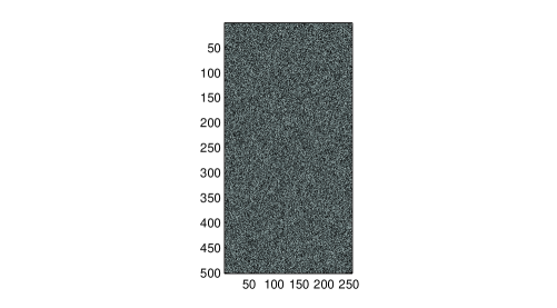
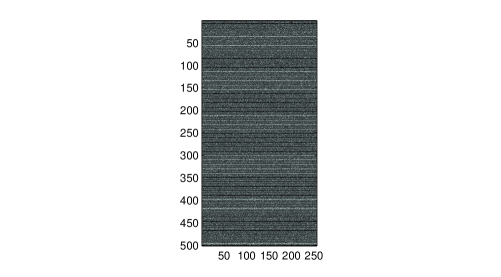
Figure 1: Business volume dynamics’ diagrams for the quantities sold, with $k=8$ business dimensions (i.e., $N=256$), with parameters: $b=2$, $\theta=14$, $\bar{Q}=30$, $\nu=30$, $\varepsilon_{2}=0.04$, $\delta=0.1$ and $\varepsilon_{1}=0.01$ (top diagram), $\varepsilon_{1}=0.3$ (bottom diagram). The grey scale is mapped automatically by the Software Fraclab from a Netlogo simulation, the darker regions corresponding to lower quantities sold, and lighter regions to higher quantities sold, transaction rounds are represented in the vertical while the spacial configuration of companies is represented horizontally. The 10,000 to 10,500 simulation steps are being shown.

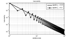
Figure 2: Lacunarity distributions for the previous figure diagrams.

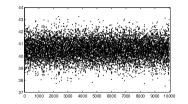
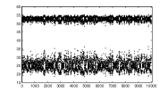
Figure 3: Time series diagrams for the quantum averages $\left\langle\hat{Q}_{h}\right\rangle_{\Psi_{t}}$, with $k=8$ business dimensions (i.e., $N=256$), with parameters: $b=2$, $\theta=14$, $\bar{Q}=30$, $\nu=30$, $\varepsilon_{2}=0.04$, $\delta=0.1$ and $\varepsilon_{1}=0.01$ (left diagram), $\varepsilon_{1}=0.3$ (right diagram). The 10,000 to 20,000 Netlogo simulation steps are being shown.

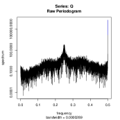
Figure 4: Raw (left) and smoothed (right) spectrograms for the previous figure data corresponding to the simulation with $\varepsilon_{1}=0.3$.

References

- [1] Baumol, W. and Benhabib, J., Chaos: Significance, Mechanism, and Economic Implications, Journal of Economic Perspectives, Vol. 3, No. 1, 1989, 77-105.
- [2] Berry, M.V., The Bakerian lecture, 1987: Quantum chaology, Proc. R. Soc. Lond. A vol.413, no.184, 1987, 183-198.
- [3] Copeland, T. E. and Weston, J.F., Financial Theory and Corporate Policy, Addison-Wesley Publishing Company, USA, 1983.
- [4] Chen, P., Empirical and theoretical evidence of economic chaos, System Dynamics Review, Vol. 4, No.1-2, 1988, 81-108.
- [5] Chen, P., Equilibrium Illusion, Economic Complexity and Evolutionary Foundation in Economic Analysis, Evol. Inst. Econ. Rev., 5(1), 2008, 81–127.
- [6] Day, R. H., Complex Economic Dynamics, Vol.1 - An Introduction to Dynamical Systems and Market Mechanisms, The MIT Press, USA, 1994.
- [7] Day, R. H., Complex Economic Dynamics, Vol.2 - An Introduction to Macroeconomic Dynamics, The MIT Press, USA, 2000.
- [8] Echelard, A., J. Levy-Véhel and I. Taralova, “Application of fractal tools for the classification of microscopical images of milk fat”, 2011, http://hal.inria.fr/inria-00559095/en/.
- [9] Gell-Mann, M. and Hartle, J.B., Decoherent Histories Quantum Mechanics with One ’Real’ Fine-Grained History, arXiv:1106.0767v3 [quant-ph], 2011.
- [10] Gardiner, C.W. and Zoller, P., Quantum Noise, A Handbook of Markovian and Non-Markovian Quantum Stochastic Methods with Applications to Quantum Optics, Springer, Germany, 2004.
- [11] Glauber, R.J., Coherent and incoherent states of the radiation field, Phys Rev., 131, 1963, 2766-2788.
- [12] Gonçalves, C.P., Quantum Financial Economics of Games of Strategy and Financial Decisions, arXiv:1202.2080v1 [q-fin.GN], 2012.
- [13] Hartle, J.B., Quantum Mechanics with Extended Probabilities, Phys. Rev. A, 78, 012108, 2008, [13 pages].
- [14] Joos, E., Zeh, H.D., Kiefer, C., Giulini, D., Kupsch, J. and Stamatescu, I.-O. (eds.), Decoherence and the Appearance of a Classical World in Quantum Theory, Springer, Germany, 2003.
- [15] Kaneko, K., Chaos as a Source of Compexity and Diversity in Evolution, Artificial Life I, 1994, 163-177
- [16] Kaneko, K. and I. Tsuda, Complex Systems: Chaos and Beyond, A Constructive Approach with Applications in Life Sciences, Springer, Germany, 2001.
- [17] Lambertini, L., Quantum Mechanics and Mathematical Economics are Isomorphic, wp 370, Dipartimento di Scienze Economiche, Università degli Studi di Bologna http://www2.dse.unibo.it/lamberti/johnvn.pdf, 2000.
- [18] Lorenz, H.-W., Nonlinear Dynamical Economics and Chaotic Motion, Springer, Germany, 1997.
- [19] Meyer, D.A., Quantum strategies, Phys. Rev. Lett. 82, 1999, 1052-1055.
- [20] Nash, J.F., Non-Cooperative Games, Annals of Mathematics, 54, 1951, 286-295.
- [21] Püu, T., 1997, Nonlinear Economic Dynamics, Springer, Germany, 1997.
- [22] Piotrowski, E.W. and Sladkowski, J., Quantum-like approach to financial risk: quantum anthropic principle, Acta Phys.Polon., B32, 2001, 3873.
- [23] Stöckmann, H.-J., Quantum Chaos, an introduction, Cambridge University Press, UK, 2000.
- [24] Sudarshan, E.C.G., Equivalence of Semiclassical and Quantum Mechanical Descriptions of Statistical Light Beams, Phys Rev. Lett. 10, 1963, 277-279.
- [25] Vicig, P., A Gambler’s Gain Prospects with Coherent Imprecise Previsions, Hüllermeier, E., Kruse, R. and Hoffmann, F. (Eds.), Information Processing and Management of Uncertainty in Knowledge-Based Systems, Theory and Methods, 13th International Conference, IPMU, Dortmund Germany, Proceedings Part I, Springer, Germany, 2010, 50-59.
- [26] Von Neumann, J. and Morgenstern, O., Theory of Games and Economic Behavior, Princeton University Press, USA, 1944.
- [27] Wolfram, S., A New Kind of Science, Wolfram Media, USA, 2002.