Large Scale Structure of the Universe

Abstract

Galaxies are not uniformly distributed in space. On large scales the Universe displays coherent structure, with galaxies residing in groups and clusters on scales of $\sim$1-3 $h^{-1}$ Mpc, which lie at the intersections of long filaments of galaxies that are $>$10 $h^{-1}$ Mpc in length. Vast regions of relatively empty space, known as voids, contain very few galaxies and span the volume in between these structures. This observed large scale structure depends both on cosmological parameters and on the formation and evolution of galaxies. Using the two-point correlation function, one can trace the dependence of large scale structure on galaxy properties such as luminosity, color, stellar mass, and track its evolution with redshift. Comparison of the observed galaxy clustering signatures with dark matter simulations allows one to model and understand the clustering of galaxies and their formation and evolution within their parent dark matter halos. Clustering measurements can determine the parent dark matter halo mass of a given galaxy population, connect observed galaxy populations at different epochs, and constrain cosmological parameters and galaxy evolution models. This chapter describes the methods used to measure the two-point correlation function in both redshift and real space, presents the current results of how the clustering amplitude depends on various galaxy properties, and discusses quantitative measurements of the structures of voids and filaments. The interpretation of these results with current theoretical models is also presented.

1 Historical Background

Large scale structure is defined as the structure or inhomogeneity of the Universe on scales larger than that of a galaxy. The idea of whether galaxies are distributed uniformly in space can be traced to Edwin Hubble, who used his catalog of 400 “extragalactic nebulae” to test the homogeneity of the Universe (Hubble, 1926), finding it to be generally uniform on large scales. In 1932, the larger Shapley-Ames catalog of bright galaxies was published (Shapley & Ames, 1932), in which the authors note “the general unevenness in distribution” of the galaxies projected onto the plane of the sky and the roughly factor of two difference in the numbers of galaxies in the northern and southern galactic hemispheres. Using this larger statistical sample, Hubble (1934) noted that on angular scales less than $\sim$10^∘ there is an excess in the number counts of galaxies above what would be expected for a random Poisson distribution, though the sample follows a Gaussian distribution on larger scales. Hence, while the Universe appears to be homogeneous on the largest scales, on smaller scales it is clearly clumpy.

Measurements of large scale structure took a major leap forward with the Lick galaxy catalog produced by Shane & Wirtanen (1967), which contained information on roughly a million galaxies obtained using photographic plates at the 0.5m refractor at Lick Observatory. Seldner et al. (1977) published maps of the counts of galaxies in angular cells across the sky (see Fig. 1), which showed in much greater detail that the projected distribution of galaxies on the plane of the sky is not uniform. The maps display a rich structure with a foam-like pattern, containing possible walls or filaments with long strands of galaxies, clusters, and large empty regions. The statistical spatial distribution of galaxies from this catalog and that of Zwicky et al. (1968) was analyzed by Jim Peebles and collaborators in a series of papers (e.g., Peebles, 1975) that showed that the angular two-point correlation function (defined below) roughly follows a power law distribution over angular scales of $\sim$0.1^∘– 5^∘. In these papers it was discovered that the clustering amplitude is lower for fainter galaxy populations, which likely arises from larger projection effects along the line of sight. As faint galaxies typically lie at larger distances, the projected clustering integrates over a wider volume of space and therefore dilutes the effect.

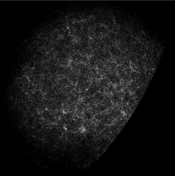
Figure 1: Angular distribution of counts of galaxies brighter than $B\sim 19$ on the plane of the sky, reconstructed from the Lick galaxy catalog (from Seldner et al. 1997). This image shows the number of galaxies observed in 10^′ $\times$ 10^′ cells across the northern galactic hemisphere, where brighter cells contain more galaxies. The northern galactic pole is at the center, with the galactic equator at the edge. The distribution of galaxies is clearly not uniform; clumps of galaxies are seen in white, with very few galaxies observed in the dark regions between.

These results in part spurred the first large scale redshift surveys, which obtained optical spectra of individual galaxies in order to measure the redshifts and spatial distributions of large galaxy samples. Pioneering work by Gregory & Thompson (1978) mapped the three-dimensional spatial distribution of 238 galaxies around and towards the Coma/Abell 1367 supercluster. In addition to surveying the galaxies in the supercluster, they found that in the foreground at lower redshift there were large regions ($>20$ $h^{-1}$ Mpc, shown well in their Figure 2a) with no galaxies, which they termed ’voids’. Joeveer et al. (1978) used redshift information from Sandage & Tammann (1975) to map the three-dimensional distribution of galaxies on large scales in the southern galactic hemisphere. They mapped four separate volumes that included clusters as well as field galaxies and showed that across large volumes, galaxies are clearly clustered in three dimensions and often form ’chains’ of clusters (now recognized as filaments).

Two additional redshifts surveys were the KOS survey (Kirshner, Oemler, Schechter; Kirshner et al., 1978) and the original CfA survey (Center for Astrophysics; Davis et al., 1982). The KOS survey measured redshifts for 164 galaxies brighter than magnitude 15 in eight separate fields on the sky, covering a total of 15 deg². Part of the motivation for the survey was to study the three dimensional spatial distribution of galaxies, about which the authors note that “although not entirely unexpected, it is striking how strongly clustered our galaxies are in velocity space,” as seen in strongly peaked one dimensional redshift histograms in each field.

The original CfA survey, completed in 1982, contained redshifts for 2,400 galaxies brighter than magnitude 14.5 across the north and south galactic poles, covering a total of 2.7 steradians. The major aims of the survey were cosmological and included quantifying the clustering of galaxies in three dimensions. This survey produced large area, moderately deep three dimensional maps of large scale structure (see Fig. 2), in which one could identify galaxy clusters, voids, and an apparent “filamentary connected structure” between groups of galaxies, which the authors caution could be random projections of distinct structures (Davis et al., 1982). This paper also performed a comparison of the so-called “complex topology” of the large scale structure seen in the galaxy distribution with that seen in N-body dark matter simulations, paving the way for future studies of theoretical models of structure formation.

The second CfA redshift survey, which ran from 1985 to 1995, contained spectra for $\sim$5,800 galaxies and revealed the existence of the so-called “Great Wall”, a supercluster of galaxies that extends over 170 $h^{-1}$ Mpc, the width of the survey (Geller & Huchra, 1989). Large underdense voids were also commonly found, with a density 20% of the mean density.

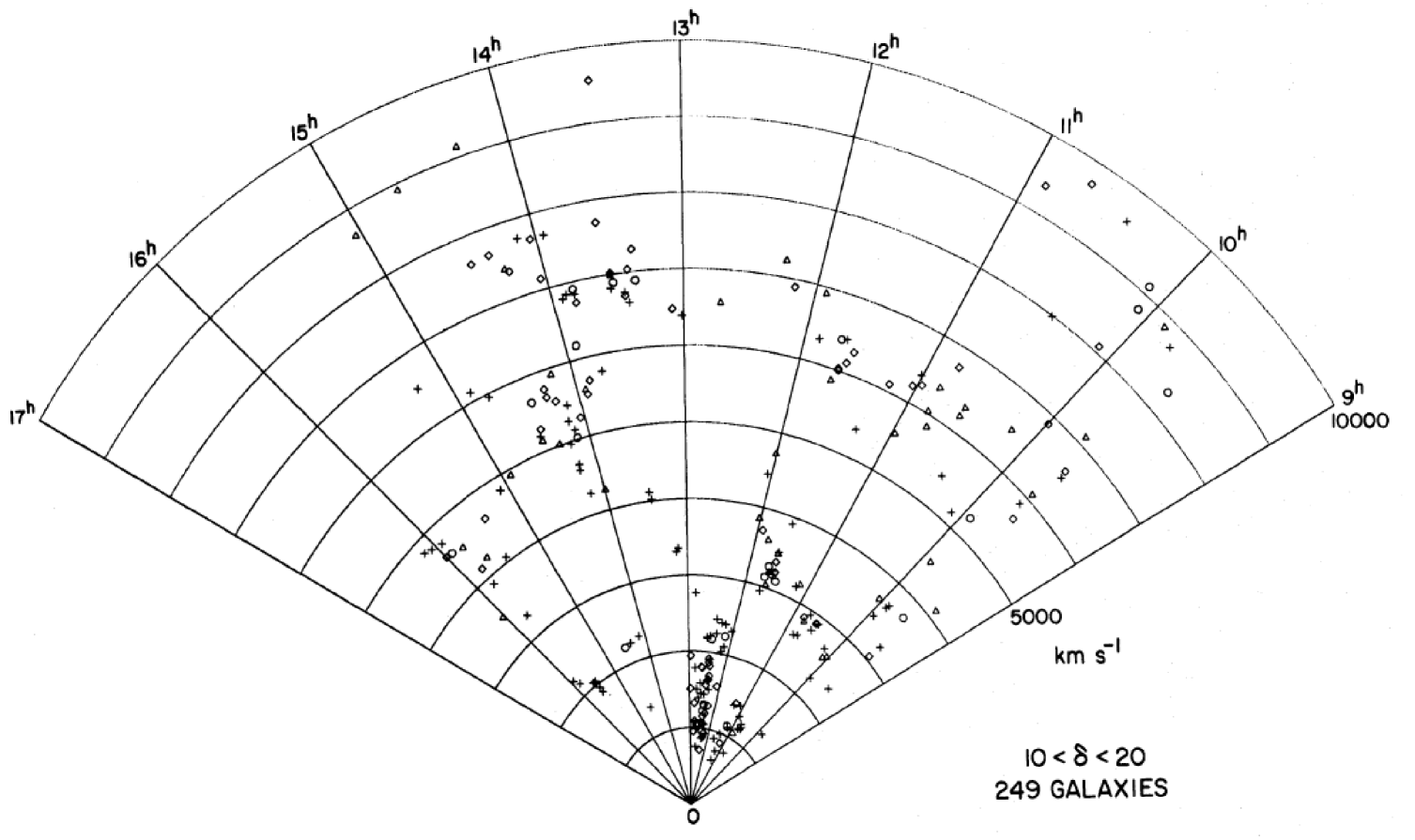
Figure 2: Distribution of galaxies in redshift space from the original CfA galaxy redshift survey (from Davis et al. 1982). Plotted are 249 galaxies as a function of observed velocity (corresponding to a given redshift) versus right ascension for a wedge in declination of 10^∘$<\delta<$ 20^∘.

Redshift surveys have rapidly progressed with the development of multi-object spectrographs, which allow simultaneous observations of hundreds of galaxies, and larger telescopes, which allow deeper surveys of both lower luminosity nearby galaxies and more distant, luminous galaxies. At present the largest redshift surveys of galaxies at low redshift are the Two Degree Field Galaxy Redshift Survey (2dFGRS, Colless et al., 2001) and the Sloan Digital Sky Survey (SDSS, York et al., 2000), which cover volumes of $\sim 4\times 10^{7}\ h^{3}$ Mpc^-3 and $\sim 2\times 10^{8}\ h^{3}$ Mpc^-3 with spectroscopic redshifts for $\sim$220,000 and a million galaxies, respectively. These surveys provide the best current maps of large scale structure in the Universe today (see Fig. 3), revealing a sponge-like pattern to the distribution of galaxies (Gott et al., 1986). Voids of $\sim$10 $h^{-1}$ Mpc are clearly seen, containing very few galaxies. Filaments stretching greater than 10 $h^{-1}$ Mpc surround the voids and intersect at the locations of galaxy groups and clusters.

The prevailing theoretical paradigm regarding the existence of large scale structure is that the initial fluctuations in the energy density of the early Universe, seen as temperature deviations in the cosmic microwave background, grow through gravitational instability into the structure seen today in the galaxy density field. The details of large scale structure – the sizes, densities, and distribution of the observed structure – depend both on cosmological parameters such as the matter density and dark energy as well as on the physics of galaxy formation and evolution. Measurements of large scale structure can therefore constrain both cosmology and galaxy evolution physics.

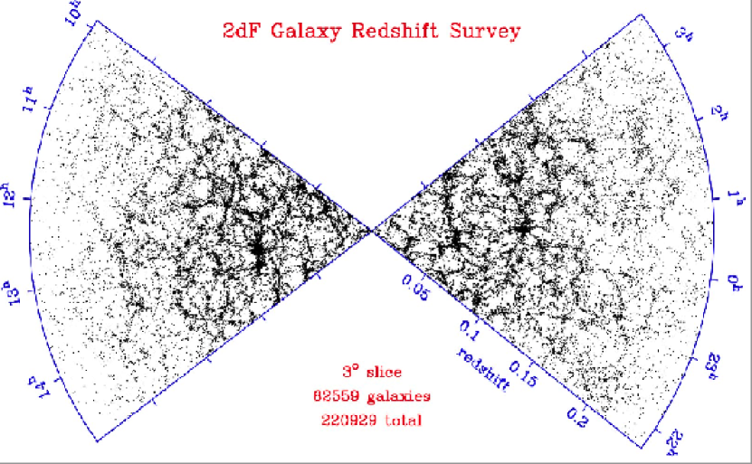
Figure 3: The spatial distribution of galaxies as a function of redshift and right ascension (projected through 3^∘ in declination) from the 2dF Galaxy Redshift Survey (from Colless et al. 2004).

2 The Two-Point Correlation Function

In order to quantify the clustering of galaxies, one must survey not only galaxies in clusters but rather the entire galaxy density distribution, from voids to superclusters. The most commonly used quantitative measure of large scale structure is the galaxy two-point correlation function, $\xi(r)$, which traces the amplitude of galaxy clustering as a function of scale. $\xi(r)$ is defined as a measure of the excess probability $dP$, above what is expected for an unclustered random Poisson distribution, of finding a galaxy in a volume element $dV$ at a separation $r$ from another galaxy,

$$dP=n[1+\xi(r)]dV,$$ (1)

where $n$ is the mean number density of the galaxy sample in question (Peebles, 1980). Measurements of $\xi(r)$ are generally performed in comoving space, with $r$ having units of $h^{-1}$ Mpc. The Fourier transform of the two-point correlation function is the power spectrum, which is often used to describe density fluctuations observed in the cosmic microwave background.

To measure $\xi(r)$, one counts pairs of galaxies as a function of separation and divides by what is expected for an unclustered distribution. To do this one must construct a “random catalog” that has the identical three dimensional coverage as the data – including the same sky coverage and smoothed redshift distribution – but is populated with randomly-distribution points. The ratio of pairs of galaxies observed in the data relative to pairs of points in the random catalog is then used to estimate $\xi(r)$. Several different estimators for $\xi(r)$ have been proposed and tested. An early estimator that was widely used is from Davis & Peebles (1983):

$$\xi=\frac{n_{R}}{n_{D}}\frac{DD}{DR}-1,$$ (2)

where $DD$ and $DR$ are counts of pairs of galaxies (in bins of separation) in the data catalog and between the data and random catalogs, and $n_{D}$ and $n_{R}$ are the mean number densities of galaxies in the data and random catalogs. Hamilton (1993) later introduced an estimator with smaller statistical errors,

$$\xi=\frac{DD\ RR}{(DR)^{2}}-1,$$ (3)

where $RR$ is the count of pairs of galaxies as a function of separation in the random catalog. The most commonly-used estimator is from Landy & Szalay (1993),

$$\xi=\frac{1}{RR}\left[DD\left(\frac{n_{R}}{n_{D}}\right)^{2}-2DR\left(\frac{n_{R}}{n_{D}}\right)+RR\right].$$ (4)

This estimator has been shown to perform as well as the Hamilton estimator (Eqn. 3), and while it requires more computational time it is less sensitive to the size of the random catalog and handles edge corrections well, which can affect clustering measurements on large scales (Kerscher et al., 2000).

As can be seen from the form of the estimators given above, measuring $\xi(r)$ depends sensitively on having a random catalog which accurately reflects the various spatial and redshift selection affects in the data. These can include effects such as edges of slitmasks or fiber plates, overlapping slitmasks or plates, gaps between chips on the CCD, and changes in spatial sensitivity within the detector (i.e., the effective radial dependence within X-ray detectors). If one is measuring a full three-dimensional correlation function (discussed below) then the random catalog must also accurately include the redshift selection of the data. The random catalog should also be large enough to not introduce Poisson error in the estimator. This can be checked by ensuring that the RR pair counts in the smallest bin are high enough such that Poisson errors are subdominant.

3 Angular Clustering

The spatial distribution of galaxies can be measured either in two dimensions as projected onto the plane of the sky or in three dimensions using the redshift of each galaxy. As it can be observationally expensive to obtain spectra for large samples of (particularly faint) galaxies, redshift information is not always available for a given sample. One can then measure the two-dimensional projected angular correlation function $\omega(\theta)$, defined as the probability above Poisson of finding two galaxies with an angular separation $\theta$:

$$dP=N[1+\omega(\theta)]d\Omega$$ (5)

where $N$ is the mean number of galaxies per steradian and d$\Omega$ is the solid angle of a second galaxy at a separation $\theta$ from a randomly chosen galaxy.

Measurements of $\omega(\theta)$ are known to be low by an additive factor known as the “integral constraint”, which results from using the data sample itself (which often does not cover large areas of the sky) to estimate the mean galaxy density. This correction becomes important on angular scales comparable to the survey size; on much smaller scales it is negligible. One can either restrict measurements of the angular clustering to scales where the integral constraint is not important or estimate the amplitude of the integral constraint correction by doubly integrating an assumed power law form of $\omega(\theta)$ over the survey area, $\Omega$, using

$$AC=\frac{1}{\Omega}\int\int\omega(\theta)d\Omega_{1}d\Omega_{2},$$ (6)

where $\Omega$ is the area subtended by the survey. In practice, this can be numerically estimated over the survey geometry using the random catalog itself (see Roche & Eales 1999 for details).

The projected angular two-point correlation function, $\omega(\theta)$, can generally be fit with a power law,

$$\omega(\theta)=A_{\omega}\theta^{\delta}$$ (7)

where A is the clustering amplitude at a given scale (often 1^′) and $\delta$ is the slope of the correlation function.

From measurements of $\omega(\theta)$ one can infer the three-dimensional spatial two-point correlation function, $\xi(r)$, if the redshift distribution of the sources is well known. The two-point correlation function, $\xi(r)$, is usually fit as a power law, $\xi(r)=(r/r_{0})^{-\gamma}$, where $r_{0}$ is the characteristic scale-length of the galaxy clustering, defined as the scale at which $\xi=1$. As the two-dimensional galaxy clustering seen in the plane of the sky is a projection of the three-dimensional clustering, $\omega(\theta)$ is directly related to its three-dimensional analog $\xi(r)$. For a given $\xi(r)$, one can predict the amplitude and slope of $\omega(\theta)$ using Limber’s equation, effectively integrating $\xi(r)$ along the redshift direction (e.g. Peebles 1980). If one assumes $\xi(r)$ (and thus $\omega(\theta)$) to be a power law over the redshift range of interest, such that

$$\xi(r,z)=\left[\frac{r_{0}(z)}{r}\right]^{\gamma},$$ (8)

then

$$w(\theta)=\sqrt{\pi}\frac{\Gamma[(\gamma-1)/2]}{\Gamma(\gamma/2)}\frac{A}{\theta^{\gamma-1}},$$ (9)

where $\Gamma$ is the usual gamma function. The amplitude factor, $A$, is given by

$$A=\frac{\int_{0}^{\infty}r_{0}^{\gamma}(z)g(z)\left(\frac{dN}{dz}\right)^{2}dz}{\left[\int_{0}^{\infty}\left(\frac{dN}{dz}\right)dz\right]^{2}}$$ (10)

where $dN/dz$ is the number of galaxies per unit redshift interval and $g(z)$ depends on $\gamma$ and the cosmological model:

$$g(z)=\left(\frac{dz}{dr}\right)r^{(1-\gamma)}F(r).$$ (11)

Here $F(r)$ is the curvature factor in the Robertson-Walker metric,

$$ds^{2}=c^{2}dt^{2}-a^{2}[dr^{2}/F(r)^{2}+r^{2}d\theta^{2}+r^{2}sin^{2}\theta d\phi^{2}].$$ (12)

If the redshift distribution of sources, $dN/dz$, is well known, then the amplitude of $\omega(\theta)$ can be predicted for a given power law model of $\xi(r)$, such that measurements of $\omega(\theta)$ can be used to place constraints on the evolution of $\xi(r)$.

Interpreting angular clustering results can be difficult, however, as there is a degeneracy between the inherent clustering amplitude and the redshift distribution of the sources in the sample. For example, an observed weakly clustered signal projected on the plane of the sky could be due either to the galaxy population being intrinsically weakly clustered and projected over a relatively short distance along the line of sight, or it could result from an inherently strongly clustered distribution integrated over a long distance, which would wash out the signal. The uncertainty on the redshift distribution is therefore often the dominant error in analyses using angular clustering measurements. The assumed galaxy redshift distribution ($dN/dz$) has varied widely in different studies, such that similar observed angular clustering results have led to widely different conclusions. A further complication is that each sample usually spans a large range of redshifts and is magnitude-limited, such that the mean intrinsic luminosity of the galaxies is changing with redshift within a sample, which can hinder interpretation of the evolution of clustering measured in $\omega(\theta)$ studies.

Many of the first measurements of large scale structure were studies of angular clustering. One of the earliest determinations was the pioneering work of Peebles (1975) using photographic plates from the Lick survey (Fig. 1). They found $\omega(\theta)$ to be well fit by a power law with a slope of $\delta=-0.8$. Later studies using CCDs were able to reach deeper magnitude limits and found that fainter galaxies had a lower clustering amplitude. One such study was conducted by Postman et al. (1998), who surveyed a contiguous 4^∘ by 4^∘ field to a depth of $I_{\rm AB}=24$ mag, reaching to $z\sim 1$. Later surveys that covered multiple fields on the sky found similar results. The lower clustering amplitude observed for galaxies with fainter apparent magnitudes can in principle be due either to clustering being a function of luminosity and/or a function of redshift. To disentangle this dependence, each author assumes a $dN/dz$ distribution for galaxies as a function of apparent magnitude and then fits the observed $\omega(\theta)$ with different models of the redshift dependence of clustering. While many authors measure similar values of the dependence of $\omega(\theta)$ on apparent magnitude, due to differences in the assumed $dN/dz$ distributions different conclusions are reached regarding the amount of luminosity and redshift dependence to galaxy clustering. Additionally, quoted error bars on the inferred values of $r_{0}$ generally include only Poisson and/or cosmic variance error estimates, while the dominant error is often the lack of knowledge of $dN/dz$ for the particular sample in question.

Because of the sensitivity of the inferred value of $r_{0}$ on the redshift distribution of sources, it is preferable to measure the three dimensional correlation function. While it is much easier to interpret three dimensional clustering measurements, in cases where it is still not feasible to obtain redshifts for a large fraction of galaxies in the sample, angular clustering measurements are still employed. This is currently the case in particular with high redshift and/or very dusty, optically-obscured galaxy samples, such as sub-millimeter galaxies (e.g., Brodwin et al., 2008; Maddox et al., 2010). However, without knowledge of the redshift distribution of the sources, these measurements are hard to interpret.

4 Real and Redshift Space Clustering

Measurements of the two-point correlation function use the redshift of a galaxy, not its distance, to infer its location along the line of sight. This introduces two complications: one is that a cosmological model has to be assumed to convert measured redshifts to inferred distances, and the other is that peculiar velocities introduce redshift space distortions in $\xi$ parallel to the line of sight Sargent & Turner (1977). On the first point, errors on the assumed cosmology are generally subdominant, so that while in theory one could assume different cosmological parameters and check which results are consistent with the assumed values, that is generally not necessary. On the second point, redshift space distortions can be measured to constrain cosmological parameters, and they can also be integrated over to recover the underlying real space correlation function.

On small spatial scales ($\lesssim 1$ $h^{-1}$ Mpc), within collapsed virialized overdensities such as groups and clusters, galaxies have large random motions relative to each other. Therefore while all of the galaxies in the group or cluster have a similar physical distance from the observer, they have somewhat different redshifts. This causes an elongation in redshift space maps along the line of sight within overdense regions, which is referred to as “Fingers of God”. The result is that groups and clusters appear to be radially extended along the line of sight towards the observer. This effect can be seen clearly in Fig. 4, where the lower left panel shows galaxies in redshift space with large “Fingers of God” pointing back to the observer, while in the lower right panel the “Fingers of God” have been modeled and removed. Redshift space distortions are also seen on larger scales ($\gtrsim 1$ $h^{-1}$ Mpc) due to streaming motions of galaxies that are infalling onto structures that are still collapsing. Adjacent galaxies will all be moving in the same direction, which leads to coherent motion and causes an apparent contraction of structure along the line of sight in redshift space (Kaiser, 1987), in the opposite sense as the “Fingers of God”.

Figure 4: An illustration of the “Fingers of God” (FoG), or elongation of virialized structures along the line of sight, from Tegmark et al. (2004). Shown are galaxies from a slice of the SDSS sample (projected here through the declination direction) in two dimensional comoving space. The top row shows all galaxies in this slice (67,626 galaxies in total), while the bottom row shows galaxies that have been identified as having “Fingers of God”. The right column shows the position of these galaxies in this space after modeling and removing the effects of the “Fingers of God”. The observer is located at (x,y=0,0), and the “Fingers of God” effect can be seen in the lower left panel as the positions of galaxies being radially smeared along the line of sight toward the observer.

Redshift space distortions can be clearly seen in measurements of galaxy clustering. While redshift space distortions can be used to uncover information about the underlying matter density and thermal motions of the galaxies (discussed below), they complicate a measurement of the two-point correlation function in real space. Instead of $\xi(r)$, what is measured is $\xi(s)$, where $s$ is the redshift space separation between a pair of galaxies. While some results in the literature present measurements of $\xi(s)$ for various galaxy populations, it is not straightforward to compare results for different galaxy samples and different redshifts, as the amplitude of redshift space distortions differs depending on the galaxy type and redshift. Additionally, $\xi(s)$ does not follow a power law over the same scales as $\xi(r)$, as redshift space distortions on both small and large scales decrease the amplitude of clustering relative to intermediate scales.

The real-space correlation function, $\xi(r)$, measures the underlying physical clustering of galaxies, independent of any peculiar velocities. Therefore, in order to recover the real-space correlation function, one can measure $\xi$ in two dimensions, both perpendicular to and along the line of sight. Following Fisher et al. (1994), ${\bf v_{1}}$ and ${\bf v_{2}}$ are defined to be the redshift positions of a pair of galaxies, ${\bf s}$ to be the redshift space separation (${\bf v_{1}}-{\bf v_{2}}$), and ${\bf l}=\frac{1}{2}$(${\bf v_{1}}+{\bf v_{2}})$ to be the mean distance to the pair. The separation between the two galaxies across ($r_{p}$) and along ($\pi$) the line of sight are defined as

$$\pi=\frac{{\bf s}\cdot{\bf l}}{{\bf|l|}},$$ (13)

$$r_{p}=\sqrt{{\bf s}\cdot{\bf s}-\pi^{2}}.$$ (14)

One can then compute pair counts over a two-dimensional grid of separations to estimate $\xi(r_{p},\pi)$. $\xi(s)$, the one-dimensional redshift space correlation function, is then equivalent to the azimuthal average of $\xi(r_{p},\pi)$.

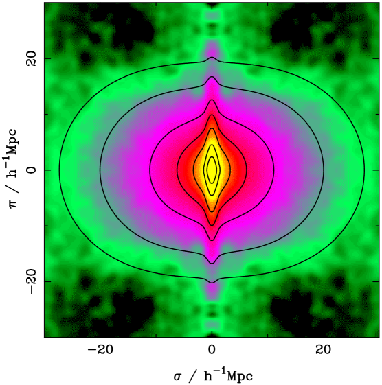
Figure 5: The two-dimensional redshift space correlation function from 2dFGRS (Peacock et al., 2001). Shown is $\xi(r_{p},\pi)$ (in the figure $\sigma$ is used instead of $r_{p}$), the correlation function as a function of separation across ($\sigma$ or $r_{p}$) and along ($\pi$) the line of sight. Contours show lines of constant $\xi$ at $\xi=$10, 5, 2, 1, 0.5, 0.2, 0.1. Data from the first quadrant (upper right) are reflected about both the $\sigma$ and $\pi$ axes, to emphasize deviations from circular symmetry due to redshift space distortions.

An example of a measurement of $\xi(r_{p},\pi)$ is shown in Fig. 5. Plotted is $\xi$ as a function of separation $r_{p}$ (defined in this figure to be $\sigma$) across and $\pi$ along the line of sight. What is usually shown is the upper right quadrant of this figure, which here has been reflected about both axes to emphasize the distortions. Contours of constant $\xi$ follow the color-coding, where yellow corresponds to large $\xi$ values and green to low values. On small scales across the line of sight ($r_{p}$ or $\sigma<\sim 2$ $h^{-1}$ Mpc) the contours are clearly elongated in the $\pi$ direction; this reflects the “Fingers of God” from galaxies in virialized overdensities. On large scales across the line of sight ($r_{P}$ or $\sigma>\sim 10$ $h^{-1}$ Mpc) the contours are flattened along the line of sight, due to “the Kaiser effect”. This indicates that galaxies on these linear scales are coherently streaming onto structures that are still collapsing.

As this effect is due to the gravitational infall of galaxies onto massive forming structures, the strength of the signature depends on $\Omega_{\rm matter}$. Kaiser (1987) derived that the large-scale anisotropy in the $\xi(r_{p},\pi)$ plane depends on $\beta\equiv\Omega_{\rm matter}/b$ on linear scales, where $b$ is the bias or the ratio of density fluctuations in the galaxy population relative to that of dark matter (discussed further in the next section below). Anisotropies are quantified using the multipole moments of $\xi(r_{p},\pi)$, defined as

$$\xi_{l}(s)=(2l+1)/2\int{\xi(r_{p},\pi)\ P_{l}(\cos\theta)\ d\cos\theta},$$ (15)

where $s$ is the distance as measured in redshift space, $P_{l}$ are Legendre polynomials, and $\theta$ is the angle between $s$ and the line of sight. The ratio $\xi_{2}$/$\xi_{0}$, the quadrupole to monopole moments of the two-point correlation function, is related to $\beta$ in a simple manner using linear theory (Hamilton, 1998):

$$\xi_{2}/\xi_{0}=f(n)\frac{\frac{4}{3}\beta+\frac{4}{7}\beta^{2}}{1+\frac{2}{3}\beta+\frac{1}{5}\beta^{2}}$$ (16)

where $f(n)$ =(3+$n)/n$ and $n$ is the index of the two-point correlation function in a power-law form: $\xi\propto r^{-(3+n)}$ (Hamilton, 1992).

Peacock et al. (2001) find using measurements of the quadrupole-to-monopole ratio in the 2dFGRS data (see Fig. 5) that $\beta=0.43\pm 0.07$. For a bias value of around unity (see Section 5 below), this implies a low value of $\Omega_{\rm matter}\sim 0.3$. Similar measurements have been made with clustering measurements using data from the SDSS. Very large galaxy samples are needed to detect this coherent infall and obtain robust estimates of $\beta$. At higher redshift, Guzzo et al. (2008) find $\beta=0.70\pm 0.26$ at $z=0.77$ using data from the VVDS and argue that measurements of $\beta$ as a function of redshift can be used to trace the expansion history of the Universe. We return to the discussion of redshift space distortions on small scales below in Section 6.3.

What is often desired, however, is a measurement of the real space clustering of galaxies. To recover $\xi(r)$ one can then project $\xi(r_{p},\pi)$ along the $r_{p}$ axis. As redshift space distortions affect only the line-of-sight component of $\xi(r_{p},\pi)$, integrating over the $\pi$ direction leads to a statistic $w_{p}(r_{p})$, which is independent of redshift space distortions. Following Davis & Peebles (1983),

$$w_{p}(r_{p})=2\int_{0}^{\infty}d\pi\ \xi(r_{p},\pi)=2\int_{0}^{\infty}dy\ \xi(r_{p}^{2}+y^{2})^{1/2},$$ (17)

where $y$ is the real-space separation along the line of sight. If $\xi(r)$ is modeled as a power-law, $\xi(r)=(r/r_{0})^{-\gamma}$, then $r_{0}$ and $\gamma$ can be readily extracted from the projected correlation function, $w_{p}(r_{p})$, using an analytic solution to Equation 17:

$$w_{p}(r_{p})=r_{p}\left(\frac{r_{0}}{r_{p}}\right)^{\gamma}\frac{\Gamma(\frac{1}{2})\Gamma(\frac{\gamma-1}{2})}{\Gamma(\frac{\gamma}{2})},$$ (18)

where $\Gamma$ is the usual gamma function. A power-law fit to $w_{p}(r_{p})$ will then recover $r_{0}$ and $\gamma$ for the real-space correlation function, $\xi(r)$. In practice, Equation 17 is not integrated to infinite separations. Often values of $\pi_{\rm max}$ are $\sim$40-80 $h^{-1}$ Mpc, which includes most correlated pairs. It is worth noting that the values of $r_{0}$ and $\gamma$ inferred are covariant. One must therefore be careful when comparing clustering amplitudes of different galaxy populations; simply comparing the $r_{0}$ values may be misleading if the correlation function slopes are different. It is often preferred to compare the galaxy bias instead (see next section).

As a final note on measuring the two-point correlation function, as can be seen from Fig. 3, flux-limited galaxy samples contain a higher density of galaxies at lower redshift. This is purely an observational artifact, due to the apparent magnitude limit including intrinsically lower luminosity galaxies nearby, while only tracing the higher luminosity galaxies further away. As discussed below in Section 6, because the clustering amplitude of galaxies depends on their properties, including luminosity, one would ideally only measure $\xi(r)$ in volume-limited samples, where galaxies of the same absolute magnitude are observed throughout the entire volume of the sample, including at the highest redshifts. Therefore often the full observed galaxy population is not used in measurements of $\xi(r)$, rather volume-limited sub-samples are created where all galaxies are brighter than a given absolute magnitude limit. This greatly facilitates the theoretical interpretation of clustering measurements (see Section 8) and the comparison of results from different surveys.

5 Galaxy Bias

It was realized decades ago that the spatial clustering of observable galaxies need not precisely mirror the clustering of the bulk of the matter in the Universe. In its most general form, the galaxy density can be a non-local and stochastic function of the underlying dark matter density. This galaxy “bias” – the relationship between the spatial distribution of galaxies and the underlying dark matter density field – is a result of the varied physics of galaxy formation which can cause the spatial distribution of baryons to differ from that of dark matter. Stochasticity appears to have little effect on bias except for adding extra variance (e.g., Scoccimarro, 2000), and non-locality can be taken into account to first order by using smoothed densities over larger scales. In this approximation, the smoothed galaxy density contrast is a general function of the underlying dark matter density contrast on some scale:

$$\delta_{g}=f(\delta),$$ (19)

where $\delta\equiv(\rho/\bar{\rho})-1$ and $\bar{\rho}$ is the mean mass density on that scale. If we assume $f(\delta)$ is a linear function of $\delta$, then we can define the linear galaxies bias $b$ as the ratio of the mean overdensity of galaxies to the mean overdensity of mass,

$$b=\delta_{g}/\delta,$$ (20)

and can in theory depend on scale and galaxy properties such as luminosity, morphology, color and redshift. In terms of the correlation function, the linear bias is defined as the square root of the ratio of the two-point correlation function of the galaxies relative to the dark matter:

$$b=(\xi_{\rm gal}/\xi_{\rm dark\ matter})^{1/2}$$ (21)

and is a function of scale. Note that $\xi_{\rm dark\ matter}$ is the Fourier transform of the dark matter power spectrum. The bias of galaxies relative to dark matter is often referred to as the absolute bias, as opposed to the relative bias between galaxy populations (discussed below).

The concept of galaxies being a biased tracer of the underlying total mass field (which is dominated by dark matter) was introduced by Kaiser (1984) in an attempt to reconcile the different clustering scale lengths of galaxies and rich clusters, which could not both be unbiased tracers of mass. Kaiser (1984) show that clusters of galaxies would naturally have a large bias as a result of being rare objects which formed at the highest density peaks of the mass distribution, above some critical threshold. This idea is further developed analytically by Bardeen et al. (1986) for galaxies, who show that for a Gaussian distribution of initial mass density fluctuations, the peaks which first collapse to form galaxies will be more clustered than the underlying mass distribution. Mo & White (1996) use extended Press-Schechter theory to determine that the bias depends on the mass of the dark matter halo as well as the epoch of galaxy formation and that a linear bias is a decent approximation well into the non-linear regime where $\delta>$1. The evolution of bias with redshift is developed in theoretical work by Fry (1996) and Tegmark & Peebles (1998), who find that the bias is naturally larger at earlier epochs of galaxy formation, as the first galaxies to form will collapse in the most overdense regions of space, which are biased (akin to mountain peaks being clustered). They further show that regardless of the initial amplitude of the bias factor, with time galaxies will become unbiased tracers of the mass distribution ($b\rightarrow$1 as $t\rightarrow\infty$). Additionally, Mann et al. (1998) find that while bias is generally scale-dependent, the dependence is weak and on large scales the bias tends towards a constant value.

A galaxy population can be “anti-biased” if $b<1$, indicating that galaxies are less clustered than the dark matter distribution. As discussed below, this appears to be the case for some galaxy samples at low redshift. The galaxy bias of a given observational sample is often inferred by comparing the observed clustering of galaxies with the clustering of dark matter measured in a cosmological simulation. Therefore the bias depends on the cosmological model used in the simulation. The dominant relevant cosmological parameter is $\sigma_{8}$, defined as the standard deviation of galaxy count fluctuations in a sphere of radius 8 $h^{-1}$ Mpc, and the absolute bias value inferred can be simply scaled with the assumed value of $\sigma_{8}$. As discussed in section 9.1 below, the absolute galaxy bias can also be estimated from the data directly, without having to resort to comparisons with cosmological simulations, by using the ratio of the two-point and three-point correlation functions, which have different dependencies on the bias. While this measurement can be somewhat noisy, it has the advantage of not assuming a cosmological model from which to derive the dark matter clustering. This measurement is performed by Verde et al. (2002) and Gaztañaga et al. (2005), who find that galaxies in 2dFGRS have a linear bias value very close to unity on large scales.

The relative bias between different galaxy populations can also be measured and is defined as the ratio of the clustering of one population relative to another. This is often measured using the ratio of the projected correlation functions of each population:

$$b_{\rm gal1/gal2}=(w_{p,\rm gal1}/w_{p,\rm gal2})^{1/2},$$ (22)

where both measurements of $w_{p}(r_{p})$ have been integrated to the same value of $\pi_{max}$. The relative bias is used to compare the clustering of galaxies as a function of observed parameters and does not refer to the clustering of dark matter. It is a useful way to compare the observed clustering for different galaxy populations without having to rely on an assumed value of $\sigma_{8}$ for the dark matter.

6 The Dependence of Clustering on Galaxy Properties

The two-point correlation function has long been known to depend on galaxy properties and can vary as a function of galaxy luminosity, morphological or spectral type, color, stellar mass, and redshift. The general trend is that galaxies that are more luminous, early-type, bulge-dominated, optically red, and/or higher stellar mass are more clustered than galaxies that are less luminous, late-type, disk-dominated, optically blue, and/or lower stellar mass. Presented below are relatively recent results indicating how clustering properties depend on galaxy properties from the largest redshifts surveys currently available. The physical interpretation behind these trends is presented in Section 8 below.

6.1 Luminosity Dependence

Fig. 3 shows the large scale structure reflected in the galaxy distribution at low redshift. What is plotted is the spatial distribution of galaxies in a flux-limited sample, meaning that all galaxies down to a given apparent magnitude limit are included. This results in the apparent lack of galaxies or structure at higher redshift in the figure, as at large distances only the most luminous galaxies will be included in a flux-limited sample. In order to robustly determine the underlying clustering, one should, if possible, create volume-limited subsamples in which galaxies of the same luminosity can be detected at all redshifts. In this way the mean luminosity of the sample does not change with redshift and galaxies at all redshifts are weighted equally.

The left panel of Fig. 6 shows the projected correlation function, $w_{p}(r_{p})$, for galaxies in SDSS in volume-limited subsamples corresponding to different absolute magnitude ranges. The more luminous galaxies are more strongly clustered across a wide range in absolute optical magnitude, from $-17<M_{r}<-23$. Power law fits on scales from $\sim$0.1 $h^{-1}$ Mpc to $\sim$10 $h^{-1}$ Mpc show that while the clustering amplitude depends sensitively on luminosity, the slope does not. Only in the brightest and faintest magnitude bins does the slope deviate from $\gamma\sim 1.8$ and have a steeper value of $\gamma\sim 2.0$. Across this magnitude range $r_{0}$ varies from $\sim$2.8 $h^{-1}$ Mpc at the faint end to $\sim$10 $h^{-1}$ Mpc at the bright end. This same general trend is found in the 2dFGRS and other redshift surveys (e.g., Norberg et al., 2001).

The right panel of Fig. 6 shows the relative bias of SDSS galaxies as a function of luminosity, relative to the clustering of $L^{*}$ galaxies, measured at the scale of $r_{p}=2.7$ $h^{-1}$ Mpc, which is in the non-linear regime where $\delta>1$ (Zehavi et al., 2005). $L^{*}$ is the characteristic galaxy luminosity, defined as the luminosity of the break in the galaxy luminosity function. The relative bias is seen to steadily increase at higher luminosity and rise sharply above $L^{*}$. This is in good agreement with the results from Tegmark et al. (2004), using the power spectrum of SDSS galaxies measured in the linear regime on a scale of $\sim 100$ $h^{-1}$ Mpc. The data also agree with the clustering results of galaxies in the 2dFGRS from Norberg et al. (2001). The overall shape of the relative bias with luminosity indicates a slow rise up to the value at $L^{*}$, above which the rise is much steeper. As discussed in Section 8.2 below, this trend shows that brighter galaxies reside in more massive dark matter halos than fainter galaxies.

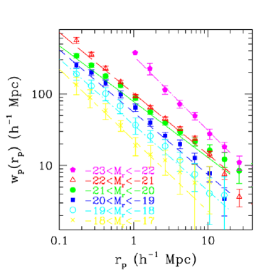
Figure 6: Luminosity-dependence of galaxy clustering. On the left is shown the projected correlation function, $w_{p}(r_{p})$, for SDSS galaxies in different absolute magnitude ranges, where brighter galaxies are seen to be more clustered. On the right is the relative bias of galaxies as a function of luminosity. Both figures are from Zehavi et al. (2005).

6.2 Color and Spectral Type Dependence

The clustering strength of galaxies also depends on restframe color and spectral type, with a stronger dependence than on luminosity. Fig. 7 shows the spatial distribution of galaxies in SDSS, color coded as a function of restframe color. Red galaxies are seen to preferentially populate the most overdense regions, while blue galaxies are more smoothly distributed in space. This is reflected in the correlation function of galaxies split by restframe color. Red galaxies have a larger correlation length and steeper slope than blue galaxies: $r_{0}$$\sim$5-6 $h^{-1}$ Mpc and $\gamma\sim$2.0 for red $L^{*}$ galaxies, while $r_{0}$$\sim$3-4 $h^{-1}$ Mpc and $\gamma\sim$1.7 for blue $L^{*}$ galaxies in SDSS (Zehavi et al., 2005). Clustering studies from the 2dFGRS split the galaxy sample at low redshift by spectral type into galaxies with emission line spectra versus absorption line spectra, corresponding to star forming and quiescent galaxies, and find similar results: that quiescent galaxies have larger correlation lengths and steeper clustering slopes than star forming galaxies (Madgwick et al., 2003).

Red and blue galaxies have distinct luminosity-dependent clustering properties. As shown in Fig. 8, the general trends seen in $r_{0}$ and $\gamma$ with luminosity for all galaxies are well-reflected in the blue galaxy population; however, at faint luminosities ($L\lesssim 0.5L^{*}$) red galaxies have larger clustering amplitudes and slopes than $L^{*}$ red galaxies. This reflects the fact that faint red galaxies are often found distributed throughout galaxy clusters.

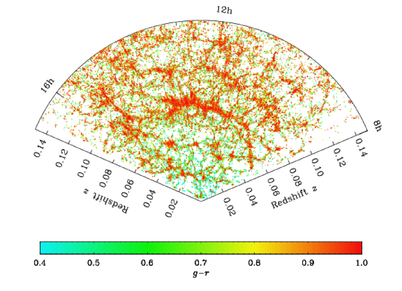
Figure 7: The spatial distribution of galaxies in the SDSS main galaxy sample as a function of redshift and right ascension, projected through 8^∘ in declination, color coded by restframe optical color. Red galaxies are seen to be more clustered than blue galaxies and generally trace the centers of groups and clusters, while blue galaxies populate further into the galaxy voids. Taken from Zehavi et al. (2011).

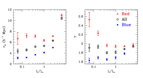
Figure 8: The clustering scale length, $r_{0}$ (left), and slope, $\gamma$ (right), for all, red, and blue galaxies in SDSS as a function of luminosity. While all galaxies are more clustered at brighter luminosities, and red galaxies are more clustered than blue galaxies at all luminosities, below $L^{*}$ the red galaxy clustering length increases at fainter luminosities. The clustering slope for faint red galaxies is also much steeper than at other luminosities. Taken from Zehavi et al. (2011).

Galaxy clustering also depends on other galaxy properties such as stellar mass, concentration index, and the strength of the 4000Å break ($D_{4000}$), in that galaxies that have larger stellar mass, more centrally concentrated light profiles, and/or larger $D_{4000}$ measurements (indicating older stellar populations) are more clustered (Li et al., 2006). This is not surprising given the observed trends with luminosity and color and the known dependencies of other galaxy properties with luminosity and color. Clearly the galaxy bias is a complicated function of various galaxy properties.

6.3 Redshift Space Distortions

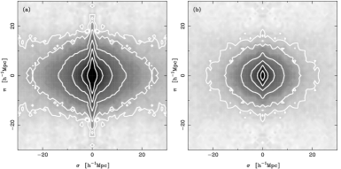
Figure 9: Two-dimensional redshift space correlation function $\xi(r_{p},\pi)$ (as in Fig. 6 here $\sigma$ is used instead of $r_{p}$) for quiescent, absorption line galaxies on the left and star forming, emission line galaxies on the right. The redshift space distortions are different for the different galaxy populations, with quiescent and/or red galaxies showing more pronounced “Fingers of God”. Both galaxy types exhibit coherent infall on large scales. Contours show lines of constant $\xi$ at $\xi=$10, 5, 2, 1, 0.5, 0.2, 0.1. Taken from Madgwick et al. (2003).

The fact that red galaxies are more clustered than blue galaxies is related to the morphology-density relation (Dressler, 1980), which results from the fact that galaxies with elliptical morphologies are more likely to be found in regions of space with a higher local surface density of galaxies. The redshift space distortions seen for red and blue galaxies also show this.

As discussed in Section 4, redshift space distortions arise from two different phenomena: virialized motions of galaxies within collapsed overdensities such as groups and clusters, and the coherent streaming motion of galaxies onto larger structures that are still collapsing. The former is seen on relatively small scales ($r_{p}\lesssim 1$ $h^{-1}$ Mpc) while the latter is detected on larger scales ($r_{P}\gtrsim 1$ $h^{-1}$ Mpc). While the presence of redshift space distortions complicates the measurement of the real space $\xi(r)$, these distortions can be used to uncover information about the thermal motions of galaxies in groups and clusters as well as the amplitude of the mass density of the Universe, $\Omega_{\rm matter}$.

Fig. 9 shows $\xi(r_{p},\pi)$ for quiescent and star forming galaxies in 2dF. The quiescent galaxies on the left show larger “Fingers of God” than the star forming galaxies on the right, reflecting the fact that red, quiescent galaxies have larger motions relative to each others. This naturally arises if red, quiescent galaxies reside in more massive, virialized overdensities with larger random peculiar velocities than star forming, optically blue galaxies. The large scale coherent infall of galaxies is seen both for blue and red galaxies, though it is often easier to see for blue galaxies, due to their smaller “Fingers of God”.

These small scale redshift space distortions can be quantified using the $\sigma_{12}$ statistic, known as the pairwise velocity dispersion (Davis et al., 1978; Fisher et al., 1994). This is measured by modeling $\xi(r_{p},\pi)$ in real space, which is then convolved with a distribution of random pairwise motions, $f(v)$, such that

$$\xi(r_{p},\pi)=\int_{-\infty}^{\infty}\xi^{\prime}(r_{p},\pi-v/H_{0})f(v)dv,$$ (23)

where the random motions are often taken to have an exponential form, which has been found to fit observed data well:

$$f(v)=\frac{1}{\sigma_{12}\sqrt{2}}\ {\rm exp}\left(-\frac{\sqrt{2}|v|}{\sigma_{12}}\right).$$ (24)

In the 2dFGRS Madgwick et al. (2003) find that $\sigma_{12}$$=416\pm 76$ km s^-1 for star forming galaxies and $\sigma_{12}$$=612\pm 92$ km s^-1 for quiescent galaxies, measured on scales of 8-20 $h^{-1}$ Mpc. Using SDSS data Zehavi et al. (2002) find that $\sigma_{12}$is $\sim 300-450$ km s^-1 for blue, star forming galaxies and $\sim 650-750$ km s^-1 for red, quiescent galaxies. It has been shown, however, that this statistic can be sensitive to large, rare overdensities, such that samples covering large volumes are needed to measures it robustly.

Madgwick et al. (2003) further measure the large scale anisotropies seen in $\xi(r_{p},\pi)$ for galaxies split by spectral type and find that $\beta=0.49\pm 0.13$ for star forming galaxies and $\beta=0.48\pm 0.14$ for quiescent galaxies. This implies a similar bias for both galaxy types on large scales, though they find that on smaller scales integrated up to 8 $h^{-1}$ Mpc, the relative bias of quiescent to star forming galaxies is $b_{rel}=1.45\pm 0.14$.

7 The Evolution of Galaxy Clustering

The observed clustering of galaxies is expected to evolve with time, as structure continues to grow due to gravity. The exact evolution depends on cosmological parameters such as $\Lambda$ and $\Omega_{\rm matter}$. Larger values of $\Lambda$, for example, lead to larger voids and higher density contrasts between overdense and underdense regions. By measuring the clustering of galaxies at higher redshift, one can break degeneracies that exist between the galaxy bias and cosmological parameters that are constrained by low redshift clustering measurements. It is therefore useful to determine the clustering of galaxies as a function of cosmic epoch, not only to further constrain cosmological parameters but also galaxy evolution.

One might expect the galaxy clustering amplitude $r_{0}$ to increase over time, as overdense regions become more overdense as galaxies move towards groups and clusters due to gravity. However, the exact evolution of the clustering of galaxies depends not only on gravity, but also on the expansion history of the Universe and therefore cosmological parameters such as $\Lambda$. Additionally, over time new galaxies form while existing galaxies grow in both mass and luminosity. Therefore, the expected changes of galaxy clustering as a function of redshift depend both on relatively well-known cosmological parameters and more unknown galaxy formation and evolution physics which likely depends on gas accretion, star formation, and feedback processes, as well as mergers.

For a given cosmological model, one can predict how the clustering of dark matter should evolve with time using cosmological N-body simulations. For a $\Lambda$CDM Universe, $r_{0}$ for dark matter particles is expected to increase from $\sim$0.8 $h^{-1}$ Mpc at $z=3$ to $\sim$5 $h^{-1}$ Mpc at $z=0$ (Weinberg et al., 2004). However, according to hierarchical structure formation theories, at high redshifts the first galaxies to form will be the first structures to collapse, which will be biased tracers of the mass. The galaxy bias is expected to be a strong function of redshift, initially $>1$ at high redshift and approaching unity over time. Therefore, $r_{0}$ for galaxies may be a much weaker function of time than it is for dark matter, as the same galaxies are not observed as a function of redshift, and over time new galaxies form in less biased locations in the Universe.

The projected angular and three dimensional correlation functions of galaxies have been observed to $z\sim 5$. Star-forming Lyman break galaxies at $z\sim 3-5$ are found to have $r_{0}$ $\sim 4-6$ $h^{-1}$ Mpc, with a bias relative to dark matter of $\sim 3-4$ (Ouchi et al., 2004; Adelberger et al., 2005). Brighter Lyman break galaxies are found to cluster more strongly than fainter Lyman break galaxies. The correlation length, $r_{0}$, is found to be roughly constant between $z=5$ and $z=3$, implying that the bias is increasing at earlier cosmic epoch. Spectroscopic galaxy surveys at $z>2$ are currently limited to samples of at most a few thousand galaxies, so most clustering measurements are angular at these epochs. In one such study by Wake et al. (2011), photometric redshifts of tens of thousands of galaxies at $1<z<2$ are used to measure the angular clustering as a function of stellar mass. They find a strong dependence of clustering amplitude on stellar mass in each of three redshift intervals in this range.

At $z\sim 1$ larger spectroscopic galaxy samples exist, and three dimensional two-point clustering analyses have been performed as a function of luminosity, color, stellar mass, and spectral type. The same general clustering trends with galaxy property that are observed at $z\sim 0$ are also seen at $z\sim 1$, in that galaxies that are brighter, redder, early spectral type, and/or more massive are more clustered. The clustering scale length of red galaxies is found to be $\sim 5-6$ $h^{-1}$ Mpc while for blue galaxies it is $\sim 3.5-4.5$ $h^{-1}$ Mpc, depending on luminosity (Meneux et al., 2006; Coil et al., 2008). At a given luminosity the observed correlation length is only $\sim$15% smaller at $z=1$ than $z=0$, indicating that unlike for dark matter the galaxy $r_{0}$ is roughly constant over time. These results are consistent with predictions from $\Lambda$CDM simulations.

The measured values of $r_{0}$ at $z\sim 1$ imply that are more biased at $z=1$ than at $z=0$. Within the DEEP2 sample, the bias measured on scales of $\sim 1-10$ $h^{-1}$ Mpc varies from $\sim 1.25-1.55$, with brighter galaxy samples being more biased tracers of the dark matter (Coil et al., 2006). These results are consistent with the idea that galaxies formed early on in the most overdense regions of space, which are biased.

As in the nearby Universe, the clustering amplitude is a stronger function of color than of luminosity at $z\sim 1$. Additionally, the color-density relation is found to already be in place at $z=1$, in that the relative bias of red to blue galaxies is as high at $z=1$ as at $z=0.1$ (Coil et al., 2008). This implies that the color-density relation is not due to cluster-specific physics, as most galaxies at $z=1$ in field spectroscopic surveys are not in clusters. Therefore it must be physical processes at play in galaxy groups that initially set the color and morphology-density relations. Red galaxies show larger “Fingers of God” in $\xi(r_{p},\pi)$ measurements than blue galaxies do, again showing that red galaxies at $z=1$ lie preferentially in virialized, more massive overdensities compared to blue galaxies. Both red and blue galaxies show coherent infall on large scales.

8 Halo Model Interpretation of $\xi(r)$

The current paradigm of galaxy formation posits that galaxies form in the center of larger dark matter halos, collapsed overdensities in the dark matter distribution with $\rho/\bar{\rho}\sim 200$, inside of which all mass is gravitationally bound. The clustering of galaxies can then be understood as a combination of the clustering of dark matter halos, which depends on cosmological parameters, and how galaxies populate dark matter halos, which depends on galaxy formation and evolution physics. For a given cosmological model the properties of dark matter halos, including their evolution with time, can be studied in detail using N-body simulations. The masses and spatial distribution of dark matter halos should depend only on the properties of dark matter, not baryonic matter, and the expansion history of the Universe; therefore the clustering of dark matter halos should be insensitive to baryon physics. However, the efficiency of galaxy formation is very dependent on the complicated baryonic physics of, for example, star formation, gas cooling, and feedback processes. The halo model allows the relatively simple cosmological dependence of galaxy clustering to be cleanly separated from the more complex baryonic astrophysics, and it shows how clustering measurements for a range of galaxy types can be used to constrain galaxy evolution physics.

8.1 Estimating the Mean Halo Mass from the Bias

One can use the observed large scale clustering amplitude of different observed galaxy populations to identify the typical mass of their parent dark matter halos, in order to place these galaxies in a cosmological context. The large scale clustering amplitude of dark matter halos as a function of halo mass is well determined in N-body simulations, and analytic fitting formula are provided by e.g., Mo & White (1996) and Sheth et al. (2001). Analytic models can then predict the clustering of both dark matter particles and galaxies as a function of scale, by using the clustering of dark matter halos and the radial density profile of dark matter and galaxies within those halos (Ma & Fry, 2000; Peacock & Smith, 2000; Seljak, 2000). In this scheme, on large, linear scales where $\delta<1$ ($\rho/\bar{\rho}\sim 1$), the clustering of a given galaxy population can be used to determine the mean mass of the dark matter halos hosting those galaxies, for a given cosmological model. To achieve this, the large-scale bias is estimated by comparing the observed galaxy clustering amplitude with that of dark matter in an N-body simulation, and then galaxies are assumed to reside in halos of a given mass that have the same bias in simulations.

Simulations show that higher mass halos cluster more strongly than lower mass halos (Sheth & Tormen, 1999). This then leads to an interpretation of galaxy clustering as a function of luminosity in which luminous galaxies reside in more massive dark matter halos than less luminous galaxies. Similarly, red galaxies typically reside in more massive halos than blue galaxies of the same luminosity; this is observationally verified by the larger “Fingers of God” observed for red galaxies. Combining the large scale bias with the observed galaxy number density further allows one to constrain the fraction of halos that host a given galaxy type, by comparing the galaxy space density to the parent dark matter halo space density. This constrains the duty cycle or fraction of halos hosting galaxies of a given population.

8.2 Halo Occupation Distribution Modeling

While such estimates of the mean host halo mass and duty cycle are fairly straightforward to carry out, a greater understanding of the relation between galaxy light and dark matter mass is gleaned by performing halo occupation distribution modeling.

The general halo-based model discussed above, in which the clustering of galaxies reflects the clustering of halos, was further developed by Peacock & Smith (2000) to include the efficiency of galaxy formation, or how galaxies populate halos. The proposed model depends on both the halo occupation number, equal to the number of galaxies in a halo of a given mass, for a galaxy sample brighter than some limit, and the location of the galaxies within these halos. In the Peacock & Smith (2000) model it is assumed that one galaxy is at the center of the halo (the “central” galaxy), and the rest of the galaxies in the same halo are “satellite” galaxies that trace the dark matter radial mass distribution, which follows an NFW profile (Navarro et al., 1997). The latter assumption results in a general power law shape for the galaxy correlation function.

A similar idea was proposed by Benson et al. (2000), who used a semi-analytic model in conjunction with a cosmological N-body simulation to show that the observed galaxy $\xi(r)$ could be reproduced with a $\Lambda$CDM  simulation (though not with a $\tau$ CDM simulation with $\Omega_{\rm matter}=1$). They also employ a method for locating galaxies inside dark matter halos such that one galaxy resides at the center of all halos above a given mass threshold, while additional galaxies are assigned the location of a random dark matter particle within the same halo, such that galaxies have the same NFW radial profile within halos as the dark matter particles (see Fig. 10, left panel).

In these models, the clustering of galaxies on scales larger than a typical halo ($\sim 1-2$ $h^{-1}$ Mpc) results from pairs of galaxies in separate halos, called the “two-halo term”, while the clustering on smaller scales ($\lesssim 1$ $h^{-1}$ Mpc) is due to pairs of galaxies within the same parent halo, called the “one-halo term”. When the pairs from these two terms are added together, the resulting galaxy correlation function should roughly follow a power law.

Benson et al. (2000) show that on large scales there is a simple relation in the bias between galaxies and dark matter halos, while on small scales the correlation function depends on the number of galaxies in a halo and the finite size of halos. When the clustering signal from these two scales (corresponding to the “two-halo” and “one-halo” terms) is combined, a power law results for the galaxy $\xi(r)$ (right panel, Fig. 10). Galaxies are found to be anti-biased relative to dark matter (i.e., less clustered than the dark matter) on scales smaller than the typical halo, though the bias is close to unity on larger scales. The clustering of galaxies that results from this semi-analytic model is also found to match the observed clustering of galaxies in the APM survey, above a given luminosity threshold (Baugh, 1996).

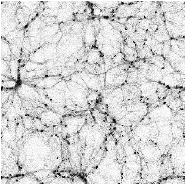
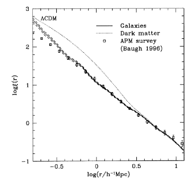
Figure 10: Left: The large scale structure seen in a $\Lambda$CDM  N-body dark matter only simulation of size 141 $\times$ 141 $\times$ 8 $h^{-3}Mpc^{3}$. The grey scale indicates the density of dark matter, while the locations of galaxies are shown with open circles. Galaxies are added to the simulation output using a semi-analytic model which assumes that dark matter halos above a given mass threshold have at least one “central” galaxy located at the center of the halo. Higher mass halos contain additional “satellite” galaxies, which are assigned the location of a random dark matter particle in the halo. Taken from Benson et al. (2000). Right: The two-point correlation function of dark matter particles (dotted line) and galaxies (solid line with dashed line showing Poisson error bars) in the simulation of Benson et al. (2000), compared with the observed clustering of galaxies in the APM survey (open squares) (Baugh, 1996).

By defining the halo occupation distribution (HOD) as the probability that a halo of a given mass contains N galaxies, $P(N|M)$, Berlind & Weinberg (2002) quantify how the observed galaxy $\xi(r)$ depends on different HOD model parameters. Using N-body simulations, they identify dark matter halos and place galaxies into the simulation using a simple HOD model with two parameters: a minimum mass at which a halo hosts, on average, one central galaxy ($M_{min}$) at the center of the halo, and the slope ($\alpha$) of the $P(N|M)$ function for satellite galaxies. The latter determines how many satellite galaxies there are as a function of halo mass. They further assume that the satellite galaxies follow an NFW profile, as the dark matter does, though the concentration of the radial profile can be changed. They show that the “two-halo term” is simply the halo center correlation function weighted by a large scale bias factor, while the “one-halo term” is sensitive to both $\alpha$ and the concentration of the galaxy profile within halos. Obtaining a power law $\xi(r)$ therefore strongly constrains the HOD model parameters.

Kravtsov et al. (2004) propose that the locations of satellite galaxies within dark matter halos should correspond to locations of subhalos, distinct gravitationally bound regions within the larger dark matter halos, instead of tracing random dark matter particles. Using cosmological N-body simulations, they show that at $z>1$ $\xi(r)$ for galaxies should deviate strongly from a power law on small scales, due to a rise in the “one-halo term”. In this model, the clustering of galaxies can be understood as the clustering of dark matter parent halos and subhalos, and the power law shape that is observed at $z\sim 0$ is a coincidence of the one- and two-halo terms having similar amplitudes and slopes at the typical scale of halos. They find that the formation and evolution of halos and subhalos through merging and dynamical processes are the main physical drivers of large scale structure.

With the unprecedentedly large galaxy sample with spectroscopic redshifts that is provided by SDSS, departures from a power law $\xi(r)$ were detected by Zehavi et al. (2004), using a volume-limited subsample of 22,000 galaxies from a parent sample of 118,000 galaxies. The deviations from a power law are small enough at $z\sim 0$ that a large sample covering a sufficiently large cosmological volume is required to overcome the errors due to cosmic variance to detect these small deviations. It is found that there is a change in the slope of $\xi(r)$ on scales of $\sim$1-2 $h^{-1}$ Mpc; this corresponds to the scale at which the one and two halo term are equal (see Fig. 11). Zehavi et al. (2004) find that $\xi(r)$ measured from the SDSS data is better fit by an HOD model, which includes small deviations from a power law, than by a pure power law. The HOD model that is fit has three parameters: the minimum mass to host a single central galaxy ($M_{\rm min}$), the minimum mass to host a single satellite galaxy ($M_{\rm 1}$), and the slope of $P(N|M)$ ($\alpha$), which determines the average number of satellite galaxies as a function of host halo mass. In this model, dark matter halos with $M_{\rm min}<M<M_{\rm 1}$ host a single galaxy, while above $M_{\rm 1}$ they host, on average, $(M/M_{\rm 1})^{\alpha}$ galaxies. Using $w_{p}(r_{p})$, one can fit for $M_{\rm 1}$ and $\alpha$, while the observed space density of galaxies is used to derive $M_{\rm min}$. For a galaxy sample with $M_{r}<-21$, the best-fit HOD parameters are $M_{\rm min}=6.1\times 10^{12}$ $h^{-1}M_{\odot}$, $M_{\rm 1}=4.7\times 10^{13}$ $h^{-1}M_{\odot}$, and $\alpha=0.89$.

Figure 11: The projected correlation function, $w_{p}(r_{p})$, for SDSS galaxies with $M_{r}<-21$ is shown as data points with error bars. The best-fit HOD model is shown as a solid line, with the contributions from the one and two halo terms shown with dotted lines. The projected correlation function of dark matter at this redshift is shown with a dashed line. The bottom panel shows deviations in $w_{p}(r_{p})$ for the data and the HOD model from the best-fit power law. Taken from Zehavi et al. (2004).

8.3 Interpreting the Luminosity and Color Dependence of Galaxy Clustering

In general, these HOD parameters reflect the efficiency of galaxy formation and evolution and can be a function of galaxy properties such as luminosity, color, stellar mass, and morphology. Zehavi et al. (2011) present HOD fits to SDSS samples as a function of luminosity and color and find that $\alpha$ is generally $\sim$1.0-1.1, though it is a bit higher for the brightest galaxies ($\sim$1.3 for $M_{r}<-22.0$). There is a strong trend between luminosity and halo mass; $M_{\rm min}$ varies as a function of luminosity from $\sim 10^{11}$ $h^{-1}M_{\odot}$ for $M_{r}<-18$ to $\sim 10^{14}$ $h^{-1}M_{\odot}$ for $M_{r}<-22$. $M_{\rm 1}$ is generally $\sim$17 times higher than the value of $M_{\rm min}$ for all luminosity threshold samples (see Fig. 12). This implies that a halo with two galaxies above a given luminosity is $\sim$17 times more massive than a halo hosting one galaxy above the same luminosity limit. Further, the fraction of galaxies that are satellites decreases at higher luminosities, from $\sim$33% at $M_{r}<-18$ to 4% at $M_{r}<-22$. The right panel of Fig. 12 shows the mass-to-light ratio of the virial halo mass to the central galaxy $r$-band luminosity as a function of halo mass. This figure shows that halos of mass $\sim 4\times 10^{11}$ $h^{-1}M_{\odot}$ are maximally efficient at galaxy formation, at converting baryons into light.

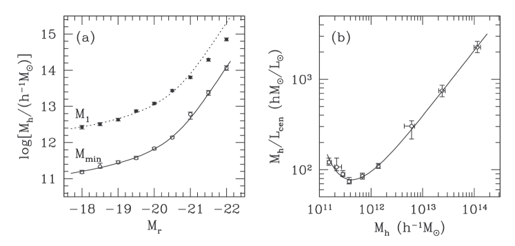
Figure 12: Left: The characteristic mass scale of dark matter halos hosting galaxies as a function of the luminosity threshold of the galaxy sample. Both the minimum halo mass to host a single galaxy is shown ($M_{\rm min}$) as well as the minimum mass to host additional satellite galaxies ($M_{\rm 1}$). A strong relationship clearly exists between halo mass and galaxy luminosity. Right: The ratio of the halo mass to the median central galaxy luminosity as a function of halo mass. Taken from Zehavi et al. (2011).

In terms of the color dependence of galaxy clustering, the trend at fainter luminosities of red galaxies being strongly clustered (with a higher correlation slope, $\gamma$, see Fig. 8) is due to faint red galaxies being satellite galaxies in relatively massive halos that host bright red central galaxies (Berlind et al., 2005). HOD modeling therefore provides a clear explanation for the increased clustering observed for faint red galaxies. For a given luminosity range $(-20<M_{r}<-19)$ Zehavi et al. (2011) fit a simplified HOD model with one parameter only to find that the fraction of galaxies that are satellites is much higher for red than for blue galaxies, with $\sim$25% of blue galaxies being satellites and $\sim$60% of red galaxies being satellites. They find that blue galaxies reside in halos with a median mass of $10^{11.7}$ $h^{-1}M_{\odot}$, while red galaxies reside in higher mass halos with a median mass of $10^{12.2}$ $h^{-1}M_{\odot}$. However, at a given luminosity, there is not a strong trend between color and halo mass (though there is a strong trend between luminosity and halo mass). Instead, the differences in $w_{p}(r_{p})$ reflect a trend between color and satellite fraction; the increased satellite fraction, in particular, drives the slope of $\xi(r)$ to be steeper for red galaxies compared to blue galaxies. And while the HOD slope $\alpha$, does not change much with increasing luminosity, it does with color, due to the dependence of the satellite fraction on color. Having a higher satellite fraction also places more galaxies in high mass halos (as those host the groups and clusters that contain the satellite galaxies), which increases the large scale bias and boosts the one halo term relative to the two halo term. The HOD model facilitates interpretion of the observed luminosity and color dependence of galaxy clustering and provides strong, crucial constraints on models of how galaxies form and evolve within their parent dark matter halos.

8.4 Interpreting the Evolution of Galaxy Clustering

As mentioned in Section 7 above, the galaxies that are observed for clustering measurements at different redshifts are not necessarily the same populations across cosmic time. A significant hurdle in understanding galaxy evolution is knowing how to connect different observed populations at different redshifts. Galaxy clustering measurements can be combined with theoretical models to trace observed populations with redshift, in that for a given cosmology one can model how the clustering of a given population should evolve with time.

The observed evolution of the luminosity-dependence of galaxy clustering can be fit surprisingly well using a simple non-parametric, non-HOD, model that relates the galaxy luminosity function to the halo mass function. Conroy et al. (2006) show that directly matching galaxies as a function of luminosity to host halos and subhalos as a function of mass leads to a model for the luminosity-dependent clustering that matches observation from $z\sim 0$ to $z\sim 3$. In this model, the only inputs are the observed galaxy luminosity function at each epoch of interest and the dark matter halo (and subhalo) mass function from N-body simulations. Galaxies are then ranked by luminosity and halos by mass and matched one-to-one, such that lower luminosity galaxies are associated with halos of lower mass, and galaxies above a given luminosity threshold are assigned to halos above a given mass threshold with the same abundance or number density. This “abundance matching” method uses as a proxy for halo mass the maximum circular velocity ($V_{\rm max}$) of the halo; for subhalos they find that it is necessary to use the value of $V_{\rm max}$ when the subhalo is first accreted into a larger halo, to avoid the effects of tidal stripping. With this simple model the clustering amplitude and shape as a function of luminosity are matched for SDSS galaxies at $z\sim 0$, DEEP2 galaxies at $z\sim 1$, and Lyman break galaxies at $z\sim 3$. In particular, the clustering amplitude in both the one and two halo regimes is well fit, including the deviations from a power law that seen at $z>1$ (Ouchi et al., 2005; Coil et al., 2006). These results imply a tight correlation between galaxy luminosity and halo mass from $z\sim 0$ to $z\sim 3$.

While abundance-matching techniques provide a simple, zero parameter model for how galaxies populate halos, a richer understanding of the physical properties involved may be gained by performing HOD modeling. Zheng et al. (2007) use HOD modeling to fit the observed luminosity-dependent galaxy clustering at $z\sim 0$ measured in SDSS with that measured at $z\sim 1$ in DEEP2 to confirm that at both epochs there is a tight relationship between the central galaxy luminosity and host halo mass. At $z\sim 1$ the satellite fraction drops for higher luminosities, as at $z\sim 0$, but at a given luminosity the satellite fraction is higher at $z\sim 0$ than at $z\sim 1$. They also find that at a given central luminosity, halos are $\sim$1.6 times more massive at $z\sim 0$ than $z\sim 1$, and at a given halo mass galaxies are $\sim$1.4 times more luminous at $z\sim 1$ than $z\sim 0$.

Zheng et al. (2007) further combine these HOD results with theoretical predictions of the growth of dark matter halos from simulations to link $z\sim 1$ central galaxies to their descendants at $z\sim 0$ and find that the growth of both halo mass and stellar mass as a function of redshift depends on halo mass. Lower mass halos grow earlier, which is reflected in the fact that more of their $z\sim 0$ mass is already assembled by $z\sim 1$. A typical $z\sim 0$ halo with mass $3\times 10^{11}$ $h^{-1}M_{\odot}$ has about 70% of its final mass in place by $z\sim 1$, while a $z\sim 0$ halo with mass $10^{13}$ $h^{-1}M_{\odot}$ has $\sim$50% of its final mass in place at $z\sim 1$. In terms of stellar mass, however, in a $z\sim 0$ halo of mass $5\times 10^{11}$ $h^{-1}M_{\odot}$ a central galaxy has $\sim$20% of its stellar mass in place at $z\sim 1$, while the fraction rises to $\sim$33% above a halo mass of $2\times 10^{12}$ $h^{-1}M_{\odot}$. They further find that the mass scale of the maximum star formation efficiency for central galaxies shifts to lower halo mass with time, with a peak of $\sim 10^{12}$ $h^{-1}M_{\odot}$ at $z\sim 1$ and $\sim 6\times 10^{11}$ $h^{-1}M_{\odot}$at $z\sim 0$.

At $1<z<2$, Wake et al. (2011) use precise photometric redshifts from the NEWFIRM survey to measure the relationship between stellar mass and dark matter halo mass using HOD models. At these higher redshifts $r_{0}$ varies from $\sim$6 to $\sim$11 $h^{-1}$ Mpc for stellar masses $\sim 10^{10}$ $M_{\odot}$ to $10^{11}$ $M_{\odot}$. The galaxy bias is a function of both redshift and stellar mass and is $\sim$2.5 at $z\sim 1$ and increases to $\sim$3.5 at $z\sim 2$. They find that the typical halo mass of both central and satellite galaxies increases with stellar mass, while the satellite fraction drops at higher stellar mass, qualitatively similar to what is found at lower redshift. They do not find evolution in the relationship between stellar mass and halo mass between $z\sim 2$ and $z\sim 1$, but do find evolution compared to $z\sim 0$. They also find that the peak of star formation efficiency shifts to lower halo mass with time.

Simulations can also be used to connect different observed galaxy populations at different redshifts. An example of the power of this method is shown by Conroy et al. (2008), who compare the clustering and space density of star forming galaxies at $z\sim 2$ with that of star forming and quiescent galaxies at $z=1$ and $z=0$ to infer both the typical descendants of the $z\sim 2$ star forming galaxies and constrain the fraction that have merged with other galaxies by $z=0$. They use halos and subhalos identified in a $\Lambda$CDM  N-body simulation to determine which halos at $z\sim 2$ likely host star forming galaxies, and then use the merger histories in the simulation to track these same halos to lower redshift. By comparing these results to observed clustering of star forming galaxies at $z\sim 1$ and $z\sim 0$ they can identify the galaxy populations at these epochs that are consistent with being descendants of the $z\sim 2$ galaxies. They find that while the lower redshift descendent halos have clustering strengths similar to red galaxies at both $z\sim 1$ and $z\sim 0$, the $z\sim 2$ star forming galaxies can not all evolve into red galaxies by lower redshift, as their space density is too high. There are many more lower redshift descendents than there are red galaxies, even after taking into account mergers. They conclude that most $z\sim 2$ star forming galaxies evolve into typical $L^{*}$ galaxies today, while a non-negligible fraction become satellite galaxies in larger galaxy groups and clusters.

In summary, N-body simulations and HOD modeling can be used to interpret the observed evolution of galaxy clustering and further constrain both cosmological parameters and theoretical models of galaxy evolution beyond what can be gleaned from $z\sim 0$ observations alone. They also establish links between distinct observed galaxy populations at different redshifts, allowing one to create a coherent picture of how galaxies evolve over cosmic time.

9 Voids and Filaments

Redshift surveys unveil a rich structure of galaxies, as seen in Fig. 3. In addition to measuring the two-point correlation function to quantify the clustering amplitude as a function of galaxy properties, one can also study higher-order clustering measurements as well as properties of voids and filaments.

9.1 Higher-order Clustering Measurements

Higher-order clustering statistics reflect both the growth of initial density fluctuations as well as the details of galaxy biasing (Bernardeau et al., 2002), such that measurements of higher-order clustering can test the paradigm of structure formation through gravitational instability as well as constrain the galaxy bias. In the linear regime there is a degeneracy between the amplitude of fluctuations in the dark matter density field and the galaxy bias, in that a highly clustered galaxy population may be biased and trace only the most overdense regions of the dark matter, or the dark matter itself may be highly clustered. However, this degeneracy can be broken in the non-linear regime on small scales. Over time, the density field becomes skewed towards high density as $\delta$ becomes greater than unity in overdense regions (where $\delta\equiv(\rho/\bar{\rho})-1$ ) but can not become negative in underdense regions. Skewness in the galaxy density distribution can also arise from galaxy bias, if galaxies preferentially form in the highest density peaks. One can therefore use the shapes of the galaxy overdensities, through measurements of the three-point correlation function, to test gravitational collapse versus galaxy bias.

To study higher-order clustering one needs large samples that cover enormous volumes; all studies to date have focused on low redshift galaxies. Verde et al. (2002) use 2dFGRS to measure the Fourier transform of the three-point correlation function, called the bispectrum, to constrain the galaxy bias without resorting to comparisons with N-body simulations in order to measure the clustering of dark matter. Fry & Gaztanaga (1993) present the galaxy bias in terms of a Taylor expansion of the density contrast, where the first order term is the linear term, while the second order term is the non-linear or quadratic term. Measured on scales of 5 – 30 $h^{-1}$ Mpc, Verde et al. (2002) find that the linear galaxy bias is consistent with unity ($b_{1}=1.04\pm 0.11$), while the non-linear quadratic bias is consistent with zero ($b_{2}=-0.05\pm 0.08$). When combined with the redshift space distortions measured in the two-dimensional two-point correlation function ($\xi(r_{p},\pi)$), they measure $\Omega_{\rm matter}=0.27\pm 0.06$ at $z=0.17$. This constraint on the matter density of the Universe is derived entirely from large scale structure data alone.

Gaztañaga et al. (2005) measure the three-point correlation function in 2dFGRS for triangles of galaxy configurations with different shapes. Their results are consistent with $\Lambda$CDM expectations regarding gravitational instability of initial Gaussian fluctuations. Furthermore, they find that while the linear bias is consistent with unity ($b_{1}=0.93+0.10/-0.08$), the quadratic bias is non-zero ($b_{2}/b_{1}=-0.34+0.11/-0.08$). This implies that there is a non-gravitational contribution to the three-point function, resulting from galaxy formation physics. These results differ from those of Verde et al. (2002), which may be due to the inclusion by Gaztañaga et al. (2005) of the covariance between measurements on different scales. Gaztañaga et al. (2005) combine their results with the measured two-point correlation function to derive $\sigma_{8}=0.88+0.12/-0.10$.

If the density field follows a Gaussian distribution, the higher-order clustering terms can be expressed solely in terms of the lower order clustering terms. This “hierarchical scaling” holds for the evolution of an initially Gaussian distribution of fluctuations under gravitational instability. Therefore departures from hierarchical scaling can result either from a non-Gaussian initial density field or from galaxy bias. Redshift space higher-order clustering measurements in 2dFGRS are performed by Baugh et al. (2004) and Croton et al. (2004a), who measure up to the six-point correlation function. They find that hierarchical scaling is obeyed on small scales, though deviations exist on larger scales ($\sim 10$ $h^{-1}$ Mpc). They show that on large scales the higher-order terms can be significantly affected by massive rare peaks such as superclusters, which populate the tail of the overdensity distribution. Croton et al. (2004a) also show that the three-point function has a weak luminosity dependence, implying that galaxy bias is not entirely linear. These results are confirmed by Nichol et al. (2006) using galaxies in the SDSS, who also measure a weak luminosity dependence in the three-point function. They find that on scales $>$10 $h^{-1}$ Mpc the three-point function is greatly affected by the “Sloan Great Wall”, a massive supercluster that is roughly 450 Mpc (Gott et al., 2005) in length and is associated with tens of known Abell clusters. These results show that even 2dFGRS and SDSS are not large enough samples to be unaffected by the most massive, rare structures.

Several studies have examined higher-order correlation functions for galaxies split by color. Gaztañaga et al. (2005) find a strong dependence of the three-point function on color and luminosity on scales $<$6 $h^{-1}$ Mpc. Croton et al. (2007) measure up to the five-point correlation function in 2dFGRS for both blue and red galaxies and find that red galaxies are more clustered than blue galaxies in all of the N-point functions measured. They also find a luminosity-dependence in the hierarchical scaling amplitudes for red galaxies but not for blue galaxies. Taken together, these results explain why the full galaxy population shows only a weak correlation with luminosity.

9.2 Voids

In maps of the large scale structure of galaxies, voids stand out starkly to the eye. There appear to be vast regions of space with few, if any, $L^{*}$ galaxies. Voids are among the largest structures observed in the Universe, spanning typically tens of $h^{-1}$ Mpc.

The statistics of voids – their sizes, distribution, and underdensities – are closely tied to cosmological parameters and the physical details of structure formation (e.g. Sheth & van de Weygaert (2004)). While the two-point correlation function provides a full description of clustering for a Gaussian distribution, departures from Gaussianity can be tested with higher-order correlation statistics and voids. For example, the abundance of voids can be used to test the non-Gaussianity of primordial perturbations, which constrains models of inflation (Kamionkowski et al., 2009). Additionally, voids provide an extreme low density environment in which to study galaxy evolution. As discussed by Peebles (2001), the lack of galaxies in voids should provide a stringent test for galaxy formation models.

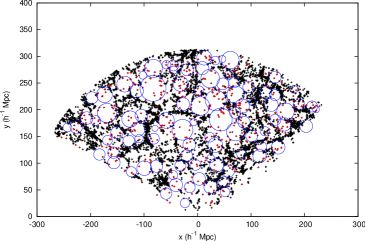
Figure 13: Void and wall galaxies in the SDSS. Shown is a projection of a 10 $h^{-1}$ Mpc slab with wall galaxies plotted as black crosses and void galaxies plotted as red crosses. Blue circles indicate the intersection of the maximal sphere of each void with the midplane of the slab (from Pan et al. 2011).

9.2.1 Void and Void Galaxy Properties

The first challenge in measuring the properties of voids and void galaxies is defining the physical extent of individual voids and identifying which galaxies are likely to be in voids. The “void finder” algorithm of El-Ad & Piran (1997), which is based on the point distribution of galaxies (i.e., does not perform any smoothing), is widely used. This algorithm does not assume that voids are entirely devoid of galaxies and identifies void galaxies as those with three or less neighboring galaxies within a sphere defined by the mean and standard deviation of the distance to the third nearest neighbor for all galaxies. All other galaxies are termed “wall” galaxies. An individual void is then identified as the maximal sphere that contains only void galaxies (see Fig. 10). This algorithm is widely used by both theorists and observers.

Cosmological simulations of structure formation show that the distribution and density of galaxy voids are sensitive to the values of $\Omega_{\rm matter}$ and $\Omega_{\rm\Lambda}$ (Kauffmann et al., 1999). Using $\Lambda$CDM N-body dark matter simulations, Colberg et al. (2005) study the properties of voids within the dark matter distribution and predicts that voids are very underdense (though not empty) up to a well-defined, sharp edge in the dark matter density. They predict that 61% of the volume of space should be filled by voids at $z=0$, compared to 28% at $z=1$ and 9% at $z=2$. They also find that the mass function of dark matter halos in voids is steeper than in denser regions of space.

Using similar $\Lambda$CDM N-body simulations with a semi-analytic model for galaxy evolution, Benson et al. (2003) show that voids should contain both dark matter and galaxies, and that the dark matter halos in voids tend to be low mass and therefore contain fewer galaxies than in higher density regions. In particular, at density contrasts of $\delta<-0.6$, where $\delta\equiv(\rho/\rho_{\rm mean})-1$, both dark matter halos and galaxies in voids should be anti-biased relative to dark matter. However, galaxies are predicted to be more underdense than the dark matter halos, assuming simple physically-motivate prescriptions for galaxy evolution. They also predict the statistical size distribution of voids, finding that there should be more voids with smaller radii ($<10$$h^{-1}$ Mpc) than larger radii.

The advent of the 2dFGRS and SDSS provided the first very large samples of voids and void galaxies that could be used to robustly measure their statistical properties. Applying the ”void finder” algorithm on the 2dFGRS dataset, Hoyle & Vogeley (2004) find that the typical radius of voids is $\sim$15 $h^{-1}$ Mpc. Voids are extremely underdense, with an average density of $\delta\rho/\rho$=-0.94, with even lower densities at the center, where fewer galaxies lie. The volume of space filled by voids is $\sim$40%. Probing an even larger volume of space using the SDSS dataset, Pan et al. (2011) find a similar typical void radius and conclude that $\sim$60% of space is filled by voids, which have $\delta\rho/\rho$=-0.85 at their edges. Voids have sharp density profiles, in that they remain extremely underdense to the void radius, where the galaxy density rises steeply. These observational results agree well with the predictions of $\Lambda$CDM simulations discussed above.

Studies of the properties of galaxy in voids allow an understanding of how galaxy formation and evolution progresses in the lowest density environments in the Universe, effectively pursuing the other end of the density spectrum from cluster galaxies. Void galaxies are found to be significantly bluer and fainter than wall galaxies (Rojas et al., 2004). The luminosity function of void galaxies shows a lack of bright galaxies but no difference in the measured faint end slope (Croton et al., 2005; Hoyle et al., 2005), indicating that dwarf galaxies are not likely to be more common in voids. The normalization of the luminosity function of wall galaxies is roughly an order of magnitude higher than that of void galaxies; therefore galaxies do exist in voids, just with a much lower space density. Studies of the optical spectra of void galaxies show that they have high star formation rates, low 4000Å spectral breaks indicative of young stellar populations, and low stellar masses, resulting in high specific star formation rates (Rojas et al., 2005).

However, red quiescent galaxies do exist in voids, just with a lower space density than blue, star forming galaxies (Croton et al., 2005). Croton & Farrar (2008) show that the observed luminosity function of void galaxies can be replicated with a $\Lambda$CDM N-body simulation and simple semi-analytic prescriptions for galaxy evolution. They explain the existence of red galaxies in voids as residing in the few massive dark matter halos that exist in voids. Their model requires some form of star formation quenching in massive halos ($>\sim 10^{12}$ $M_{\odot}$), but no additional physics that operates only at low density needs to be included in their model to match the data. It is therefore the shift in the halo mass function in voids that leads to different galaxy properties, not a change in the galaxy evolution physics in low density environments.

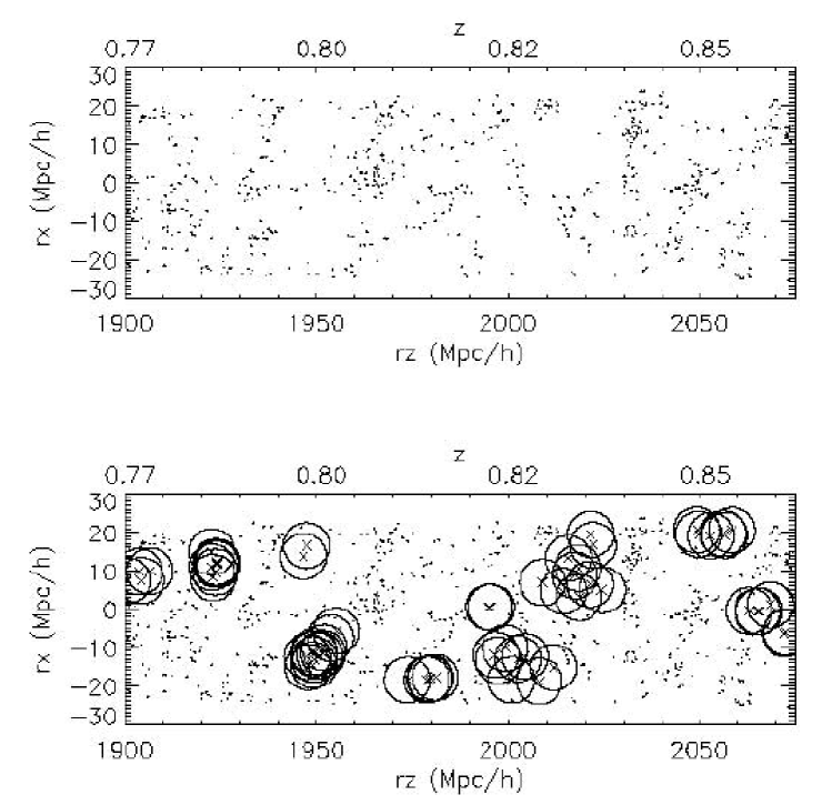
Figure 14: A schematic of the void probability function (VPF). The top panel shows the comoving distribution of galaxies in a small portion of the DEEP2 survey (projected through 10 $h^{-1}$ Mpc), while the lower panel shows a fraction of the empty spheres identified with a radius of 6 $h^{-1}$ Mpc in the same volume (from Conroy et al. 2005). Because the figure is projected through one dimension, it may appear that galaxies reside inside of identified voids; in three dimensions the voids contain no galaxies.

9.2.2 Void Probability Function

In addition to identifying individual voids and the galaxies in them, one can study the statistical distribution of voids using the void probability function (VPF). Defined by White (1979), the VPF is the probability that a randomly placed sphere of radius $R$ within a point distribution will not contain any points (i.e., galaxies, see Figure 11). The VPF is defined such that it depends on the space density of points; therefore one must be careful when comparing datasets and simulation results to ensure that the same number density is used. The VPF traces clustering in the weakly non-linear regime, not in the highly non-linear regime of galaxy groups and clusters.

Benson et al. (2003) predict using $\Lambda$CDM simulations that the VPF of galaxies should be higher than that of dark matter, that voids as traced by galaxies are much larger than voids traced by dark matter. This results from the bias of galaxies compared to dark matter in voids and the fact that in this model the few dark matter halos that do exist in voids are low mass and therefore often do not contain bright galaxies. Croton et al. (2004b) measure the VPF in the 2dFGRS dataset and find that it follows hierarchical scaling laws, in that all higher-order correlation functions can be expressed in terms of the two-point correlation function. They find that even on scales of $\sim$30 $h^{-1}$ Mpc, higher-order correlations have an impact, and that the VPF of galaxies is observed to be different than that of dark matter in simulations.

Conroy et al. (2005) measure the VPF in SDSS galaxies at $z\sim 0.1$ and DEEP2 galaxies at $z\sim 1$ and find that voids traced by redder and/or brighter galaxy populations are larger than voids traced by bluer and/or fainter galaxies. They also find that voids are larger in comoving coordinates at $z\sim 0.1$ than at $z\sim 1$; i.e., voids grow over time, as expected. They show that the differences observed in the VPF as traced by different galaxy populations are entirely consistent with differences observed in the two-point correlation function and space density of these galaxy populations. This implies that there does not appear to be additional higher-order information in voids than in the two-point function alone. They also find excellent agreement with predictions from $\Lambda$CDM simulations that include semi-analytic models of galaxy evolution.

Tinker et al. (2008) interpret the observed VPF in galaxy surveys in terms of the halo model (see Section 8 above). They compare the observed VPF in 2dFGRS and SDSS to halo model predictions constrained to match the two-point correlation function and number density of galaxies, using a model in which the dark matter halo occupation depends on mass only. They find that with this model they can match the observed data very well, implying that there is no need for the suppression of galaxy formation in voids; i.e., galaxy formation does not proceed differently in low-density regions. They find that the sizes and emptiness of voids show excellent agreement with predictions of $\Lambda$CDM models for galaxies at low redshift to luminosities of $L\sim 0.2L^{*}$.

9.3 Filaments

Galaxy filaments – long strings of galaxies – are the largest systems seen in maps of large scale structure, and as such provide a key test of theories of structure formation. Aragón-Calvo et al. (2010) show that in simulations while filaments occupy only $\sim 10$% of the volume of space, they account for $\sim$40% of the mass content of the $z=0$ Universe. Measuring the typical and maximal length of filaments, as well as their thickness and average density, therefore constrains theoretical models. Various statistical methods have been proposed to identify and characterize the morphologies and properties of filaments (e.g. Sousbie et al. (2008) and references therein).

In terms of their sizes, the largest length scale at which filaments are statistically significant, and hence identified as real objects, is 50-80 $h^{-1}$ Mpc, according to an analysis of galaxies in the Las Campanas Redshift Survey (LCRS; Shectman et al., 1996) by Bharadwaj et al. (2004). They show that while there appear to be filaments in the survey on longer scales, these arise from chance alignments and projection effects and are not real structures. Sousbie et al. (2008) identify and study the length of filaments in SDSS, by identifying ridges in the galaxy distribution using the Hessian matrix ($\partial^{2}\rho/\partial x_{i}\partial x_{j}$) and its eigenvalues (see Fig. 12). They find excellent agreement between observations and $\Lambda$CDM numerical predictions for a flat, low $\Omega_{\rm matter}$ Universe. They argue that filament measurements are not highly sensitive to observational effects such as redshift space distortions, edge effects, incompleteness or galaxy bias, which makes them a robust test of theoretical models.

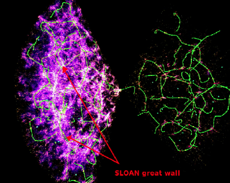
Figure 15: Filaments identified in the SDSS galaxy distribution (from Sousbie et al. 2008). Individual filaments are shown in green overlaid on the galaxy density field show in purple. The Sloan Great Wall is identified in the foreground, lying between the red arrows.

Bond et al. (2010) use the eigenvectors of the Hessian matrix of the smoothed galaxy distribution to identify filaments in both SDSS data and $\Lambda$CDM simulations and find that the distribution of filaments lengths is roughly exponential, with many more filaments of length $\lesssim$10 $h^{-1}$ Mpc than $>20$ $h^{-1}$ Mpc. They find that the filament width distribution agrees between the SDSS data and N-body simulations. The mean filament width depends on the smoothing length; for smoothing scales of 10 and $h^{-1}$ Mpc, the mean filament widths are 5.5 and 8.4 $h^{-1}$ Mpc. In $\Lambda$CDM simulations they find that the filamentary structure in the dark matter density distribution is in place by $z=3$, tracing a similar pattern of density ridges. This is in contrast to what is found for voids, which become much more prominent and low-density at later cosmic epochs.

Choi et al. (2010) use the methods of Bond et al. (2010) to study the evolution of filamentary structure from $z\sim 0.8$ to $z\sim 0.1$ using galaxies from the DEEP2 survey and the SDSS. They find that neither the space density of filaments nor the distribution of filament lengths has changed significantly over the last seven Gyr of cosmic time, in agreement with $\Lambda$CDM numerical predictions. The distribution of filament widths has changed, however, in that the distribution is broader at lower redshift and has a smaller typical width. This observed evolution in the filament width distribution naturally results from non-linear growth of structure and is consistent with the results on voids discussed above, in that over time voids grow larger while filaments become tighter (i.e. have a smaller typical width) though not necessarily longer.

10 Summary and Future

This overview of our current understanding of the large-scale structure of the Universe has shown that quantitative measurements of the clustering and spatial distribution of galaxies have wide applications and implications. The non-uniform structure reveals properties of both the galaxies and the dark matter halos that comprise this large-scale structure. Statistics such as the two-point correlation function can be used not only to constrain cosmological parameters but also to understand galaxy formation and evolution processes. The advent of extremely large redshift surveys with samples of hundreds of thousands of galaxies has led to very precise measurements of the clustering of galaxies at $z\sim 0.1$ as a function of various galaxy properties such as luminosity, color, and stellar mass, influencing our understanding of how galaxies form and evolve. Initial studies at higher redshift have revealed that many of the general correlations that are observed between galaxy properties and clustering at $z\sim 0$ were in place when the Universe was a fraction of its current age. As larger redshift surveys are carried out at higher redshifts, much more can be learned about how galaxy populations change with time. Theoretical interpretations of galaxy clustering measurements such as the halo occupation distribution model have also recently made great strides in terms of statistically linking various properties of galaxies with those of their host dark matter halos. Such studies reveal not only how light traces mass on large scales but how baryonic mass and dark matter co-evolve with cosmic time.

There are many exciting future directions for studies of galaxy clustering and large-scale structure. Precise cosmological constraints can be obtained using baryon acoustic oscillation signatures observed in clustering measurements from wide-area surveys (Eisenstein et al., 2005). Specific galaxy populations can be understood in greater detail by comparing their clustering properties with those of galaxies in general. For example, the clustering of different types of active galactic nuclei (AGN) can be used to constrain the AGN fueling mechanisms, lifetimes, and host galaxy populations (Coil et al., 2009). As discussed above, measurements of galaxy clustering have the power to place strong constraints on contemporary models of galaxy formation and evolution and advance our understanding of how galaxies populate and evolve within dark matter halos.

The author thanks James Aird, Mirko Krumpe, and Stephen Smith for providing comments on earlier drafts of the text.

References

- Adelberger et al. (2005) Adelberger, K. L., et al. 2005, ApJ, 619, 697
- Aragón-Calvo et al. (2010) Aragón-Calvo, M. A., van de Weygaert, R., & Jones, B. J. T. 2010, MNRAS, 408, 2163
- Bardeen et al. (1986) Bardeen, J. M., Bond, J. R., Kaiser, N., & Szalay, A. S. 1986, ApJ, 304, 15
- Baugh (1996) Baugh, C. M. 1996, MNRAS, 280, 267
- Baugh et al. (2004) Baugh, C. M., et al. 2004, MNRAS, 351, L44
- Benson et al. (2000) Benson, A. J., Cole, S., Frenk, C. S., Baugh, C. M., & Lacey, C. G. 2000, MNRAS, 311, 793
- Benson et al. (2003) Benson, A. J., Hoyle, F., Torres, F., & Vogeley, M. S. 2003, MNRAS, 340, 160
- Berlind & Weinberg (2002) Berlind, A. A., & Weinberg, D. H. 2002, ApJ, 575, 587
- Berlind et al. (2005) Berlind, A. A., et al. 2005, ApJ, 629, 625
- Bernardeau et al. (2002) Bernardeau, F., Colombi, S., Gaztañaga, E., & Scoccimarro, R. 2002, PhR, 367, 1
- Bharadwaj et al. (2004) Bharadwaj, S., Bhavsar, S. P., & Sheth, J. V. 2004, ApJ, 606, 25
- Bond et al. (2010) Bond, N. A., Strauss, M. A., & Cen, R. 2010, MNRAS, 409, 156
- Brodwin et al. (2008) Brodwin, M., et al. 2008, ApJL, 687, L65
- Choi et al. (2010) Choi, E., et al. 2010, MNRAS, 406, 320
- Coil et al. (2006) Coil, A. L., et al. 2006, ApJ, 644, 671
- Coil et al. (2008) —. 2008, ApJ, 672, 153
- Coil et al. (2009) —. 2009, ApJ, 701, 1484
- Colberg et al. (2005) Colberg, J. M., et al. 2005, MNRAS, 360, 216
- Colless et al. (2001) Colless, M., et al. 2001, MNRAS, 328, 1039
- Conroy et al. (2006) Conroy, C., Wechsler, R. H., & Kravtsov, A. V. 2006, ApJ, 647, 201
- Conroy et al. (2005) Conroy, C., et al. 2005, ApJ, 635, 990
- Conroy et al. (2008) —. 2008, ApJ, 679, 1192
- Croton & Farrar (2008) Croton, D. J., & Farrar, G. R. 2008, MNRAS, 386, 2285
- Croton et al. (2007) Croton, D. J., Norberg, P., Gaztañaga, E., & Baugh, C. M. 2007, MNRAS, 379, 1562
- Croton et al. (2004a) Croton, D. J., et al. 2004a, MNRAS, 352, 1232
- Croton et al. (2004b) —. 2004b, MNRAS, 352, 828
- Croton et al. (2005) —. 2005, MNRAS, 356, 1155
- Davis et al. (1978) Davis, M., Geller, M. J., & Huchra, J. 1978, ApJ, 221, 1
- Davis et al. (1982) Davis, M., Huchra, J., Latham, D. W., & Tonry, J. 1982, ApJ, 253, 423
- Davis & Peebles (1983) Davis, M., & Peebles, P. J. E. 1983, ApJ, 267, 465
- Dressler (1980) Dressler, A. 1980, ApJ, 236, 351
- Eisenstein et al. (2005) Eisenstein, D. J., et al. 2005, ApJ, 633, 560
- El-Ad & Piran (1997) El-Ad, H., & Piran, T. 1997, ApJ, 491, 421
- Fisher et al. (1994) Fisher, K. B., Davis, M., Strauss, M. A., Yahil, A., & Huchra, J. P. 1994, MNRAS, 267, 927
- Fry (1996) Fry, J. N. 1996, ApJL, 461, L65
- Fry & Gaztanaga (1993) Fry, J. N., & Gaztanaga, E. 1993, ApJ, 413, 447
- Gaztañaga et al. (2005) Gaztañaga, E., Norberg, P., Baugh, C. M., & Croton, D. J. 2005, MNRAS, 364, 620
- Geller & Huchra (1989) Geller, M. J., & Huchra, J. P. 1989, Science, 246, 897
- Gott et al. (1986) Gott, III, J. R., Dickinson, M., & Melott, A. L. 1986, ApJ, 306, 341
- Gott et al. (2005) Gott, III, J. R., et al. 2005, ApJ, 624, 463
- Gregory & Thompson (1978) Gregory, S. A., & Thompson, L. A. 1978, ApJ, 222, 784
- Guzzo et al. (2008) Guzzo, L., et al. 2008, Nature, 451, 541
- Hamilton (1992) Hamilton, A. J. S. 1992, ApJL, 385, L5
- Hamilton (1993) —. 1993, ApJ, 417, 19
- Hamilton (1998) Hamilton, A. J. S. 1998, in ASSL Vol. 231: The Evolving Universe, 185
- Hoyle et al. (2005) Hoyle, F., Rojas, R. R., Vogeley, M. S., & Brinkmann, J. 2005, ApJ, 620, 618
- Hoyle & Vogeley (2004) Hoyle, F., & Vogeley, M. S. 2004, ApJ, 607, 751
- Hubble (1934) Hubble, E. 1934, ApJ, 79, 8
- Hubble (1926) Hubble, E. P. 1926, ApJ, 64, 321
- Joeveer et al. (1978) Joeveer, M., Einasto, J., & Tago, E. 1978, MNRAS, 185, 357
- Kaiser (1984) Kaiser, N. 1984, ApJL, 284, L9
- Kaiser (1987) —. 1987, MNRAS, 227, 1
- Kamionkowski et al. (2009) Kamionkowski, M., Verde, L., & Jimenez, R. 2009, JCAP, 1, 10
- Kauffmann et al. (1999) Kauffmann, G., Colberg, J. M., Diaferio, A., & White, S. D. M. 1999, MNRAS, 303, 188
- Kerscher et al. (2000) Kerscher, M., Szapudi, I., & Szalay, A. S. 2000, ApJL, 535, L13
- Kirshner et al. (1978) Kirshner, R. P., Oemler, Jr., A., & Schechter, P. L. 1978, AJ, 83, 1549
- Kravtsov et al. (2004) Kravtsov, A. V., et al. 2004, ApJ, 609, 35
- Landy & Szalay (1993) Landy, S. D., & Szalay, A. S. 1993, ApJ, 412, 64
- Li et al. (2006) Li, C., et al. 2006, MNRAS, 368, 21
- Ma & Fry (2000) Ma, C.-P., & Fry, J. N. 2000, ApJ, 543, 503
- Maddox et al. (2010) Maddox, S. J., et al. 2010, A&A, 518, L11
- Madgwick et al. (2003) Madgwick, D. S., et al. 2003, MNRAS, 344, 847
- Mann et al. (1998) Mann, R. G., Peacock, J. A., & Heavens, A. F. 1998, MNRAS, 293, 209
- Meneux et al. (2006) Meneux, B., et al. 2006, A&A, 452, 387
- Mo & White (1996) Mo, H. J., & White, S. D. M. 1996, MNRAS, 282, 347
- Navarro et al. (1997) Navarro, J. F., Frenk, C. S., & White, S. D. M. 1997, ApJ, 490, 493
- Nichol et al. (2006) Nichol, R. C., et al. 2006, MNRAS, 368, 1507
- Norberg et al. (2001) Norberg, P., et al. 2001, MNRAS, 328, 64
- Ouchi et al. (2004) Ouchi, M., et al. 2004, ApJ, 611, 685
- Ouchi et al. (2005) —. 2005, ApJL, 635, L117
- Pan et al. (2011) Pan, D. C., Vogeley, M. S., Hoyle, F., Choi, Y.-Y., & Park, C. 2011, ArXiv e-prints
- Peacock & Smith (2000) Peacock, J. A., & Smith, R. E. 2000, MNRAS, 318, 1144
- Peacock et al. (2001) Peacock, J. A., et al. 2001, Nature, 410, 169
- Peebles (1975) Peebles, P. J. E. 1975, ApJ, 196, 647
- Peebles (1980) —. 1980, The Large-Scale Structure of the Universe (Princeton, N.J., Princeton Univ. Press)
- Peebles (2001) —. 2001, ApJ, 557, 495
- Postman et al. (1998) Postman, M., Lauer, T. R., Szapudi, I., & Oegerle, W. 1998, ApJ, 506, 33
- Roche & Eales (1999) Roche, N., & Eales, S. A. 1999, MNRAS, 307, 703
- Rojas et al. (2004) Rojas, R. R., Vogeley, M. S., Hoyle, F., & Brinkmann, J. 2004, ApJ, 617, 50
- Rojas et al. (2005) —. 2005, ApJ, 624, 571
- Sandage & Tammann (1975) Sandage, A., & Tammann, G. A. 1975, ApJ, 196, 313
- Sargent & Turner (1977) Sargent, W. L. W., & Turner, E. L. 1977, ApJL, 212, L3
- Scoccimarro (2000) Scoccimarro, R. . 2000, ApJ, 544, 597
- Seldner et al. (1977) Seldner, M., Siebers, B., Groth, E. J., & Peebles, P. J. E. 1977, AJ, 82, 249
- Seljak (2000) Seljak, U. 2000, MNRAS, 318, 203
- Shane & Wirtanen (1967) Shane, C. D., & Wirtanen, C. A. 1967, in Pub. Lick Obs. Vol. 22, part 1
- Shapley & Ames (1932) Shapley, H., & Ames, A. 1932, Annals of Harvard College Observatory, 88, 41
- Shectman et al. (1996) Shectman, S. A., et al. 1996, ApJ, 470, 172
- Sheth et al. (2001) Sheth, R. K., Mo, H. J., & Tormen, G. 2001, MNRAS, 323, 1
- Sheth & Tormen (1999) Sheth, R. K., & Tormen, G. 1999, MNRAS, 308, 119
- Sheth & van de Weygaert (2004) Sheth, R. K., & van de Weygaert, R. 2004, MNRAS, 350, 517
- Sousbie et al. (2008) Sousbie, T., et al. 2008, ApJL, 672, L1
- Tegmark & Peebles (1998) Tegmark, M., & Peebles, P. J. E. 1998, ApJL, 500, L79
- Tegmark et al. (2004) Tegmark, M., et al. 2004, ApJ, 606, 702
- Tinker et al. (2008) Tinker, J. L., et al. 2008, ApJ, 686, 53
- Verde et al. (2002) Verde, L., et al. 2002, MNRAS, 335, 432
- Wake et al. (2011) Wake, D. A., et al. 2011, ApJ, 728, 46
- Weinberg et al. (2004) Weinberg, D. H., Davé, R., Katz, N., & Hernquist, L. 2004, ApJ, 601, 1
- White (1979) White, S. D. M. 1979, MNRAS, 186, 145
- York et al. (2000) York, D. G., et al. 2000, AJ, 120, 1579
- Zehavi et al. (2002) Zehavi, I., et al. 2002, ApJ, 571, 172
- Zehavi et al. (2004) —. 2004, ApJ, 608, 16
- Zehavi et al. (2005) —. 2005, ApJ, 630, 1
- Zehavi et al. (2011) —. 2011, ApJ, 736, 59
- Zheng et al. (2007) Zheng, Z., Coil, A. L., & Zehavi, I. 2007, ApJ, 667, 760
- Zwicky et al. (1968) Zwicky, F., Herzog, E., & Wild, P. 1968, Catalogue of galaxies and of clusters of galaxies (Pasadena: California Institute of Technology, 1961-1968)