Inverse Spin Hall Effect in Ferromagnetic Metal with Rashba Spin Orbit Coupling

Abstract

We report an intrinsic form of the inverse spin Hall effect (ISHE) in ferromagnetic (FM) metal with Rashba spin orbit coupling (RSOC), which is driven by a normal charge current. Unlike the conventional form, the ISHE can be induced without the need for spin current injection from an external source. Our theoretical results show that Hall voltage is generated when the FM moment is perpendicular to the ferromagnetic layer. The polarity of the Hall voltage is reversed upon switching the FM moment to the opposite direction, thus promising a useful readback mechanism for memory or logic applications.

I Introduction

Recent research showed that Rashba spin orbit coupling (RSOC) at the surfaces of metals can be enhanced by the presence of heavy atoms Gambardella ; Ast and/or surface oxidation LaShell in adjacent layers. This interfacial enhancement enables significant RSOC effect to be manifested in ferromagnetic metals with small or moderate atomic number at room temperature Miron , whereas previously, strong RSOC effect is confined only to semiconductor heterostructures. In this paper, we choose a typical ferromagnetic (FM) metal (Co) as the central conducting layer, sandwiched between an oxide and a Pt layer, the latter supplying the heavy atoms [see Fig. 1(a)]. The electron accumulation which develops in the FM layer in the presence of a charge (unpolarized) current is theoretically evaluated via the non-equilibrium Green’s function (NEGF) method in the ballistic limit. In the presence of $s$-$d$ coupling, the incoming charge current becomes polarized by the FM moments in the central region. When this intrinsic polarization of current is coupled to the RSOC, an inverse spin Hall effect (ISHE) saitoh ; Hankiewicz will be induced. Thus, a Hall voltage is generated without the need for spin injection from an external spin polarizing layer. By contrast, in previous works, the ISHE is experimentally realized by injecting spin polarized current Valenzuela ; Zhang from an external FM electrode, or by the inflow of pure spin current Hankiewicz ; Saitoh1 ; Kimura ; Xing ; Li ; Ando , generated externally e.g. via spin pumping or non-local spin accumulation. In this work, we show theoretically that Hall voltage can be generated when the FM moment in the central region is oriented perpendicular to the plane, which persists at room temperature. Furthermore, the generated Hall voltage can be reversed symmetrically when the FM moment is switched to the opposite direction. Thus, the charge current-induced ISHE signal can be used to detect the polarity of the FM moment, and potentially serve as a read-back mechanism in memory applications.

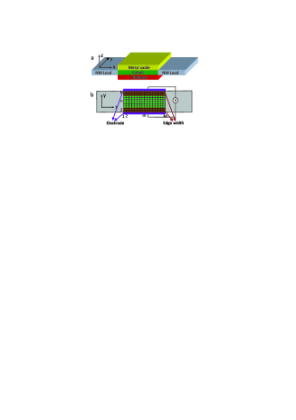
Figure 1: (a) Schematic diagram of the proposed FM moment detector utilizing the ISHE phenomenon. (b) Lattice discretization of the device for tight-binding NEGF calculation (top view). The Hall voltage $V_{t}$ is the potential difference between the two strip electrodes running along the top and bottom edges of the central region. The covered area schematically shows the edge width which will be used for the Hall voltage calculation.

II Model Hamiltonian and Theory

The schematic diagram of the FM moment detector is shown in Fig. 1(a); the central region comprises of a triple-layer structure for the enhancement of RSOC within the FM (Co) layer Miron . Charge accumulation within the Co layer is calculated via tight-binding NEGF method Xing . To perform the tight-binding calculation, the central region of the device is discretized into $(M\times N)$ lattice of points [see Fig. 1(b)]. The conduction electrons within the Co layer experiences the RSOC effect and the $s$-$d$ exchange interaction with the local FM moments $\textbf{M}(\theta,\phi)$. Thus, the Hamiltonian of the central region can be expressed as $H_{C}=H_{K}+H_{M}+H_{Rso}$, where $H_{K}$ is the kinetic term, $H_{M}$ the $s$-$d$ coupling term, and $H_{Rso}$ the RSOC term. The Hamiltonian can be expressed as Rashba :

$$H_{K} = \sum_{mn\sigma}[4td^{\dagger}_{mn\sigma}d_{mn\sigma}$$ (1)

$$- t(d^{\dagger}_{m+1,n\sigma}d_{mn\sigma}+d^{\dagger}_{m,n+1\sigma}d_{mn\sigma}+\mathrm{h.c.})],$$

$$H_{M} = \sum_{mn\sigma}\mathrm{sgn}[\sigma]M\cos(\theta)d^{\dagger}_{mn\sigma}d_{mn\sigma}$$ (2)

$$+M\sin(\theta)e^{i\sigma\phi}d^{\dagger}_{mn\sigma}d_{mn\bar{\sigma}},$$

$$H_{Rso} = \sum_{mn\sigma\sigma^{\prime}}-it_{so}[(d^{\dagger}_{m+1,n}d_{mn}-d^{\dagger}_{m-1,n}d_{mn})\otimes\hat{\sigma}_{y}$$ (3)

$$-(d^{\dagger}_{m,n+1}d_{mn}-d^{\dagger}_{m,n-1}d_{mn})\otimes\hat{\sigma}_{x}],$$

where $M$ denotes the $s$-$d$ coupling strength, $t_{so}=\frac{\alpha}{2a}$ denotes the RSOC strength. Similarly, the Hamiltonian of the normal metal (NM) leads, and the coupling energy between the leads and central region can be expressed as:

$$H_{L(R)} = \sum_{mn\sigma}[4ta^{\dagger}_{mn\sigma}a_{mn\sigma}$$ (4)

$$- t(a^{\dagger}_{m+1,n\sigma}a_{mn\sigma}+a^{\dagger}_{m,n+1\sigma}a_{mn\sigma}+\mathrm{h.c.})].$$

$$H_{T} = \sum_{n\sigma}[t^{\prime}_{L}a^{\dagger}_{0n\sigma}d_{1n\sigma}+t^{\prime}_{R}a^{\dagger}_{M+1,n\sigma}d_{Mn\sigma}+\mathrm{h.c.}].$$ (5)

From the eigenvalue equation of the total Hamiltonian and the definition of retarded Green’s function, one can obtain an equation: $(E-H_{mn}+i\eta)G^{n,n}_{m,m}(\sigma\sigma)=I$. From this relation, one can obtain a series of linear equations involving $G^{n,n}_{m,m}(\sigma\sigma)$ by considering each spatial point $(m,n)$. For instance, within the central region, i.e. $1<m<M$, one obtains:

$$I = [E-4t-\sigma M\cos(\theta)]G^{n,n}_{m,m}(\sigma\sigma)-e^{i\sigma\phi}M\sin(\theta)G^{n,n}_{m,m}(\bar{\sigma}\sigma)+t[G^{n,n}_{m-1,m}(\sigma\sigma)+G^{n,n}_{m+1,m}(\sigma\sigma)$$ (6)

$$+ G^{n-1,n}_{m,m}(\sigma\sigma)+G^{n+1,n}_{m,m}(\sigma\sigma)]+t_{so}[\sigma G^{n,n}_{m+1,m}(\bar{\sigma}\sigma)-iG^{n+1,n}_{m,m}(\bar{\sigma}\sigma)-\sigma G^{n,n}_{m-1,m}(\bar{\sigma}\sigma)+iG^{n-1,n}_{m,m}(\bar{\sigma}\sigma)].$$

Collectively, all these equations can be expressed in matrix form: $(E[I]-[H])[G]^{r}=I$. The infinitely large matrix $[H]$ consists of sub-matrices denoting the Hamiltonian of the central region ($[H_{C}]$) and the coupling coefficients between the two leads and the central region separately ($[\tau_{L/R,C}]$). Following standard procedures in the tight-binding method, one then obtains:

$$(E[I]-[H_{C}]-[\Sigma]^{r}_{L}-[\Sigma]^{r}_{R})[G_{C}]^{r}=I,$$ (7)

in which the non-zero terms of the self energy are: $[\Sigma^{n,n^{\prime}}_{m,m}]^{r}_{L(R)}=[\tau]^{n,n}_{m,0(M+1)}[g^{r}]^{n,n^{\prime}}_{0(M+1),0(M+1)}[\tau]^{n^{\prime},n^{\prime}}_{0(M+1),m}$. The retarded Green’s functions of the isolated left(right) lead $[g^{r}]^{n,n^{\prime}}_{0(M+1),0(M+1)}$ can be expressed as (for the left lead):

$$[g^{r}]^{n,n^{\prime}}_{0,0}=-\frac{1}{t}\sum_{i}\chi_{i}(p_{n})e^{ik_{i}a}\chi_{i}(p_{n^{\prime}}).$$ (8)

In the above, $k_{i}$ is the wave vector along the semi-infinite longitudinal direction, $\chi_{i}(p_{n})$ is the $\tilde{i}$th eigenfunction in the transverse dimension at site $(0,n)$ in the lead, which can be expressed as:

$$\chi_{i}(p_{n})=\sqrt{\frac{2}{N+1}\sin{\frac{i\pi n}{N+1}}}.$$ (9)

The retarded Green’s function of the central region can then be solved by inverting Eq. (7). Thus one can express the lesser Green’s function $[G]^{<}$ via the Langreth formula: $[G]^{<}=[G]^{r}[\Sigma]^{<}[G]^{a}$, in which $[\Sigma]^{<}=\sum_{\mu=L,R}([\Sigma]^{a}_{\mu}-[\Sigma]^{r}_{\mu})f_{\mu}$, with $f_{\mu}$ being the Fermi distribution function within lead $\mu$. The total charge accumulation for a given cell at lattice coordinate $(m,n)$ with an area of $a^{2}$ is given by:

$$\tilde{\rho}_{m,n}=-\frac{ie}{2\pi}\int^{\infty}_{-\infty}Tr[G]^{<}_{mn,mn}(E)dE,$$ (10)

where the trace is over the spin degree of freedom. The surface charge density $\rho_{m,n}$ is then given by $\rho_{m,n}=\frac{\tilde{\rho}_{m,n}}{a^{2}}$.

The Hall voltage at longitudinal position $x=m$ ($V_{tm}$) is given, up to a proportionality constant, by the difference in the surface charge density between the top and bottom edges corresponding to $x=m$, i.e. $V_{tm}\propto\Delta\rho_{m}=\rho_{tm}-\rho_{bm}$. In calculating the charge densities $\rho_{tm}$ and $\rho_{bm}$, we consider a finite width of each edge. The values of $\rho_{tm}$ and $\rho_{bm}$ are averaged over some number of rows ($W$) adjacent to the top and bottom edges, such that $Wa\approx$ 0.3 nm. Thus, the surface charge density difference along $x$-direction is given by:

$$\Delta\rho_{m}=\frac{\sum^{W}_{n=1}\rho_{m,N-n+1}-\rho_{m,n}}{W}.$$ (11)

In practice, the Hall voltage $V_{t}$ is given by the potential difference between the two electrodes. We assume that each electrode runs along the entire length of the edges (i.e., from $m=1$ to $M$). Thus, computationally, the Hall voltage $V_{t}$ is given by the surface charge density difference averaged over the longitudinal dimension, i.e.,

$$\Delta\rho_{av}=\frac{\sum^{M}_{m=1}\sum^{W}_{n=1}\rho_{m,N-n+1}-\rho_{m,n}}{M\times W}.$$ (12)

III Results and Discussion

The following parameters are assumed in the numerical calculations: (i) The device is modeled at room temperature ($T=300$ K); the Fermi energy of the central FM layer is set to $7.38$ eV, which is a typical value for Co Wawrzyniaka . (ii) The lattice cell dimension is set to $a=0.045$ nm, which is significantly smaller than the Fermi wavelength $(a\sim\lambda/10)$, so that the lattice Green’s function model can simulate a continuum system to a good approximation. (iii) The coupling strength is $t=\frac{\hbar^{2}}{2ma^{2}}=18.69$ eV, while for simplicity, the coupling between the lead and the central region is set to $t_{L/R}=0.8t$. (iv) The RSOC strength in Eq. (3) is given by $t_{so}=\frac{\alpha}{2a}$. For a typical FM RSOC material, $\alpha$ lies between $4\times 10^{-11}$ and $3\times 10^{-10}$ eVm Ast ; Henk ; Krupin , which translates to a range of coupling parameter values of $0.4<t_{so}<3.3$ eV. (v) The $s$-$d$ exchange energy is set to $|M|=0.85$ eV Wakoh . (vi) The electrochemical potentials of the two leads are set to $\mu_{L}=-\mu_{R}=2$ eV. (vii) Finally, the central region is discretized into a square lattice of $(M\times N)=(200\times 100)$ of unit cells. This corresponds to an actual dimensions of (9 nm$\times$ 4.5 nm) for the central region.

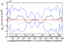
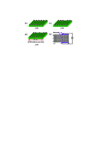
Figure 2: (a) Distribution of $\Delta\rho_{m}$ along the longitudinal $x$-axis. The FM moments in the central region are oriented along the $\pm x$ (blue), $\pm y$ (red) and $\pm z$ (black) directions. The corresponding electron density distributions are schematically depicted in (b), (c) and (d), respectively. Fig (e) shows a possible electrode configuration to detect the Hall voltage when FM moment is along $\pm x$ directions. The following parameter values are assumed: RSOC strength of $t_{so}=3$ eV, bias voltage of $V=4$ eV, and $s$-$d$ coupling strength of $M=0.85$ eV. The central region is discretized into a lattice of $(200\times 100)$ unit cells.

We first calculate the transverse charge density difference of $\Delta\rho_{m}$ as a function of the longitudinal position $x$, when the FM moments in the Co layer are separately oriented along $\pm x$, $\pm y$ and $\pm z$ directions. The results are plotted in Figure 2(a). Our results show that when the FM moments are in the $y$-direction, the spatial charge distribution $\rho_{m,n}$ is symmetric about the central longitudinal axis of $n=(N+1)/2$, resulting in $\Delta\rho_{m}=0$. When the FM moments are switched to $-y$ direction, the charge distribution $\rho_{m,n}$ remains symmetric about the central longitudinal axis, and hence $\Delta\rho_{m}$ is still $0$ [see Fig. 2(b) for a schematic representation]. Thus, when the FM moments of the Co layer are aligned along $\pm y$, no Hall voltage would be observed. By contrast, when the FM moments are oriented along the $x$-direction, $\Delta\rho_{m}$ is symmetric about the central point $(m,n)=((M+1)/2,(N+1)/2)$ [see Figs. 2(a) and (c)]. Furthermore, the sign of $\Delta\rho_{m}$ is reversed when the FM moments are switched to the $-x$ direction. However, when averaged along the entire edge, the surface charge density difference will be $\Delta\rho_{av}=0$ due to the point symmetry. However, if the Hall electrodes extend to only half the entire length of the top and bottom edges [as shown schematically in Fig. 2(e)], a finite Hall voltage can still be detected.

Of greater interest is the case where the FM moments are along the out-of-plane $z$-direction. The charge density difference $\Delta\rho_{m}$ is symmetric about the central vertical axis, i.e. $m=(M+1)/2$. Thus, a finite $\Delta\rho_{av}$, i.e., a Hall voltage $V_{t}$ is generated [see Figs. 2(a) and (d)]. Since only charge current but not spin current is injected into the system, the above can be regarded as a charge current-induced ISHE in FM metal with RSOC.

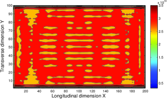
Figure 3: The spatial distribution of $\rho_{m,n}$ (in unit of $\frac{e}{m^{2}}$). The longitudinal and transverse dimensions are expressed in unit of the lattice constant $a$. The $s$-$d$ coupling strength is $M=0.85$ eV, the RSOC strength is $t_{so}=3$ eV, the bias voltage is $V=4$ eV, the central region is a $(200\times 100)$ lattice ($9$ nm $\times 4.5$ nm).

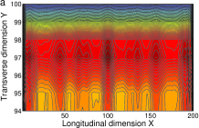
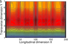
Figure 4: The detailed distribution of $\rho_{tm}$ and $\rho_{bm}$ (in unit of $\frac{e}{m^{2}}$) at (a) the top, and (b) bottom edges of Fig. 3. The longitudinal and transverse dimensions are expressed in unit of the lattice constant $a$.

In the following, we will investigate this charge current-driven ISHE in greater detail. The spatial distribution of $\rho_{m,n}$ is plotted over the central region when the FM moments are in the $+z$-direction [see Fig. 3]. For clarity, the detailed distribution of charge densities $\rho_{tm}$ and $\rho_{bm}$ are shown in Figs. 4(a) and (b). It is observed that the surface charge density is larger along the top edge, which will result in a finite Hall voltage or ISHE effect.

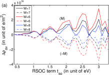
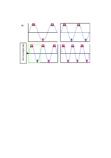
Figure 5: (a) The oscillatory increase of $\Delta\rho_{av}$ with the RSOC strength $t_{so}$, for different edge width $W$ and FM moment orientations (solid lines for $z$, dashed lines for $-z$ ). The central region is discretized into a $(200\times 100)$ lattice, with dimensions (9 nm$\times$4.5 nm). The $s$-$d$ coupling strength is $M=0.85$ eV, while the bias voltage is $V=4$ V. (b) The schematic diagram of the spin electron distribution due to Yang-Mills-like Lorentz force. The number of Hall deflection pairs increases with increasing RSOC strength.

Fig. 5(a) shows the dependence of $\Delta\rho_{av}$ on the RSOC strength $t_{so}$ for different edge width $W$. $\Delta\rho_{av}$, and hence the Hall voltage $V_{t}$ across the central region, show an increasing trend with the RSOC strength $t_{so}$, but in an oscillatory manner. The physics underlying this oscillatory increase can be understood in terms of the Yang-Mills-like Lorentz force arising from the RSOC gauge Tan ; Shen . Here, the FM moments $M$ merely play the role of sustaining a vertical spin polarization of current but do not contribute directly to the Lorentz force. The Lorentz force leads to the transverse separation of electrons of opposite spins [shown schematically in Fig. 5(b)], which we term as “Hall deflection pair”. Since there are unequal number of charges on the two transverse sides, each Hall deflection pair will contribute to a charge Hall voltage. For a fixed $M$, an increase in the RSOC strength results in an increasing number of Hall deflection pairs along the length of the device, as shown in Fig. 5(b). The charge imbalance in a Hall deflection pair coupled with the increase in the number of such pairs with the RSOC strength provide a heuristic explanation of the oscillatory increase of $\Delta\rho_{av}$ and the Hall voltage with the RSOC strength. The sign of $\Delta\rho_{av}$ can be reversed by switching the orientation of FM moment between $\pm z$. Furthermore, $\Delta\rho_{av}$ is not sensitive to the definition of edge, i.e. the general trend remains unchanged for the range of edge width $W$ considered in our calculation.

Previous work on RSOC in semiconductors has shown that when the surface charge density difference is in the order of $10^{12}e/\mathrm{m}^{2}$, the generated Hall voltage will be large enough for detection (0.1 mV) Li . The electron density in our metallic FM RSOC device will be much higher than that in semiconductors, so that $\Delta\rho_{av}$ could attain a value of the order of $10^{16}e/\mathrm{m}^{2}$ and generate a sizable Hall voltage of $V_{t}\approx 1V$. By selecting optimal $t_{so}$ which corresponds to the peak Hall voltage values (see Fig. 5), we conjecture that a reasonably large $\Delta\rho_{av}$, hence $V_{t}$ can be measured when the FM moments are oriented along the out-of-plane $z$ axis. The charge density difference $\Delta\rho_{av}$ switches in sign upon reversal of the FM moments to the $-z$ direction. The resulting large difference in the Hall voltage corresponding to the two FM orientations ($\pm z$) suggests that the ISHE can be utilized in a metal FM RSOC system for the sensitive detection of the FM moment orientation.

In summary,we have investigated the inverse spin Hall effect (ISHE) which is induced by the combination of RSOC and $s$-$d$ coupling to the FM moments. A Hall voltage is generated when the FM moments are oriented in the perpendicular-to-plane direction. The Hall voltage increases in an oscillating manner with the RSOC strength $t_{so}$. The polarity of the Hall voltage is reversed when the FM moment is switched to the opposite direction. This property suggests the utility of the ISHE in FM metals with strong RSOC effect for the detection of the FM moment direction, e.g., as a possible memory readback mechanism.

- (1) P. Gambardella, S. Rusponi, M. Veronese, S. S. Dhesi, C. Grazioli, A. Dallmeyer, I. Cabria, R. Zeller, P. H. Dederichs, K. Kern, C. Carbone, and H. Brune, Science 300, 1130 (2003).
- (2) C. R. Ast, J. Henk, A. Ernst, L. Moreschini, M. C. Falub, D. Pacilé, P. Bruno, K. Kern, and M. Grioni, Phys. Rev. Lett. 98, 186807 (2007).
- (3) S. LaShell, B. A. McDougall, and E. Jensen, Phys. Rev. Lett. 77, 3419 (1996).
- (4) I. M. Miron, G. Gaudin, S. Auffret, B. Rodmacq, A. Schuhl, S. Pizzini, J. Vogel, and P. Gambardella, Nature Materials 9, 230 (2010).
- (5) E. Saitoh, M. Ueda, H. Miyajima, and G. Tatara, Applied Physics Letters 88, 182509 (2006).
- (6) E. M. Hankiewicz, J. Li, T. Jungwirth, Q. Niu, S.-Q. Shen, and J. Sinova, Phys. Rev. B 72, 155305 (2005).
- (7) S. O. Valenzuela and M. Tinkham, Nature 442, 176 (2006).
- (8) J. J. Zhang, F. Liang, and J. Wang, Eur. Phys. J. B 72, 105 (2009).
- (9) E. Saitoh, M. Ueda, H. Miyajima, and G. Tatara, Appl. Phys. Lett. 88, 182509 (2006).
- (10) T. Kimura, Y. Otani, T. Sato, S. Takahashi, and S. Maekawa, Phys. Rev. Lett. 98, 156601 (2007).
- (11) Y. Xing, Q.-F. Sun, and J. Wang, Phys. Rev. B 75, 075324 (2007).
- (12) J. Li and S. Q. Shen, Phys. Rev. B 76, 153302 (2007).
- (13) K. Ando and E. Saitoh, J. Appl. Phys. 108, 113925 (2010).
- (14) E. I. Rashba, Phys. Rev. B 70, 161201(R) (2004).
- (15) M. Wawrzyniaka, M. Mackowski, Z. Sniadecki, B. Idzikowski, and J. Martinek, Acta Physica Polonica A. 118, 375 (2010).
- (16) J. Henk, M. Hoesch, J. Osterwalder, A. Ernst1, and P. Bruno, J. Phys.: Condens. Matter 16, 7581 (2004).
- (17) O. Krupin, G. Bihlmayer, K. Starke, S. Gorovikov, J. E. Prieto, K. Döbrich, S. Blügel, and G. Kaindl, Phys. Rev. B 71 (2005).
- (18) S. Wakoh and J. Yamashita, Journal of the Physical Society of Japan 28, 1151 (1970).
- (19) S. G. Tan, M. B. A. Jalil, X.-J. Liu, and T. Fujita, Phys. Rev. B. 78, 245321 (2008).
- (20) S.-Q. Shen, Phys. Rev. Lett. 95, 187203 (2005).