A catalog of 132,684 clusters of galaxies identified from Sloan Digital Sky Survey III

Abstract

Using the photometric redshifts of galaxies from the Sloan Digital Sky Survey III (SDSS-III), we identify 132,684 clusters in the redshift range of $0.05\leq z<0.8$. Monte Carlo simulations show that the false detection rate is less than 6% for the whole sample. The completeness is more than 95% for clusters with a mass of $M_{200}>1.0\times 10^{14}~{}M_{\odot}$ in the redshift range of $0.05\leq z<0.42$, while clusters of $z>0.42$ are less complete and have a biased smaller richness than the real one due to incompleteness of member galaxies. We compare our sample with other cluster samples, and find that more than 90% of previously known rich clusters of $0.05\leq z<0.42$ are matched with clusters in our sample. Richer clusters tend to have more luminous brightest cluster galaxies (BCGs). Correlating with X-ray and the Planck data, we show that the cluster richness is closely related to the X-ray luminosity, temperature, and Sunyaev–Zel’dovich measurements. Comparison of the BCGs with the SDSS luminous red galaxy (LRG) sample shows that 25% of LRGs are BCGs of our clusters and 36% of LRGs are cluster member galaxies. In our cluster sample, 63% of BCGs of $r_{\rm petro}<19.5$ satisfy the SDSS LRG selection criteria.

1. Introduction

Clusters of galaxies are usually located at the knots of the filamentary structures in the universe. They are the most massive bound systems to trace the large-scale structure (Bahcall, 1988; Postman et al., 1992; Carlberg et al., 1996; Bahcall et al., 1997). Statistical studies of clusters provide very powerful constraint on the cosmological parameters (see a review in Allen et al., 2011) by using, e.g., cluster mass function (Reiprich & Böhringer, 2002; Seljak, 2002; Dahle, 2006; Pedersen & Dahle, 2007; Rines et al., 2007; Wen et al., 2010) and gas fraction in massive clusters (Allen et al., 2008). Clusters are also important laboratories to investigate the evolution of galaxies in dense environment (Dressler, 1980; Butcher & Oemler, 1978, 1984; Goto et al., 2003) and act as natural telescope to study lensed high-redshift faint background galaxies (Blain et al., 1999; Smail et al., 2002; Metcalfe et al., 2003; Santos et al., 2004). As a large number of clusters have been detected (Koester et al., 2007a; Wen et al., 2009), the distributions of galaxy clusters are used to detect the baryon acoustic oscillation of the universe (Estrada et al., 2009; Hütsi, 2010; Hong et al., 2012). Correlation of background objects with a large sample of clusters shows the effects of weak lensing and spectra line absorption (Myers et al., 2005; Lopez et al., 2008).

Galaxy clusters have been found from single-band optical imaging data (e.g., Abell, 1958; Postman et al., 1996), multicolor photometric data (e.g., Gladders & Yee, 2005; Koester et al., 2007a) and spectroscopic redshift surveys (e.g., Huchra & Geller, 1982; Yang et al., 2005). In addition, clusters have also been found from X-ray surveys (e.g., Böhringer et al., 2000, 2004). At millimeter wavelength, the Sunyaev–Zel’dovich (SZ) effect has recently used to find clusters, which is insensitive to cluster redshift (Carlstrom et al., 2000). Hundreds of SZ clusters have been identified (Marriage et al., 2011; Planck Collaboration et al., 2011).

The Sloan Digital Sky Survey (SDSS; York et al., 2000) offers an opportunity to produce the largest and most complete cluster sample. It provides photometry in five broad bands ($u$, $g$, $r$, $i$, and $z$) covering 14,000 deg² and the follow-up spectroscopic observations. The photometric data reach a limit of $r=22.2$ (Stoughton et al., 2002) with the star–galaxy separation reliable to a limit of $r=21.5$ (Lupton et al., 2001). The spectroscopic survey observes galaxies with an extinction-corrected Petrosian magnitude of $r<17.77$ for the main galaxy sample (Strauss et al., 2002) and $r<19.5$ for the luminous red galaxy (LRG) sample (Eisenstein et al., 2001). Galaxy clusters or groups have been found by using the SDSS spectroscopic data (e.g., Merchán & Zandivarez, 2005; Berlind et al., 2006) and the photometric data (e.g., Goto et al., 2002; Koester et al., 2007a; Wen et al., 2009; Hao et al., 2010; Szabo et al., 2011).

For large samples of galaxy clusters, the determination of optical richness still has a large uncertainty because of difficulties in the discrimination of cluster member galaxies from background galaxies using photometric data. This causes a large scatter when the optical richness is used to represent the cluster mass for the constraint of cosmological parameters (Rykoff et al., 2008; Rozo et al., 2009b; Wen et al., 2010).

In this paper, we improve the method of Wen et al. (2009) using photometric redshifts to identify a large sample of galaxy clusters up to $z\sim 0.8$. In Section 2, we identify clusters using a new cluster detection algorithm and determine a cluster richness that is closely related to cluster mass. In Section 3, we compare our sample with the previous cluster samples from the SDSS, and correlate the cluster richness with X-ray and SZ measurements. In Section 4, we study the brightest cluster galaxies (BCGs) and cross-identify them with the SDSS LRGs. A summary is presented in Section 5.

Throughout this paper, we assume a $\Lambda$CDM cosmology, taking $H_{0}=$100 $h$ ${\rm km~{}s}^{-1}$ ${\rm Mpc}^{-1}$, with $h=0.72$, $\Omega_{m}=0.3$ and $\Omega_{\Lambda}=0.7$.

2. Clusters identified from SDSS-III

Wen et al. (2009) identified 39,668 galaxy clusters from the SDSS DR6 by the discrimination of member galaxies of clusters using photometric redshifts (hereafter photo-$z$s) of galaxies. Wen & Han (2011) improved the method and successfully identified the high-redshift clusters from the deep fields of the Canada–France–Hawaii Telescope Wide (CFHT) survey, the CHFT Deep survey, the Cosmic Evolution Survey, and the Spitzer Wide-area InfraRed Extragalactic survey. Here, we follow and improve the algorithm to identify clusters from SDSS-III (SDSS Data Release 8; Aihara et al., 2011). We first use the SDSS data to determine scaling relations for cluster mass and radius which will be used in the cluster detection.

2.1. SDSS Data

The galaxy data of 14,000 deg² are downloaded from the SDSS-III database. The photo-$z$s, the $K$-corrections, and the absolute magnitudes are obtained from the table Photoz in which photo-$z$s are estimated based on the method of Csabai et al. (2007). We remove objects with deblending problems and saturated objects using the flags.

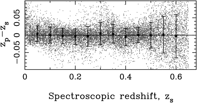
Figure 1.— Difference between spectroscopic redshift $z_{\rm s}$ and photometric redshift $z_{\rm p}$ for galaxies of the SDSS-III.

As shown in Figure 1, the uncertainties of photo-$z$s are $\sim$0.025–0.030 in the redshift range $z<0.45$. They become larger at higher redshifts. In the following analysis, we assume that the uncertainty of photo-$z$, $\sigma_{z}$, increases with redshift in the form of $\sigma_{z}=\sigma_{0}(1+z)$ for all galaxies. Here, we discard those galaxies with a large photo-$z$ error $z{\rm Err}>0.08(1+z)$, i.e., about $3\,\sigma_{z}$, which suffer bad photometry or contamination of stars. This procedure removes 20% of objects, most of which are faint objects ($r>21$) with large photometric errors.

BCGs are the most luminous members of clusters. Generally, the BCGs are elliptical galaxies and have smaller photo-$z$ error than other member galaxies. Proper selection of BCGs can be helpful to identify clusters and estimate the cluster parameters. To get right BCGs, we select those galaxies as BCG candidates which have a photo-$z$ error $z{\rm Err}\leq 0.055(1+z)$ and a galaxy ellipticity in the $r$ band less than 0.7.

2.2. Scaling relations for cluster mass and radius

Figure 2.— Upper: scaling relation between cluster radius $r_{200}$ and total luminosity within a radius of 1 Mpc in units of $L^{\ast}$. Lower: scaling relation between cluster mass $M_{200}$ and richness $R_{L\ast}$. The solid lines show the best-fit relations. Data are derived for clusters compiled by Wen et al. (2010).

The cluster mass and radius are two fundamental parameters for clusters. The widely used are $r_{200}$, the radius within which the mean density of a cluster is 200 times of the critical density of the universe, and $M_{200}$, the cluster mass within $r_{200}$.

We use the SDSS data of known clusters to get the scaling relations for $r_{200}$ and $M_{200}$. Here, we take the clusters whose masses or radii have been estimated by X-ray or weak-lensing methods as compiled by Wen et al. (2010). For each cluster, we calculate the total luminosities of cluster member candidates in the SDSS $r$-band within a radius of 1 Mpc from its BCG by summing luminosities of member galaxy candidates brighter than $M^{e}_{r}(z)\leq-20.5$ but fainter than the BCG within a photo-$z$ gap of $z\pm 0.04(1+z)$, with a local background subtraction. Here, $M^{e}_{r}$ is the evolution-corrected absolute magnitude in the $r$ band, $M^{e}_{r}(z)=M_{r}(z)+Qz$, where we adopt a passive evolution of $Q=1.62$ (Blanton et al., 2003). To estimate local background, we follow the method analogous to Popesso et al. (2004). For each cluster, we divide the annuals between 2 and 4 Mpc from its BCG into 48 sections with equal area. Within the same magnitude and photo-$z$ range, we calculate the total luminosity in each sector and estimate the mean value and its root mean square. The regions with luminosities larger than 3$\,\sigma$ are discarded and the mean is recalculated to be the local background. We measure the total luminosity of cluster member candidates in units of $L^{\ast}$, here $L^{\ast}$ is the evolved characteristic luminosity of galaxies in the $r$ band, defined as $L^{\ast}(z)=L^{\ast}(z=0)10^{0.4Qz}$ (Blanton et al., 2003).

In Figure 2, we show the correlation between cluster radius $r_{200}$ and total luminosity within a radius of 1 Mpc, $L_{\rm 1Mpc}$. The best fit gives

$$\log r_{200}=(-0.57\pm 0.09)+(0.44\pm 0.05)\log L_{\rm 1Mpc},$$ (1)

where $r_{200}$ is in units of Mpc and $L_{\rm 1Mpc}$ is in units of $L^{\ast}$. Similarly, we also get the total $r$-band luminosity within the radius of $r_{200}$, $L_{200}$, in units of $L^{\ast}$, with a background subtraction. In this paper, we define the cluster richness as $R_{L\ast}=L_{200}/L^{\ast}$. We find that cluster mass $M_{200}$ and cluster richness are closely correlated as (lower panel of Figure 2)

$$\log M_{200}=(-1.49\pm 0.05)+(1.17\pm 0.03)\log R_{L\ast},$$ (2)

where $M_{200}$ is in units of $10^{14}~{}M_{\odot}$. Using these scaling relations, we can estimate the cluster radius and mass from observables of $L_{\rm 1Mpc}$ and $L_{200}$ or $R_{L\ast}$. We have shown in our previous work that the measurements of the total luminosity or richness are robust for adopting different widths of the photo-$z$ gap (Wen et al., 2009). In the following, we extrapolate these relations to lower richness for cluster identification. Based on the estimated richness, we identify clusters with a richness threshold of $R_{L\ast}\geq 12$.

2.3. Cluster detection algorithm

Table 1Clusters of Galaxies Identified from the SDSS-III

Name	R.A.BCG	Decl.BCG	$z_{\rm p}$	$z_{\rm s,BCG}$	$r_{\rm BCG}$	$r_{200}$	$R_{L\ast}$	$N_{200}$	Other Catalogs
	(deg)	(deg)				(Mpc)
(1)	(2)	(3)	(4)	(5)	(6)	(7)	(8)	(9)	(10)
WHL J000000.6$+$321233	0.00236	32.20925	0.1274	$-1.0000$	14.92	1.72	70.63	24	Abell
WHL J000002.3$+$051718	0.00957	5.28827	0.1696	$-1.0000$	16.20	0.94	17.48	9
WHL J000003.3$+$311354	0.01377	31.23175	0.5428	$-1.0000$	20.17	0.87	14.27	8
WHL J000003.5$+$314708	0.01475	31.78564	0.0932	$-1.0000$	15.18	0.94	16.97	9
WHL J000004.7$+$022826	0.01945	2.47386	0.4179	$-1.0000$	19.32	0.95	13.71	10
WHL J000004.9$-$033248	0.02024	$-3.54679$	0.5968	$-1.0000$	20.67	1.00	19.19	11
WHL J000005.5$+$354610	0.02303	35.76957	0.4762	$-1.0000$	19.59	0.91	15.58	9
WHL J000006.0$+$152548	0.02482	15.42990	0.1656	$-1.0000$	16.60	1.13	23.53	19	maxBCG,WHL09,GMBCG
WHL J000006.3$+$221220	0.02643	22.20558	0.3985	$-1.0000$	19.36	0.84	12.73	11
WHL J000006.6$+$100648	0.02755	10.11333	0.3676	$-1.0000$	19.07	0.93	16.73	13
WHL J000006.6$+$315235	0.02762	31.87626	0.2134	$-1.0000$	17.11	1.18	28.58	15
WHL J000006.6$+$292129	0.02765	29.35813	0.2489	$-1.0000$	18.13	0.92	15.11	16
WHL J000007.1$-$092910	0.02957	$-9.48607$	0.3332	$-1.0000$	19.11	0.80	12.81	13	AMF
WHL J000007.6$+$155003	0.03177	15.83424	0.1436	0.1528	15.99	1.17	34.11	27	Abell,maxBCG,WHL09,GMBCG,AMF
WHL J000007.7$+$185245	0.03208	18.87909	0.4347	$-1.0000$	18.95	1.03	20.47	12

Note. — Column 1: Cluster name with J2000 coordinates of cluster; Column 2: R.A. (J2000) of cluster and BCG; Column 3: Decl. (J2000) of cluster and BCG; Column 4: photometric redshift of cluster; Column 5: spectroscopic redshift of BCG, $-1.0000$ means not available; Column 6: $r$-band magnitude of BCG; Column 7: $r_{200}$ of cluster (Mpc); Column 8: cluster richness; Column 9: number of member galaxy candidates within $r_{200}$; Column 10: other catalogs containing the cluster: Abell (Abell, 1958; Abell et al., 1989); maxBCG (Koester et al., 2007a); WHL09 (Wen et al., 2009); GMBCG (Hao et al., 2010); AMF (Szabo et al., 2011).

(This table is available in its entirety in a machine-readable form in the online journal. A portion is shown here for guidance regarding its form and content.)

In Wen et al. (2009), we identified a cluster if more than eight member galaxies of $M_{r}\leq-21$ (without evolution correction and different from $M^{e}_{r}(z)$ in this paper) are found within a radius of 0.5 Mpc and a photo-$z$ gap of $z\pm 0.04(1+z)$. The richness was estimated to be the number of galaxies within a radius of 1 Mpc which may be systematically smaller than the true radius for rich clusters but larger than that for poor clusters. Note also that the radius of 0.5 Mpc for cluster identification is not the same as the radius of 1 Mpc for richness estimate.

With the tight scaling relations shown in Section 2.2, we can improve the method of Wen et al. (2009) and Wen & Han (2011) to identify clusters from the SDSS-III. Our new algorithm includes following steps.

1. For each galaxy at a given photometric redshift, $z$, we count the number of luminous member galaxies of $M^{e}_{r}(z)\leq-20.5$ within a radius of 0.5 Mpc and a photo-$z$ gap of $z\pm 0.04(1+z)$, $N_{\rm 0.5Mpc}$.

2. To get cluster candidates, we apply the friend-of-friend algorithm (Huchra & Geller, 1982) to the luminous galaxies using a linking length of 0.5 Mpc in the transverse direction and a photo-$z$ difference of $0.06(1+z)$. The linked galaxy with the maximum $N_{\rm 0.5Mpc}$ is taken as the temporary center of a cluster candidate. If two or more galaxies have the same maximum number, the brightest one is taken as the temporary central cluster galaxy. Then, we obtain a temporary list of cluster candidates.

3. For each cluster candidate at $z$, we assume that the galaxies of $M^{e}_{r}(z)\leq-20.5$ within a radius of 1 Mpc from the temporary central galaxy and the photo-$z$ gap of $z\pm 0.04(1+z)$ are member galaxies. The cluster redshift $z_{\rm p}$ is then defined to be the median value of the photometric redshifts of the recognized “members”.

4. We recognize the BCG of a cluster candidate as the brightest galaxy from the BCG candidate sample within a radius of 0.5 Mpc from the temporary center and the photo-$z$ gap of $z\pm 0.04(1+z)$. As a new development in this paper, we use the BCG as the center of a cluster and calculate $L_{\rm 1Mpc}$ from the estimated redshift. Subsequently, we get $r_{200}$ using Equation (1) and measure $R_{L\ast}$ from $L_{200}$ within the estimated $r_{200}$ for each cluster candidate. Note that the local background has been subtracted already here.

5. We define a galaxy cluster if $R_{L\ast}\geq 12$, which corresponds to $M_{200}\sim 0.6\times 10^{14}~{}M_{\odot}$ using Equation (2). Note that a cluster candidate at low richness may be contaminated by a small number of bright field galaxies with their photo-$z$s seriously overestimated. To avoid such contamination, we require the number of galaxies within a radius of $r_{200}$ and a photo-$z$ gap of $z\pm 0.04(1+z)$, $N_{200}\geq 8$. This assures that the cluster sample above the detection criteria has a high completeness and a low false detection rate (see Sections 2.5 and 2.6). After we get the cluster candidate list, we merge possible repeatedly identified clusters which may survive in the previous procedure by using the friend-of-friend algorithm. If two cluster candidates have photo-$z$ difference less than $0.06(1+z)$ and a projection separation less than $r_{200}$, we merge the cluster candidates as one cluster, and the poorer one is then removed from the list.

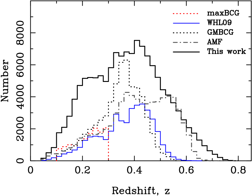
Figure 3.— Redshift distribution of the 132,684 identified clusters in the SDSS-III together with those of 13,823 maxBCG clusters within $0.1\leq z\leq 0.3$ (Koester et al., 2007a), 39,668 WHL09 clusters within $0.05<z<0.6$ (Wen et al., 2009), 55,424 Gaussian Mixture Brightest Cluster Galaxy (GMBCG) clusters within $0.1<z<0.55$ (Hao et al., 2010) and 69,173 adaptive matched-filter (AMF) clusters within $0.045\leq z<0.78$ (Szabo et al., 2011).
(A color version of this figure is available in the online journal.)

Finally, we visually inspect the color images on the SDSS Web site for all cluster candidates. About 5000 (3.6%) cluster candidates are obvious contaminations from bad photometries and are removed. By this procedure, we discovered 68 lensing systems from the color images (Wen et al., 2011).

After above procedures, we find 132,684 clusters in the redshift of $0.05\leq z<0.8$ from the SDSS-III data. All clusters are listed in Table 1. Figure 3 show the redshift distribution of the identified clusters in the SDSS-III which is compared with those of the maxBCG (Koester et al., 2007a), WHL09 (Wen et al., 2009), Gaussian Mixture Brightest Cluster Galaxy (GMBCG; Hao et al., 2010) and adaptive matched-filter (AMF; Szabo et al., 2011) samples. Our new sample has a peak at $z\sim 0.42$ and the number of our clusters is nearly two times as the previously largest AMF sample by Szabo et al. (2011). The clusters of $z<0.42$ seem to be a complete sample. Because of the magnitude limit of the SDSS photometric data, the member galaxies of $z>0.42$ are incomplete for the threshold of $M^{e}_{r}(z)=-20.5$, so that clusters of $z>0.42$ have a biased smaller richness than the real one because of missing members. In the following, we only consider clusters of $z<0.42$ when we compare our richness with other richness estimates and X-ray measurements.

2.4. Redshift uncertainty

Figure 4.— Distribution of the difference between photometric and spectroscopic redshifts in the four redshift ranges. The solid line is the best fit with a Gaussian function. The parameters, i.e., the offset $\delta$ and the standard deviation $\sigma$, of the Gaussian function are marked on the left of each panel.

Using the SDSS spectroscopic data, we can get the spectroscopic redshift of identified clusters and verify the accuracy of their photometric redshifts. The spectroscopic redshift of a cluster is taken to be that of its BCG. We find that the BCGs of 38,116 clusters have spectroscopic redshifts.

Figure 4 shows the distribution of the difference between photometric and spectroscopic redshifts, $z_{\rm p}-z_{\rm s,BCG}$. The standard deviations roughly indicate the accuracy of redshift estimate for clusters. In each panel, we fit the distribution of $z_{\rm p}-z_{\rm s,BCG}$ with a Gaussian function. The systematic offset $|\delta|$ of the fitting is less than $0.004$, and the standard deviation $\sigma$ is less than 0.018.

2.5. Completeness of cluster detection

Figure 5.— Correlation between input richness and output richness for the mock clusters. The solid line shows the best-fit relation.

Figure 6.— Detection rate of the mock clusters as a function of redshift (the upper panel) and cluster mass, $M_{200}$ (the lower panel).

We use Monte Carlo simulation to test the completeness of our sample. Mock clusters are simulated with assumptions for their distributions and then added to the real data of the SDSS. The cluster detection algorithm is applied to the combined data to find the input mock clusters. The detection rate of mock clusters is considered as the indication of completeness of our detection procedure.

First, we generate a population of halos with masses $M_{200}\geq 0.6\times 10^{14}~{}M_{\odot}$ following a mass function of Jenkins et al. (2001) in a cosmology with $\Omega_{m}=0.3$ and $\sigma_{8}=0.9$ in the redshift range of $0.05<z<0.60$. Then, we relate the cluster mass to cluster richness (i.e., total luminosity in units of $L^{\ast}$) by

$$\log M_{200}=-1.49+1.17\log(C\times R_{L\ast,\rm in}),$$ (3)

where $C$ is a scaling factor between input richness $R_{L\ast,\rm in}$ and output richness $R_{L\ast,\rm out}$ of our detection procedure. The discrepancy between $R_{L\ast,\rm in}$ and $R_{L\ast,\rm out}$ is caused by the uncertainty of galaxy photo-$z$. Because the Equation (2) is obtained for the estimated richness based on the SDSS data, we adjust this factor $C$ to make output richness consistent with Equation (2). We first set $C=1$ for Equation (3) to get input richness. Member galaxies are simulated for each halo within a radius of $r_{200}$. The luminosity function and density profile of member galaxies are taken as described in Wen et al. (2009). Here, the luminosities of member galaxies are evolution-corrected, as mentioned in Section 2.2. We assume that the uncertainty of photometric redshift of member galaxies follows a Gaussian probability function with a standard deviation of $\sigma_{z}$, but varies with redshift in the form of $\sigma_{z}=0.03(1+z)$.

We add the mock clusters into the real SDSS data and apply our cluster detection algorithm to measure the output richness. Figure 5 shows the correlation between the input richness and the output richness. The best fit gives

$$R_{L\ast,\rm out}=(-0.52\pm 0.16)+(0.81\pm 0.01)R_{L\ast,\rm in}.$$ (4)

Therefore, we get the factor $C=1/0.81$ for Equation (3) so that the output richness $R_{L\ast,\rm out}$ can be related to cluster mass by Equation (2).

Subsequently, we use Equation (3) to get a new population of input richness. Again, we apply our method to detect the mock clusters. A cluster is detected if the output richness $R_{L\ast,\rm out}\geq 12$ and $N_{200}\geq 8$. The detection rate is given to be the number of detected mock clusters divided by the total number of added mock clusters. Figure 6 shows the detection rate as a function of redshift. The detection rate is nearly 100% for clusters with masses $M_{200}>2\times 10^{14}~{}M_{\odot}$ (richness $R_{L\ast,\rm out}>34$) up to redshift of $z\sim 0.5$, and $\sim$75% for clusters of $M_{200}>0.6\times 10^{14}~{}M_{\odot}$ (richness $R_{L\ast,\rm out}>12$) up to redshift of $z\sim 0.42$. The detection rate drops at higher redshifts, because the member galaxy selection of our algorithm is consistent up to $z\sim 0.42$, as mentioned in Section 2.3. In Figure 6, we also show the detection rate as a function of cluster mass for clusters of $z<0.42$. More than 95% of clusters of $M_{200}>1\times 10^{14}~{}M_{\odot}$ are detected.

2.6. False detection rate

Figure 7.— False detection rate as a function of cluster richness.

The presence of the large-scale structures makes it possible to detect false clusters because of projection effect. We perform a Monte Carlo simulation with the real SDSS data to estimate the false detection rate. First, we discard the member candidates of identified clusters within a radius of $r_{200}$ and a photo-$z$ gap of $z\pm 0.04(1+z)$. Second, we shuffle the data following Wen & Han (2011). Our new cluster detection algorithm is applied to the shuffled data. After above procedures, we get the “false clusters” which satisfy the criteria of $R_{L\ast}\geq 12$ and $N_{200}\geq 8$. The false detection rate is calculated to be the total number of “false clusters” identified from the shuffled data divided by the number of clusters identified from the original SDSS data. We show that the false detection rate is 6.0% for a cluster richness of 12, but decreases to less than 1% for a richness of 23 (see Figure 7).

Note that we have removed some obvious contaminations from cluster list in the cluster identification (Section 2.3). Here, most of the contaminations cannot be found when shuffling the cataloged galaxy data. Hence, removing the contaminations slightly decreases the false detection rate.

3. Comparison with previous cluster samples

We compare our cluster sample in this paper (hereafter WHL12) with previous ones, including the classical Abell sample from the Palomar Sky Survey (Abell et al., 1989), the maxBCG (Koester et al., 2007a), WHL09 (Wen et al., 2009), GMBCG (Hao et al., 2010) and AMF (Szabo et al., 2011) cluster samples from the SDSS. We also compare our clusters with X-ray and SZ cluster samples.

3.1. Comparison with the Abell clusters

We get the Abell cluster sample (Abell et al., 1989) from the NASA/IPAC Extragalactic Database. For the Abell clusters without redshift measurements, we take their redshifts from the SDSS photo-$z$ data. There are 1844 Abell clusters with redshifts $z>0.05$ in the sky coverage of SDSS-III, of which 1688 (92%) clusters are within a projected separation of $r_{200}$ and redshift difference of $|\Delta z|\leq 0.05$ (about 2 $\sigma$ of the uncertainty of the redshift difference) from the WHL12 clusters. The non-matched Abell clusters are relatively poor clusters or projected to neighbors of the large scale structure (Wen et al., 2009). We mark the Abell clusters in Column 10 of Table 1.

3.2. Comparison with the maxBCG clusters

Figure 8.— Distribution of redshift differences between the WHL12 clusters and the maxBCG, WHL09, GMBCG, and AMF clusters within a projected separation of $r_{200}$.

Figure 9.— Upper: matching rate between the WHL12 clusters and the maxBCG clusters, in the same sky coverage of the SDSS DR4, as a function of redshift. Lower: matching rate between the clusters of $0.1<z<0.3$ in the two samples as a function of cluster richness. The left panels show the matching rate of the WHL12 clusters to the maxBCG clusters, and the right ones are the matching rate of the maxBCG clusters to the WHL12 clusters.

Koester et al. (2007a, b) developed a “red-sequence cluster finder”, maxBCG, to detect clusters dominated by red galaxies. They identify clusters with a richness of $N_{\rm gal}\geq 10$, where $N_{\rm gal}$ is the number of galaxies brighter than $0.4L^{\ast}$ in the $i$ band within $r_{200}$ and $2\,\sigma$ of the ridgeline colors. From the sky coverage of the SDSS DR4, they obtained a complete volume-limited sample containing 13,823 clusters in the redshift range of $0.1\leq z\leq 0.3$. The maxBCG sample is approximately 85% complete for the clusters with masses $M>1\times 10^{14}~{}M_{\odot}$.

We cross-match the WHL12 clusters with the maxBCG clusters in the sky coverage of the SDSS DR4. Figure 8 shows the redshift difference ($\Delta z=z_{\rm p}-z_{\rm maxBCG}$) between the WHL12 clusters and the maxBCG clusters (also the WHL09, GMBCG, and AMF clusters for discussion below) within a projected separation of $r_{200}$. It shows that a value of $|\Delta z|\leq 0.05$ is an appropriate selection threshold for cluster matching in redshift difference (top left panel of Figure 8). We find that 10,301 (75%) of 13,823 maxBCG clusters are matched with the WHL12 clusters within a separation of $r_{200}$ and a redshift difference of $|\Delta z|\leq 0.05$. Figure 9 shows the matching rates between the WHL12 clusters and the maxBCG clusters as a function of redshift. We find that 70%–80% maxBCG clusters are matched with the WHL12 clusters in the redshift range of $0.1\leq z\leq 0.3$, while only 30%–40% of the WHL12 clusters are matched with the maxBCG clusters because our sample is more complete for poor clusters. The matching rates increase with cluster richness for both samples. As shown in Figure 9, 95% of the maxBCG clusters of $N_{\rm gal}\geq 20$ are matched with the WHL12 clusters, and 85% of the WHL12 clusters of $R_{L\ast}\geq 40$ are matched with the maxBCG clusters. Those non-matched maxBCG clusters mostly have a richness smaller than the criteria of our cluster finding algorithm. A small number of the maxBCG clusters of $N_{\rm gal}\geq 20$ are missing in our sample. As we have checked, some of them are merged in the friend-of-friend algorithm of our procedure (steps 2 and 5), and some of them can be found with a larger separation. If we match the clusters within a separation of $1.5\,r_{200}$, $97\%$ of the maxBCG clusters of $N_{\rm gal}\geq 20$ can be found in our sample.

Figure 10.— Comparison of richness between $N_{\rm gal}$ in the maxBCG and $R_{L\ast}$ in this paper for the matched clusters.

Figure 10 shows the correlation between the maxBCG richness, $N_{\rm gal}$, and the richness of this paper, $R_{L\ast}$, for the matched clusters.

3.3. Comparison with the WHL09 clusters

From the SDSS DR6, Wen et al. (2009) identified 39,668 clusters of galaxies in the redshift range $0.05\leq z<0.6$. Monte Carlo simulations show that the sample is complete up to redshift $z=0.42$ for clusters with a richness $R\geq 16.7$. The cluster richness is the number of member candidates of $M_{r}\leq-21$ within a radius of 1 Mpc and a photo-$z$ of $\pm 0.04(1+z)$ after background subtraction.

Comparing to Wen et al. (2009), we modify the richness estimate and cluster identification criteria. A cluster is identified in this paper when the richness $R_{L\ast}\geq 12$ and the number of member candidates $N_{200}\geq 8$ within $r_{200}$, which is looser than the criteria of $N_{\rm gal}\geq 8$ within a radius of 0.5 Mpc in Wen et al. (2009). The cluster sample in this paper is more complete for clusters of low richness. The completeness is 40% for clusters with a mass of $10^{14}~{}M_{\odot}$ (richness of $\sim$12) in Wen et al. (2009), while it is $\sim$90% in this paper.

Figure 11.— Same as Figure 9 but between the WHL09 clusters and the WHL12 clusters in the sky coverage of the SDSS DR6.

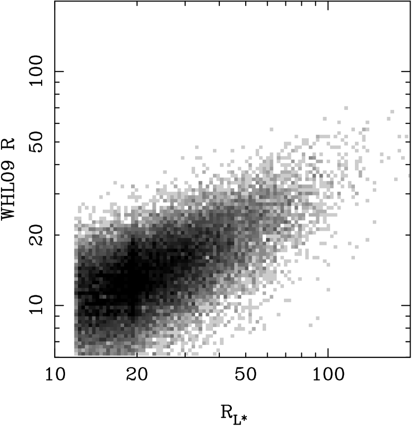
Figure 12.— Same as Figure 10 but between $R$ in WHL09 and $R_{L\ast}$ in this paper.

Matching is applied between two cluster samples in sky coverage of the SDSS DR6. We find that 25,929 (65%) of 39,668 WHL09 clusters are matched with the WHL12 clusters within a separation of $r_{200}$ and a redshift difference of $|\Delta z|\leq 0.05$. Figure 11 shows the matching rate as a function of redshift between the WHL12 clusters and WHL09 clusters. The matching rates of the WHL12 clusters to WHL09 clusters decrease from 85% at $z\sim 0.1$ to 55% at $z\sim 0.4$. The matching rates of the WHL09 clusters to the WHL12 clusters increase from 20% at $z\sim 0.1$ to 40% at $z\sim 0.4$. The matching rates vary as a function of cluster richness within $0.05\leq z<0.42$, 90% of the WHL09 clusters of $R\geq 15$ are matched with the WHL12 clusters, 86% of the WHL12 clusters of $R_{L\ast}\geq 40$ are matched with the WHL09 clusters. If we match the clusters within a separation of $1.5\,r_{200}$, $91\%$ of the WHL09 clusters of $R\geq 15$ are matched. The non-matched WHL09 clusters are probably merged in the friend-of-friend algorithm of our procedure, or are poorer than the criteria of cluster finding in this work.

Figure 12 shows a tight correlation between the WHL09 richness, $R$, and the richness of this paper, $R_{L\ast}$, for the matched clusters.

3.4. Comparison with the GMBCG clusters

Figure 13.— Same as Figure 11 but between the GMBCG clusters and the WHL12 clusters in the sky coverage of the SDSS DR7. The solid lines represent the matching rate within a separation of $r_{200}$ and a redshift difference of $|\Delta z|\leq 0.05$.The dashed lines represent the matching rate within a separation of $1.5\,r_{200}$ and a redshift difference of $|\Delta z|<0.1$.

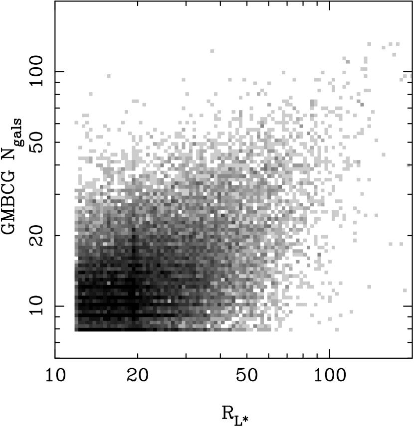
Figure 14.— Same as Figure 10 but between $N_{\rm gal}$ in the GMBCG and $R_{L\ast}$ in this paper.

Hao et al. (2010) presented a GMBCG algorithm, which detects clusters by identifying the red sequence and the BCG feature. From the SDSS DR7, they found 55,424 clusters in the redshift range of $0.1<z<0.55$. They provide two richnesses, the weighted richness which is the total number of galaxies brighter than $0.4L^{\ast}$ within $r_{200}$ weighted by a factor from the fitting of color distribution, and the scaled richness which is the number of galaxies within $r_{200}$ and $2\,\sigma$ of the ridgeline colors. We adopt the weighted richness as GMBCG richness $N_{\rm gals}$ if available, otherwise the scaled richness.

We cross-match the WHL12 clusters with the GMBCG clusters in the sky coverage of the SDSS DR7. We find that 25,370 (46%) of 55,424 GMBCG clusters are matched with the WHL12 clusters within a separation of $r_{200}$ and a redshift difference of $|\Delta z|\leq 0.05$ (see Figure 13). The matching rates of the WHL12 clusters to the GMBCG clusters decrease from 80% at $z\sim 0.1$ to 40% at $z\sim 0.4$. The matching rates of the GMBCG clusters to the WHL12 clusters are 30%–40% within $z<0.4$. Within the redshift range of $0.05\leq z<0.42$, the matching rates increase with cluster richness for both samples. We find that 72% of the GMBCG clusters of $N_{\rm gals}\geq 20$ are matched with the WHL12 clusters, 83% of the WHL12 clusters of $R_{L\ast}\geq 40$ are matched with the GMBCG clusters. The fraction of missing rich GMBCG clusters is larger than those of the maxBCG and WHL09 clusters. This may be due to a broader distribution of redshift difference (see Figure 8). If we match clusters within a separation of $1.5\,r_{200}$ and a redshift difference of $|\Delta z|<0.1$, 55% of the GMBCG clusters are matched with the WHL12 clusters, 85% of the GMBCG rich clusters of $N_{\rm gals}\geq 20$ are matched (see dashed lines in Figure 13).

We note that a few rich GMBCG clusters are still missing. Some of them are merged in the friend-of-friend algorithm of our procedure, or have a redshift difference of $|\Delta z|>0.1$ from the WHL12 clusters. Most of other missing GMBCG clusters are poorer than the criteria of cluster finding in this work. We note a large scatter between the GMBCG richness $N_{\rm gals}$ and $R_{L\ast}$ (see Figure 14).

3.5. Comparison with the AMF clusters

Figure 15.— Same as Figure 13 but between the AMF clusters and the WHL12 clusters in the sky coverage of the SDSS DR6.

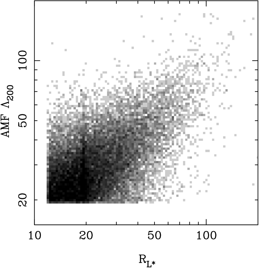
Figure 16.— Same as Figure 10 but between $\Lambda_{200}$ in the AMF and $R_{L\ast}$ in this paper.

Szabo et al. (2011) used a modified AMF algorithm to identify clusters using photometric redshifts of galaxies. From the SDSS DR6, 69,173 clusters are identified in the redshift range $0.045<z<0.78$ with a richness of $\Lambda_{200}\geq 20$. The richness of the AMF clusters is defined as the total luminosity within $r_{200}$ in units of $L^{\ast}$, the same as that in this work.

We cross-match the WHL12 clusters with the AMF clusters in the sky coverage of the SDSS DR6. Within a separation of $r_{200}$ and a redshift difference of $|\Delta z|\leq 0.05$, 27,966 (40%) of 69,173 AMF clusters are matched with the WHL12 clusters. Figure 15 shows the matching rate as a function of redshift. The matching rates of the WHL12 clusters to the AMF clusters decrease from 80% at $z\sim 0.1$ to 30% at $z\sim 0.5$. The matching rates of the AMF clusters to the WHL12 clusters are constantly $\sim$30%. The matching rates vary with cluster richness within $0.05\leq z<0.42$, 72% of the AMF clusters of $\Lambda_{200}\geq 40$ are matched with the WHL12 clusters, 74% of the WHL12 clusters of $R_{L\ast}\geq 40$ are matched with the AMF clusters. We note that many AMF clusters have a large redshift difference of $|\Delta z|>0.05$ (see Figure 8). If we match clusters within a separation of $1.5\,r_{200}$ and a redshift difference of $|\Delta z|<0.1$, 91% of the AMF rich clusters of $\Lambda_{200}\geq 40$ are matched with the WHL12 clusters (see dashed lines in Figure 15). Those non-matched AMF clusters are missing due to friend-of-friend merging of our algorithm, large redshift difference from the WHL12 clusters and large scatter between two richness estimates.

Figure 16 shows the correlation between the AMF richness $\Lambda_{200}$ and the $R_{L\ast}$ for the matched clusters.

3.6. Correlations with X-Ray Measurements

Figure 17.— Correlations between the cluster richness $R_{L\ast}$ with the X-ray luminosity $L_{X}$ (the upper panel) and temperature $T_{X}$ (the bottom panel). The solid lines are the best fits for the correlations. The dashed lines in the upper panel show the $\pm\sigma_{\log L_{X}}$ to the best-fit relation.

With luminous member galaxies well discriminated in the identification procedure, good correlations between the cluster richness with X-ray measurements are expected (Wen et al., 2009).

We get X-ray clusters from the Northern ROSAT All-Sky (NORAS) Galaxy Cluster Survey (Böhringer et al., 2000) and the ROSAT-ESO Flux Limited X-ray (REFLEX) Galaxy cluster survey (Böhringer et al., 2004). The NORAS sample contains 378 clusters and the REFLEX contains 447 clusters. The ROSAT survey provides X-ray luminosity for detected clusters. We also get X-ray clusters from the query of the X-ray Cluster Database (BAX), where luminosities for 1028 clusters and temperatures for 210 clusters are available compiled from reference. The ROSAT clusters mostly are massive with a luminosity greater than $10^{44}~{}{\rm erg~{}s^{-1}}$ in the 0.1–2.4 keV band, while the BAX sample contains many less massive clusters with a low luminosity less than $10^{44}~{}{\rm erg~{}s^{-1}}$. Previous work shows that the luminosity in both samples is statistically consistent (Szabo et al., 2011). Here, we combine two sample for the correlation with our cluster richness. For the clusters in both ROSAT and BAX samples, we adopt the X-ray luminosity from ROSAT data.

X-ray clusters are matched with the WHL12 clusters within a separation of $r_{200}$ and a redshift difference of $|\Delta z|\leq 0.05$. We find 611 matched X-ray clusters with luminosities measured, 84 matched X-ray clusters with temperatures measured. Figure 17 shows the correlations between cluster richness with X-ray luminosity and temperature for the matched clusters. The best fits give

$$\log L_{X,44}=(-2.49\pm 0.16)+(1.59\pm 0.09)\log R_{L\ast},$$ (5)

and

$$\log T_{X}=(-0.43\pm 0.05)+(0.61\pm 0.05)\log R_{L\ast},$$ (6)

where $L_{X,44}$ refers to X-ray luminosity in the 0.1–2.4 keV band in units of $10^{44}~{}{\rm erg~{}s^{-1}}$, $T_{X}$ refers to X-ray temperature in units of keV. The tight correlations suggest that the richness we estimate is reasonable and statistically reliable. The slopes of the $L_{X}$–$R_{L\ast}$ and the $T_{X}$–$R_{L\ast}$ relations are in agreement with those of Szabo et al. (2011). We measure the scatter in X-ray luminosity to the best-fit relation and get a value of $\sigma_{\log L_{X}}=0.38$, i.e., $\sigma_{\ln L_{X}}=0.87$. The scatter is in agreement with that for the correlation of $L_{X}$ with the maxBCG richness (Rykoff et al., 2008), but larger than those for the correlations with the improved maxBCG richness (Rozo et al., 2009b; Rykoff et al., 2012). For a similar comparison, we measure the scatter in cluster mass to the best-fit $M_{200}$–$R_{L\ast}$ relation given in Section 2.2 and get $\sigma_{\log M_{200}}=0.21$, i.e., $\sigma_{\ln M_{200}}=0.48$. The scatter in mass based on our richness is also in agreement with that based on the maxBCG richness (Rozo et al., 2009a).

3.7. Correlations with the SZ Measurements

Figure 18.— Correlations between the cluster richness with the SZ measurement by Planck.

The SZ effect is the result of high energy electrons interacting with the cosmic microwave background radiation through inverse Compton scattering. It has been detected around rich galaxy clusters due to a high temperature of host ionized gas (Carlstrom et al., 1996, 2000). The SZ signal is characterized by the quantity $D^{2}_{A(z)}Y_{\rm SZ}=(\sigma_{T}/m_{e}c^{2})\int PdV$, where $D_{A(z)}$ is the angular distance to a cluster at redshift $z$, $\sigma_{T}$ is the Thomson cross-section, $c$ is the speed of light, $m_{e}$ is the electron rest mass, $\int PdV=\int n_{e}kT_{e}dV$ is the integration of the pressure of hot ionized gas over the cluster volume. As the pressure is related to gravitational potential, $D^{2}_{A(z)}Y_{\rm SZ}$ is expected to be a proxy of cluster mass (Bonamente et al., 2008).

Recently, the Planck releases an SZ cluster sample including 189 clusters (Planck Collaboration et al., 2011). We find that 71 SZ clusters are located at the sky coverage of the SDSS-III. Six of them have redshifts less than 0.05. Other 65 clusters are matched with the WHL12 clusters, of which 61 have X-ray measurements. Figure 18 shows the correlations between the richness and the SZ measurements by the Planck for the 61 clusters, where $Y_{\rm SZ}$ is the SZ signal measured within a radius of $5\,r_{500}$ and $E(z)=\sqrt{\Omega_{\Lambda}+\Omega_{m}(1+z)^{3}}$. The matched clusters mostly have a richness of $R_{L\ast}>50$. Clearly, there is a positive correlation between cluster richness and SZ measurement.

4. BCGs and LRGs in the clusters

BCGs are luminous and usually located at the centers of clusters. Their properties provide the information of galaxy formation in the extreme dense environment. Using our sample, we can study the evolution of the BCGs. Moreover, we cross-identity the BCGs with the SDSS LRG sample.

4.1. Magnitude evolution of the BCGs

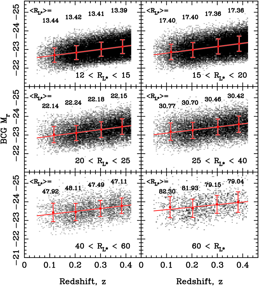
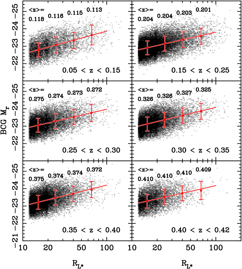
Figure 19.— Upper: evolution of BCG absolute magnitude with cluster redshift in the range of $0.05\leq z<0.42$ for six richness bins. The average absolute magnitudes and the dispersions are plotted for four redshift ranges. The average richnesses are calculated and marked for these redshift ranges. The solid lines show the best-fitting. Lower: correlation between BCG absolute magnitude with cluster richness for six redshift bins. Similarly, the average absolute magnitudes and the dispersions are plotted for four richness ranges, and the average redshifts are marked for these ranges in the plots.
(A color version of this figure is available in the online journal.)

The BCGs in rich clusters are formed at redshift $z>2$ and evolved passively (e.g., Stott et al., 2008). The properties of BCGs are related to their host clusters (Wen & Han, 2011). Richer clusters tend to have brighter BCGs. Here, we use our sample to address the magnitude evolution of the BCGs with redshift and richness.

Figure 19 shows the evolution of absolute magnitudes of the BCGs with cluster redshift in the range of $0.05\leq z<0.42$ for six richness bins and with cluster richness for six redshift bins. We get the mean values and fit the correlation (solid lines) for each bin. Here, the variations of completeness and false detection rate are considered by a weighting factor in the fitting. The weight is calculated as the percentage of true cluster (i.e., $100\%-$false detection rate) divided by completeness for each richness and redshift bin. There are very small changes of the average richnesses within the redshift ranges (upper panels) or the average redshifts within the richness ranges (lower panels), indicating that the changes of BCG magnitudes have been well decoupled for redshift and richness. The best fits between absolute magnitude and redshift give

$$M_{r}=(-22.48\pm 0.01) -(1.74\pm 0.03)z$$

$${\rm for}~{}12<R_{L\ast}<15;$$

$$M_{r}=(-22.63\pm 0.01) -(1.76\pm 0.03)z$$

$${\rm for}~{}15<R_{L\ast}<20;$$

$$M_{r}=(-22.76\pm 0.01) -(1.77\pm 0.05)z$$

$${\rm for}~{}20<R_{L\ast}<25;$$

$$M_{r}=(-22.93\pm 0.01) -(1.66\pm 0.05)z$$

$${\rm for}~{}25<R_{L\ast}<40;$$

$$M_{r}=(-23.17\pm 0.03) -(1.58\pm 0.09)z$$

$${\rm for}~{}40<R_{L\ast}<60;$$

$$M_{r}=(-23.44\pm 0.04) -(1.35\pm 0.17)z$$ (7)

$${\rm for}~{}60<R_{L\ast}.$$

Clearly, the BCG are brighter in clusters of higher redshifts. As the stellar population in the BCGs was formed at redshift $z>2$ and becomes old with comic time, the BCGs become fainter at lower redshifts. To verify the evolution of BCG magnitude with redshift, using the AMF clusters (Szabo et al., 2011) and the brightest one of three BCG candidates for each cluster, we get

$$M_{r,\rm AMF}=(-22.43\pm 0.01)-(1.54\pm 0.04)z,$$ (8)

which is roughly consistent with the results derived from our cluster sample. The BCG magnitude evolution is in agreement with that of $L^{\ast}$ found by Blanton et al. (2003). In addition, we find that BCGs are brighter in richer clusters, consistent with conclusions in previous works (Wen & Han, 2011; Szabo et al., 2011). From the fitting, the BCGs have an average absolute magnitude of $-22.48$ for cluster richness of $R_{L\ast}=12$–15 at redshift $z=0$, but a brighter magnitude of $-23.44$ for cluster richness of $R_{L\ast}>60$. This tendency can be clearly shown from the correlation between BCG absolute magnitude with cluster richness for six redshift bins (the lower panel of Figure 19). The evolution of the BCGs magnitudes with redshift and the dependence of richness can be formulated together as,

$$M_{r}=( - 21.25\pm 0.01)-(1.75\pm 0.03)z$$ (9)

$$- (1.10\pm 0.03)\log R_{L\ast}.$$

4.2. Cross-identification between BCGs and LRGs

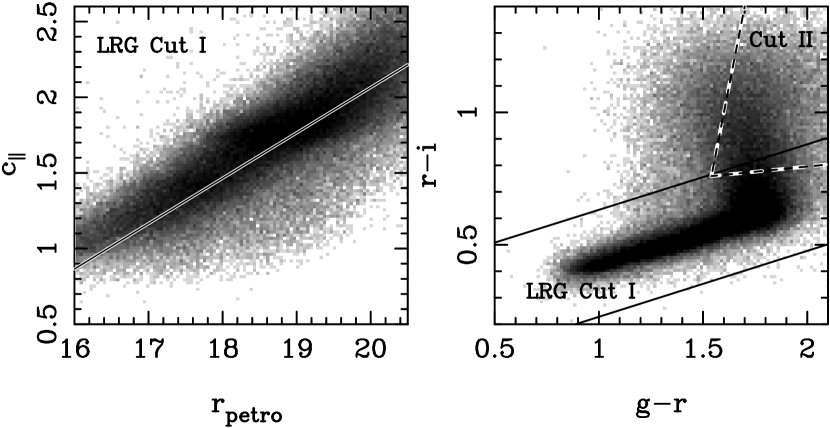
Figure 20.— Color–magnitude and color–color diagrams for BCGs in our clusters. The solid lines represent the color cuts of the SDSS LRG selection.

The SDSS LRGs are selected to produce a volume-limited sample of massive galaxies to redshift of 0.5. They are efficiently selected by color cuts based on passive evolution model at redshifts $z>0.15$ (Eisenstein et al., 2001). Generally, LRGs are more massive and located at denser environment than general galaxies. They are most likely BCGs or brightest group galaxies. BCGs are luminous and mostly have red colors. They are likely to be LRGs. However, this may not always be true. Crawford et al. (1999) showed that about 27% BCGs in X-ray bright clusters have optical emission lines. They may have blue colors due to recent star formation (Hicks et al., 2010; Wang et al., 2010; Pipino et al., 2011). Therefore, many BCGs are not LRGs.

First, we cross-identify the clusters in our sample with the SDSS LRGs to address how many LRGs are member galaxies. We get 112,191 LRGs of $z>0.15$ from the SDSS spectroscopic data. Cross-matching between LRGs with BCGs in our sample, we find that 28,336 (25%) LRGs are BCGs and 40,039 (36%) LRGs are located within a projected separation of $r_{200}$ and a redshift difference of 0.05. This suggests that most LRGs are located not in our clusters but in an environment poorer than our clusters.

On the other hand, we estimate the fraction of the BCGs as the SDSS LRGs. Follow Eisenstein et al. (2001), we match the colors of the BCGs with the LRG selection criteria. Figure 20 shows the color–magnitude and color–color diagrams for the BCGs in our clusters. The color $c_{\parallel}$ is defined as

$$c_{\parallel}=0.7(g-r)+1.2[(r-i)-0.177].$$ (10)

If we only consider the color cuts and do not limit the Petrosian magnitude $r_{\rm petro}$, the BCGs can be classified as LRGs for those with the color $c_{\parallel}$ above the line in the left panel of Figure 20 and the colors, $g-r$ and $r-i$, between the lines in the right panel. There are 83,740 (66%) of 126,041 BCGs in the redshift range $z>0.15$ satisfying the color cuts of the SDSS LRG selection criteria. When the Petrosian magnitude limits of $r_{\rm petro}<19.2$ for Cut I and $r_{\rm petro}<19.5$ for Cut II are considered, we find that 63% of BCGs of $r_{\rm petro}<19.5$ are LRGs.

5. Summary

We identify 132,684 clusters of galaxies in the redshift range $0.05\leq z<0.8$ using photometric redshifts of galaxies from the SDSS-III. The clusters are recognized for those with a richness $R_{L\ast}\geq 12$ and a number of member galaxies candidates $N_{200}\geq 8$ within $r_{200}$. Monte Carlo simulations show that the false detection rate is less than 6% for the whole sample. The cluster detection rate is more than 95% for clusters of $M_{200}>1\times 10^{14}~{}M_{\odot}$ in the redshift range of $0.05\leq z<0.42$. We cross-match our cluster sample with previous cluster samples. The matching rates are 50–70% for previously known clusters but depend on cluster richness. Clusters in our sample match more than 90% of previously known rich clusters. Comparing with X-ray and the Planck data, we find that the determined cluster richness is related to the X-ray luminosity, temperature and SZ measurements. The richer clusters have brighter BCGs. The BCGs are brighter in higher redshift clusters. Cross-matching the BCGs with the SDSS LRGs, we find that 25% LRGs are BCGs of our clusters, 36% LRGs are member galaxies, and 63% of the BCGs of $r_{\rm petro}<19.5$ in our clusters satisfy the SDSS LRG selection criteria.

References

- Abell (1958) Abell, G. O. 1958, ApJS, 3, 211
- Abell et al. (1989) Abell, G. O., Corwin, Jr., H. G., & Olowin, R. P. 1989, ApJS, 70, 1
- Aihara et al. (2011) Aihara, H., et al. 2011, ApJS, 193, 29
- Allen et al. (2011) Allen, S. W., Evrard, A. E., & Mantz, A. B. 2011, ARA&A, 49, 409
- Allen et al. (2008) Allen, S. W., Rapetti, D. A., Schmidt, R. W., Ebeling, H., Morris, R. G., & Fabian, A. C. 2008, MNRAS, 383, 879
- Bahcall (1988) Bahcall, N. A. 1988, ARA&A, 26, 631
- Bahcall et al. (1997) Bahcall, N. A., Fan, X., & Cen, R. 1997, ApJ, 485, L53
- Berlind et al. (2006) Berlind, A. A., et al. 2006, ApJS, 167, 1
- Blain et al. (1999) Blain, A. W., Kneib, J.-P., Ivison, R. J., & Smail, I. 1999, ApJ, 512, L87
- Blanton et al. (2003) Blanton, M. R., et al. 2003, ApJ, 592, 819
- Böhringer et al. (2000) Böhringer, H., et al. 2000, ApJS, 129, 435
- Böhringer et al. (2004) Böhringer, H., et al. 2004, A&A, 425, 367
- Bonamente et al. (2008) Bonamente, M., Joy, M., LaRoque, S. J., Carlstrom, J. E., Nagai, D., & Marrone, D. P. 2008, ApJ, 675, 106
- Butcher & Oemler (1978) Butcher, H. & Oemler, Jr., A. 1978, ApJ, 219, 18
- Butcher & Oemler (1984) —. 1984, ApJ, 285, 426
- Carlberg et al. (1996) Carlberg, R. G., Yee, H. K. C., Ellingson, E., Abraham, R., Gravel, P., Morris, S., & Pritchet, C. J. 1996, ApJ, 462, 32
- Carlstrom et al. (1996) Carlstrom, J. E., Joy, M., & Grego, L. 1996, ApJ, 456, L75
- Carlstrom et al. (2000) Carlstrom, J. E., Joy, M. K., Grego, L., Holder, G. P., Holzapfel, W. L., Mohr, J. J., Patel, S., & Reese, E. D. 2000, Physica Scripta Volume T, 85, 148
- Crawford et al. (1999) Crawford, C. S., Allen, S. W., Ebeling, H., Edge, A. C., & Fabian, A. C. 1999, MNRAS, 306, 857
- Csabai et al. (2007) Csabai, I., Dobos, L., Trencséni, M., Herczegh, G., Józsa, P., Purger, N., Budavári, T., & Szalay, A. S. 2007, Astronomische Nachrichten, 328, 852
- Dahle (2006) Dahle, H. 2006, ApJ, 653, 954
- Dressler (1980) Dressler, A. 1980, ApJ, 236, 351
- Eisenstein et al. (2001) Eisenstein, D. J., et al. 2001, AJ, 122, 2267
- Estrada et al. (2009) Estrada, J., Sefusatti, E., & Frieman, J. A. 2009, ApJ, 692, 265
- Gladders & Yee (2005) Gladders, M. D. & Yee, H. K. C. 2005, ApJS, 157, 1
- Goto et al. (2002) Goto, T., et al. 2002, AJ, 123, 1807
- Goto et al. (2003) Goto, T., Yamauchi, C., Fujita, Y., Okamura, S., Sekiguchi, M., Smail, I., Bernardi, M., & Gomez, P. L. 2003, MNRAS, 346, 601
- Hao et al. (2010) Hao, J., et al. 2010, ApJS, 191, 254
- Hicks et al. (2010) Hicks, A. K., Mushotzky, R., & Donahue, M. 2010, ApJ, 719, 1844
- Hong et al. (2012) Hong, T., Han, J. L., Wen, Z. L., Sun L., & Zhan, H. 2012, ApJ, 749, 81
- Huchra & Geller (1982) Huchra, J. P. & Geller, M. J. 1982, ApJ, 257, 423
- Hütsi (2010) Hütsi, G. 2010, MNRAS, 401, 2477
- Jenkins et al. (2001) Jenkins, A., Frenk, C. S., White, S. D. M., Colberg, J. M., Cole, S., Evrard, A. E., Couchman, H. M. P., & Yoshida, N. 2001, MNRAS, 321, 372
- Koester et al. (2007a) Koester, B. P., et al. 2007a, ApJ, 660, 239
- Koester et al. (2007b) Koester, B. P., et al. 2007b, ApJ, 660, 221
- Lopez et al. (2008) Lopez, S., et al. 2008, ApJ, 679, 1144
- Lupton et al. (2001) Lupton, R., Gunn, J. E., Ivezić, Z., Knapp, G. R., & Kent, S. 2001, in ASP Conf. Ser. 238, Astronomical Data Analysis Software and Systems X, ed. F. R. Harnden, Jr., F. A. Primini, & H. E. Payne(San Francisco, CA:ASP), 269
- Marriage et al. (2011) Marriage, T. A., et al. 2011, ApJ, 737, 61
- Merchán & Zandivarez (2005) Merchán, M. E. & Zandivarez, A. 2005, ApJ, 630, 759
- Metcalfe et al. (2003) Metcalfe, L., et al. 2003, A&A, 407, 791
- Myers et al. (2005) Myers, A. D., Outram, P. J., Shanks, T., Boyle, B. J., Croom, S. M., Loaring, N. S., Miller, L., & Smith, R. J. 2005, MNRAS, 359, 741
- Pedersen & Dahle (2007) Pedersen, K. & Dahle, H. 2007, ApJ, 667, 26
- Pipino et al. (2011) Pipino, A., Szabo, T., Pierpaoli, E., MacKenzie, S. M., & Dong, F. 2011, MNRAS, 417, 2817
- Planck Collaboration et al. (2011) Planck Collaboration, Ade, P. A. R., Aghanim, N., et al. 2011, A&A, 536, A8
- Popesso et al. (2004) Popesso, P., Böhringer, H., Brinkmann, J., Voges, W., & York, D. G. 2004, A&A, 423, 449
- Postman et al. (1992) Postman, M., Huchra, J. P., & Geller, M. J. 1992, ApJ, 384, 404
- Postman et al. (1996) Postman, M., Lubin, L. M., Gunn, J. E., Oke, J. B., Hoessel, J. G., Schneider, D. P., & Christensen, J. A. 1996, AJ, 111, 615
- Reiprich & Böhringer (2002) Reiprich, T. H. & Böhringer, H. 2002, ApJ, 567, 716
- Rines et al. (2007) Rines, K., Diaferio, A., & Natarajan, P. 2007, ApJ, 657, 183
- Rozo et al. (2009a) Rozo, E., et al. 2009a, ApJ, 699, 768
- Rozo et al. (2009b) Rozo, E., et al. 2009b, ApJ, 703, 601
- Rykoff et al. (2008) Rykoff, E. S., et al. 2008, ApJ, 675, 1106
- Rykoff et al. (2012) Rykoff, E. S., et al. 2012, ApJ, 746, 178
- Santos et al. (2004) Santos, M. R., Ellis, R. S., Kneib, J.-P., Richard, J., & Kuijken, K. 2004, ApJ, 606, 683
- Seljak (2002) Seljak, U. 2002, MNRAS, 337, 769
- Smail et al. (2002) Smail, I., Ivison, R. J., Blain, A. W., & Kneib, J.-P. 2002, MNRAS, 331, 495
- Stott et al. (2008) Stott, J. P., Edge, A. C., Smith, G. P., Swinbank, A. M., & Ebeling, H. 2008, MNRAS, 384, 1502
- Stoughton et al. (2002) Stoughton, C., et al. 2002, AJ, 123, 485
- Strauss et al. (2002) Strauss, M. A., et al. 2002, AJ, 124, 1810
- Szabo et al. (2011) Szabo, T., Pierpaoli, E., Dong, F., Pipino, A., & Gunn, J. 2011, ApJ, 736, 21
- Wang et al. (2010) Wang, J., Overzier, R., Kauffmann, G., von der Linden, A., & Kong, X. 2010, MNRAS, 401, 433
- Wen & Han (2011) Wen, Z. L. & Han, J. L. 2011, ApJ, 734, 68
- Wen et al. (2011) Wen, Z. L., Han, J. L., & Jiang, Y. Y. 2011, Res. Astron. Astrophys., 11, 1185
- Wen et al. (2009) Wen, Z. L., Han, J. L., & Liu, F. S. 2009, ApJS, 183, 197
- Wen et al. (2010) —. 2010, MNRAS, 407, 533
- Yang et al. (2005) Yang, X., Mo, H. J., van den Bosch, F. C., & Jing, Y. P. 2005, MNRAS, 356, 1293
- York et al. (2000) York, D. G., et al. 2000, AJ, 120, 1579