Momentum-carrying waves
on D1-D5 microstate geometries
Samir D. Mathur and David Turton
Department of Physics,
The Ohio State University,
Columbus, OH 43210, USA
mathur@mps.ohio-state.edu
turton.7@osu.edu
Abstract
If one attempts to add momentum-carrying waves to a black string then the solution develops a singularity at the horizon; this is a manifestation of the ‘no hair theorem’ for black objects. However individual microstates of a black string do not have a horizon, and so the above theorem does not apply. We construct a perturbation that adds momentum to a family of microstates of the extremal D1-D5 string. This perturbation is analogous to the ‘singleton’ mode localized at the boundary of ; to leading order it is pure gauge in the interior of the geometry.
1 Introduction
One of the great successes of string theory is its ability to reproduce the Bekenstein-Hawking entropy of black holes from a microscopic count of states [1, *Sen:1995in, 3, *Callan:1996dv]. To resolve the information paradox [5, *Hawking:1976ra] however, we need to go beyond indirect counting and understand the gravitational description of individual black hole microstates.
An early attempt to find such ‘black hole hair’ was the construction of solutions describing travelling waves on a heterotic black string [7, 8, *Tseytlin:1996as, *Tseytlin:1996qg], and a D1-D5 black string [11, *Horowitz:1996cj]. In each case the solution had a horizon. It turned out that adding the wave led to curvature singularities at the horizon in the form of infinite tidal forces [13, *Horowitz:1997si] (see also [15, 16]). One could regard this as an instance of the ‘no-hair theorem’: there are no regular perturbations of a horizon.
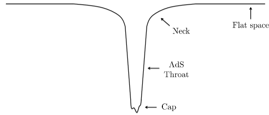
It turns out however that individual states of the D1-D5 system do not have a traditional horizon. The simplest states are described by a semiclassical geometry with an AdS throat ending in a smooth cap [17, 18, 19, *Kanitscheider:2007wq, *Skenderis:2008qn]. This structure is depicted in Fig. 1 and described below. Since there is no horizon, we can ask the question: is there a perturbation of such D1-D5 geometries that is regular and carries momentum along the direction of the D1-D5 string?
In this paper we take a particular class of D1-D5 microstate geometries, and give explicitly a perturbation that adds such momentum. The perturbation involves the directions along the compact torus , and is thus the analog of the ‘internal direction perturbations’ that were studied in [7, 8, *Tseytlin:1996as, *Tseytlin:1996qg, 11, *Horowitz:1996cj]. But since there is no horizon in the D1-D5 microstate, we evade the curvature singularity found in earlier works.
We work in type IIB string theory on . We wrap D1 branes on and D5 branes on , creating a D1-D5 bound state. If we take the radius to be the largest scale in the system, the background D1-D5 geometry has a long throat (Fig. 1).
In this limit the D1-D5 bound state is described by a low energy 1+1 dimensional CFT. This CFT has an ‘orbifold point’ in moduli space [22] that is the analog of a ‘zero coupling’ point for the theory. At the orbifold point the CFT is a sigma model with target space , where .
The gravity perturbations we construct have a simple interpretation in the CFT: they describe excitations of the currents in the CFT which arise from translation symmetry along the four directions of the . (These currents were studied in [23].)
At the orbifold point these currents have a simple expression in terms of the bosonic fields. The orbifold CFT is a symmetrized product of copies of a CFT with target space . Let us label the different copies by an index . Each copy has a bosonic oscillator for each of the four directions of the ; thus we have oscillator modes with . In terms of these modes, the currents are given by
Thus the perturbations we construct are the simplest excitations when considered from the viewpoint of the orbifold CFT: they are just the gravitational dual of a single bosonic oscillator mode (symmetrized among all the copies).
For concreteness we first work with the simplest D1-D5 ground state – the one with highest spin, which we denote by . The geometry sourced by is known [24, 25]. We construct the dual perturbation for the CFT state
Denoting the background metric and RR 2-form by , the state is described by perturbed fields . We obtain these perturbations .
In a recent paper [26] approximate forms of were found in two different regions of the geometry sourced by ; matching in the overlap region was used to argue that a complete perturbation of the desired form should exist. In this paper we find the full in closed form and extend the construction to a larger class of background geometries.
Let us discuss the form expected of the perturbation. By the general ideas of Brown and Henneaux [27], the gravity duals of symmetry currents should be given by pure diffeomorphisms in an asymptotically geometry.111These ideas have been used by Strominger [28] and extended to a set of principles for general black holes by Carlip [29, *Carlip:1999cy, *Carlip:1999db]. Thus for each currents, the gravity perturbation should be a diffeomorphism (created by translations) in the ‘throat’ region of the geometry in Fig. 1. But the perturbation cannot be a pure diffeomorphism everywhere, since the corresponding CFT excitation adds an energy to the state . We will observe that the perturbation we construct reduces to a diffeomorphism inside the ‘throat’ region of the geometry, but is not a diffeomorphism in the ‘neck’ (which is, in a sense, the boundary of the region).
Having the perturbation in closed form also permits us to examine it in a very different limit – one in which is the smallest scale in the system, rather than the largest. In this limit the background D1-D5 geometry has the shape of a ring. Interestingly, we find that the perturbation has structure over the entire region spanned by the ring (instead of being confined to the thickness of the ring).
Finally, we extend the construction of the perturbation to a larger family of D1-D5 ground states – the family of all D1-D5 ground states having symmetry [24, 25]. The energy of the gravity perturbation in each case agrees with the excitation energy expected for the corresponding CFT state.
This paper is organized as follows. In Section 2 we introduce the background geometry created by and the operator in the D1-D5 CFT. In Section 3 we give the perturbation and analyze its properties. In Section 4 we generalize the perturbation to the larger class of background geometries. In Section 5 we discuss our results and future directions.
2 The background and the perturbation
2.1 The background geometry
We work with type IIB string theory with the compactification
| (2.1) |
We wrap D1 branes on , D5 branes on , and consider the bound states of these branes. The fermions in the theory are periodic around the , so the dimensional CFT in the directions is in the Ramond sector around the circle.
This D1-D5 system is U-dual to an NS1-P system, where the D5 branes become a multiwound fundamental string along the and the D1 branes become momentum P carried as travelling waves on the string. The gravitational solution of such a string carrying waves is well known [32, *Callan:1995hn, *Dabholkar:1995nc, 17], and may be dualized back to obtain gravitational solutions describing the D1-D5 bound states [17, 18]. We use the light-cone coordinates
| (2.2) |
constructed from the time and coordinate . The different vibration profiles of the NS1P solutions leads to each D1-D5 solution being characterized by such a profile .
The generic state in this system is quantum in nature and the gravitational field it sources is not well-described by a classical geometry. This is simply because the momentum on the NS1 is spread over many different harmonics, with an occupation number of order unity per harmonic. One can however gain insight into the physics of generic solutions by starting with special ones, where all the momentum is placed in a few harmonics. In this case one can take coherent states for the vibrating NS1 string, which are then described by a classical profile function and which source classical geometries [35].
2.2 The long AdS throat limit
As mentioned above, we will be interested in taking a limit of parameters where the geometry has the form depicted in Fig. 1, where we have a long ‘throat’ region where the geometry is locally . To take this limit, we take to be large compared to :
| (2.9) |
We take small enough that we get several units of the radius between the cap and the neck.
The different parts of the geometry (2.6) then have the following structure (Fig. 1) which is generic for two-charge geometries:
-
(i)
For we have approximately flat space.
-
(ii)
At we have the intermediate ‘neck’ region.
-
(iii)
For we have the ‘throat’, which is locally .
-
(iv)
At we have the ‘cap’.
In the case of the background (2.6), the cap is global . We refer to the combined throat+cap as the ‘inner region’. If one decouples the inner region completely from the rest of the geometry, one obtains an asymptotically geometry which is dual to a 1+1 dimensional CFT.
2.3 currents in the D1-D5 orbifold CFT
The D1-D5 bound state is described in the IR limit by a 1+1 dimensional sigma model, with base space and target space a deformation of the orbifold , the symmetric product of copies of . The CFT has supersymmetry, and a moduli space which preserves this supersymmetry. It is conjectured that in this moduli space there is an ‘orbifold point’ where the target space is just the orbifold [22].
The CFT with target space just one copy of is described by four real bosons , four left-moving fermions and four right-moving fermions . The central charge is . The complete theory with target space has copies of this CFT, with states that are symmetrized between the copies. The orbifolding also generates ‘twist’ sectors, which will be relevant later in this paper.
We use to label different copies of the CFT. At the orbifold point we note that each copy has four holomorphic currents
| (2.10) |
arising from translations in the four torus directions. The total CFT then has the currents
| (2.11) |
The modes of the current are then simply the bosonic oscillator modes , and the modes of are
| (2.12) |
Based on the work of Brown and Henneaux [27], the gravity dual of
| (2.13) |
should be a perturbation around the geometry (2.6), with the property that in the throat it reduces to a diffeomorphism. At the boundary of the region, the diffeomorphism should simply be that of a translation along the direction , as a function of [26]. In the next section we describe a perturbation with exactly these properties.
2.4 The field equations for the perturbation
We consider a perturbation given by the fields
| (2.14) |
where is a small parameter. From now on we single out a particular direction in the torus to work with,
| (2.15) |
and take the perturbation to be given by
| (2.16) |
To linear order in the perturbation, we have , so that the Ricci scalar vanishes. The equations for the perturbation are obtained from linearizing about the background the 10D equations ()
| (2.17) | |||||
| (2.18) |
We write
| (2.19) |
Then we find , and the Einstein equation (2.17) reduces to
| (2.20) |
The field equation (2.18) gives
| (2.21) |
where the terms on the RHS arise from the connection term in the covariant derivatives. The equations (2.20), (2.21) can be separated by writing
| (2.22) |
Following [26] we work in an ansatz where we set
| (2.23) |
which gives and leaves us with the equation
| (2.24) |
3 The perturbation and its properties
3.1 The perturbation
We now present a perturbation which solves the linearized equations of motion (2.24) on the background (2.6). The perturbation is given by the following fields:
| (3.1) | |||||
| (3.2) | |||||
| (3.3) | |||||
and
| (3.4) |
In the following section we will comment on the properties of this perturbation. In the perturbation, takes the values
| (3.5) |
After quantization, negative values of will correspond to annihilation operators for the same modes that are described by positive (see [26] for a more detailed discussion). The case describes a deformation that carries charge; these charges were considered in [23] but we will not focus on such solutions here.
We now comment on how this perturbation was derived. In [26], an approximate construction of this perturbation was made following a method developed in [37]. The method involves taking two limits of the background geometry, the ‘outer region’ given by and the ‘inner region’ given by .
The equations of motion may be solved in the two limits and the solutions matched in the region of overlap . In [26], this procedure was followed to first order in this approximation scheme. By following the procedure to higher orders, and demanding a regular solution at each order, one is led to the above closed-form solution.
3.2 Properties of the perturbation
In Section 2.2 we noted that when we take then we get a ‘long AdS throat’. In this regime of parameters, we will see that the perturbation (3.3) has the following properties. The perturbation:
-
(i)
is normalizable at infinity;
-
(ii)
reduces to being a pure diffeomorphism in the throat+cap to leading order;
-
(iii)
is not pure gauge everywhere;
-
(iv)
is smooth in the ‘cap’ region;
-
(v)
has the correct spacetime dependence to carry the energy and momentum
required by the excitation .
We shall demonstrate (i), (ii) and (iv) explicitly; the other properties are easily verified.
3.2.1 Normalizablility at infinity
We first show that the perturbation is normalizable at infinity by examining the stress-energy tensor for the reduced gauge field , where were defined in (2.19). To do this we examine the fall-off of , the component of the stress-energy tensor.
The background falls off as as in an orthonormal frame. Its coupling to the field then contributes at subleading order in and so to leading order at infinity the stress-energy tensor is that of a normal gauge field,
| (3.6) |
We then find that
| (3.7) |
Integrating over the remaining space directions then gives
| (3.8) |
so we see that the perturbation is normalizable at infinity.
3.2.2 Throat+cap region of background
In order to show properties (ii) and (iv), we take the throat+cap limit of the background. This is obtained by taking the limit
| (3.9) |
in the full geometry (2.6). Recall that we have taken . In the limit (3.9) we have .
The background metric (2.6) is singular when , which occurs when and . To show that the fields are regular at we must first change to coordinates in which the background is smooth at . We thus make the spectral flow [38, 24, 25] transformation to the NS coordinates
| (3.10) |
We then make the change of coordinates
| (3.11) |
under which the 10D throat+cap metric becomes global :
| (3.12) |
where is the metric on a round unit .
3.2.3 Pure gauge to leading order in the throat+cap
We first show that to leading order in the throat+cap, the perturbation reduces to being a pure diffeomorphism accompanied by a gauge transformation
| (3.13) |
When we go to a unit orthonormal frame, we find that the components are smaller than the other nonvanishing components by a factor . Thus we ignore these components, leaving
| (3.14) | |||||
| (3.15) |
The gauge field also has two nontrivial components, since
| (3.16) |
We now observe that the above metric and gauge field perturbations (3.15), (3.16) are generated by a diffeomorphism with parameter and a gauge transformation with parameter , where
| (3.17) | |||||
| (3.18) |
The upper region of the throat, given by , is analogous to the region near the boundary of after decoupling the throat from the flat asymptotics. We next observe that in this region, to leading order the above diffeomorphism becomes a translation in the direction as a function of only:
| (3.19) |
As shown in [26], this connects this perturbation, via the work of Brown and Henneaux, to the current .
3.2.4 Smoothness at the origin
To show that the fields are smooth at the origin, we make the diffeomorphism with parameter and gauge transformation with parameter given by
| (3.20) | |||||
| (3.21) |
This removes the pure gauge part of the perturbation described above, including the component in (3.3) which appeared potentially singular at . We next take the cap limit
| (3.22) |
and spectral flow to NS coordinates using (3.10). This gives the cap fields
| (3.23) | |||||
| (3.24) | |||||
| (3.25) | |||||
and
It can be checked that these fields are smooth at .
3.3 Perturbation in the black ring limit
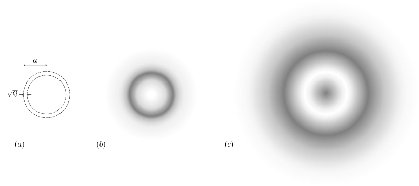
In the above discussion we had taken the radius large compared to the curvature scale of the geometry: . In this limit the solution (2.6) takes the form depicted in Fig. 1. But we can also take the opposite limit: . In this limit the geometry (2.6) becomes a ring, depicted in Fig. 2 (a). The ring has a ‘thickness’ , and a radius . The metric is nontrivial within the thickness of the ring, and goes over to flat space when the distance from the ring axis becomes much larger than .
Since the perturbation (3.3) that we have constructed is given in closed form as a function of , we can examine it in the ring limit as well. A priori, we would anticipate one of two possibilities: (i) the perturbation may be confined to the ring thickness, dying away at distances much larger than from the ring axis (ii) the perturbation spreads over a much larger region of the size of the ring itself, controlled by the scale .
For comparison, in [39] a momentum-carrying perturbation of the D1-D5 background (2.6) was studied, obtaining a microstate of the D1-D5-P black ring [40, *Elvang:2004ds]. In that case the perturbation was of type (i). We depict this in Fig. 2 (b). Interestingly, in the present case we find that our perturbation is of type (ii). To see this, note that the hierarchy of scales is now
| (3.26) |
Consider for example :
| (3.27) |
At the axis of the ring, we have , and we see that near this location the perturbation vanishes as . In fact the perturbation grows up to the scale before eventually falling off as . So we see the perturbation does not have its main structure inside the ‘tube’ but has structure on the scale of the ring itself. We depict this in Fig. 2 (c).
The source of the difference between the two cases can be traced to the following fact. In the case studied in [39] the perturbation had a wavenumber along the long axis of the ring, and by taking large one obtained a perturbation that fell off rapidly outside the thickness of the ring. Our present perturbation has no oscillations along the ring axis; thus increasing the level of does not give us a high wavenumber along the ring. So the perturbation for the are analogous to the small case of [39]. For small the perturbation of [39] also spread over the scale of the entire ring.
4 Extension to a larger class of backgrounds
4.1 The perturbation on conical defect metrics
We have so far worked with the background sourced by , the Ramond ground state which is the spectral flow of the NS vacuum of the D1-D5 CFT. This geometry is one of a family of D1-D5 geometries studied in [24, 25]. This family is characterized by a parameter
| (4.1) |
The case corresponds to the state which is described by the solution (2.6). The other members of the family are obtained in the CFT by acting on with twist operators, for details see [18]. The resulting states have ‘component strings’ of winding number each; each component string is generated by the action of a twist operator that twists together copies of the CFT.
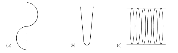
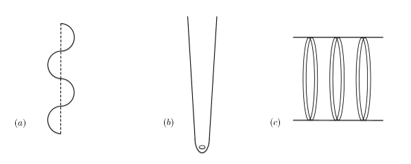
We have seen that the gravitational solution for and has a smooth cap which is global . For however, the geometries have conical singularities. This is related to the fact that these solutions are U-dual to an NS1-P profile which runs over itself times. In Fig. 3 and Fig. 4 we qualitatively sketch the cases and . In each figure, we first sketch the U-dual NS1-P profile, then the throat+cap region of the corresponding D1-D5 geometry, and finally the dual orbifold CFT state.
4.2 Derivation of the generalization
When the ‘throat+cap’ of the solution (4.2) is an orbifold of (we ignore the for this discussion). This can be seen as follows. The throat+cap region is obtained by setting , which gives . In this limit the metric (4.2) is
| (4.8) | |||||
The metric can be diagonalized by introducing the coordinates
| (4.9) |
in terms of which the metric becomes
| (4.10) |
which is (locally) the metric of . However, note that the identifications on the initial variables were
| (4.11) |
In the new variables, these become
| (4.12) |
where the first identification has a joint displacement of both and . This identification has a fixed point where both the and circles collapse to zero size, which happens at . This is just the curve in the geometry (4.2). Thus this curve (which has the shape of a circle) is the location of an orbifold singularity. The singularity is a conical defect created by identifying an angular variable by instead of by .
Since the metric (4.10) has the same form as in the case , we can locally solve the equations of motion by the perturbation (3.3) that we had for the case . The change of coordinates implies that the functions in the perturbation will come with factors of the form
| (4.13) |
We now rewrite this expression in the original coordinates of the metric (4.2), getting
| (4.14) |
At infinity the momentum along must be quantized in units of , so we must impose
| (4.15) |
Then (4.14) becomes
| (4.16) |
where we have written the power on the dependence in terms of as before. Substituting this expression and replacing where appropriate in (3.3) gives the generalized perturbation (4.7). We have verified that (4.7) solves the perturbation equations around the metric (4.2).
4.3 The CFT excitation
Let us look at the excitation in the orbifold CFT corresponding to the perturbation (4.7). We imagine quantizing the mode (4.7), and taking a single quantum of the perturbation. The quantum has energy , which corresponds to an excitation at level in the CFT. Since we have a single supergravity quantum, we expect that only one component string will be excited (see [18] for more details on relating gravity quanta to CFT excitations).
Denoting the Ramond vacuum of the th component string by , the perturbation in the CFT with these characteristics is given by
| (4.17) |
Here we have a single bosonic oscillator in mode on one of the component strings (and we have symmetrized over all the component strings). Since the CFT with twisted cycles lives in a ‘box’ of length , the oscillator at level carries energy , as desired.
Note that there are many other states possible at this energy level, since we are at level on the twisted component string. Construction of the other states at this level is a more complicated task, which we hope to address elsewhere.
5 Discussion
The gravitational description of all two-charge D1-D5 states can be understood. This is possible because the D1-D5 system can be mapped by dualities to NS1-P, which is a string carrying travelling waves. The metrics for such strings are known [32, *Callan:1995hn, *Dabholkar:1995nc, 17], and dualizing back we get the metrics for D1-D5 bound states [17, 18]. There is however no known construction which gives all three-charge D1-D5-P solutions in a similar way. Instead, families of D1-D5-P states have been constructed by diverse methods [42, *Jejjala:2005yu, 44, *Balasubramanian:2006gi, *Bena:2007kg, *Bena:2011uw, 48, *Giusto:2012gt, *Vasilakis:2012zg]. In some cases, the gravity solutions have been identified with their counterparts in the orbifold CFT.
In this paper we have taken a particular set of CFT states and constructed their gravity duals. These states are special in the following sense. Recall that the CFT on D3 branes is gauge theory, which splits into an factor (dual to [51]) and a factor which is dual to a singleton [52, *Flato:1978qz] mode localized at the ‘boundary of ’ [54]. Similarly, in the D1-D5 case we have modes localized at the boundary of [55, 56] which are dual to CFT excitations created by the chiral algebra of the CFT. In particular the chiral currents generate such boundary modes, which we have studied in the present paper.
The background we work with is not, however, the space but the entire asymptotically flat geometry sourced by the D1 and D5 branes. Here the boundary of is naturally bounded by a ‘neck’ region that leads to the asymptotically flat part of spacetime. Following the general arguments of Brown and Henneaux, we expect the singleton mode to be a diffeomorphism in the region. We find that our perturbation is pure gauge to leading order in the region, and nontrivial in the neck; this allows it to carry the required energy of the CFT excitation.
The black string waves of [7, 8, *Tseytlin:1996as, *Tseytlin:1996qg, 11, *Horowitz:1996cj] were found to be singular at the horizon; the same was found of the corresponding modes in [15] when examined at quadratic order [16]. In our case the perturbation is given by smooth functions on a smooth geometry with no horizon, so we do not expect any such singularity.
The state in the orbifold CFT corresponding to this perturbation is the simplest possible excitation in the CFT. The orbifold CFT has (on each of the copies) four free bosons and four free fermions. The perturbation we have constructed corresponds to exciting one bosonic oscillator mode (symmetrized over the copies of the CFT).
It is interesting to compare the CFT excitation for with the excitation that corresponds to the Virasoro generators . In terms of the bosonic oscillators of the th copy of the CFT, is given by
| (5.1) |
while is given by
| (5.2) |
Note however that acting twice with is very different from acting with , since
| (5.3) |
so that we have a very different correlation between the ‘copy index’ of the two oscillators. This difference is analogous to the difference in the D3 brane case between the operators and .
Our solutions are new three-charge perturbations, which depend on the light-cone coordinate . They are not generated by simply adding a wave to the background geometry in the way we add a wave to a string. The latter approach needs a null Killing vector along which we must translate [32], and there is no such Killing vector for the background D1-D5 microstate solution (2.6). Instead, there is a detailed structure of the perturbation in the cap region which ensures its regularity.
There are many possible directions in which to continue this research. One is to construct the perturbation in this paper to quadratic order, and potentially to a fully nonlinear solution. Another possible direction is to generalize the construction of this paper to other background geometries, for example known classes of three-charge extremal and non-extremal solutions [42, *Jejjala:2005yu]. It would also be interesting to see how our solutions relate to the analysis of [57].
Acknowledgements
We thank Steve Carlip, Atish Dabholkar, Stefano Giusto, Murat Gunaydin, Dileep Jatkar, Rodolfo Russo and Yogesh Srivastava for helpful discussions. This work was supported in part by DOE grant DE-FG02-91ER-40690.
References
- [1] L. Susskind, “Some speculations about black hole entropy in string theory,” hep-th/9309145
- [2] A. Sen, “Extremal black holes and elementary string states,” Mod. Phys. Lett. A10 (1995) 2081–2094, hep-th/9504147
- [3] A. Strominger and C. Vafa, “Microscopic Origin of the Bekenstein-Hawking Entropy,” Phys. Lett. B379 (1996) 99–104, hep-th/9601029
- [4] C. G. Callan and J. M. Maldacena, “D-brane Approach to Black Hole Quantum Mechanics,” Nucl. Phys. B472 (1996) 591–610, hep-th/9602043
- [5] S. W. Hawking, “Particle Creation by Black Holes,” Commun. Math. Phys. 43 (1975) 199–220
- [6] S. W. Hawking, “Breakdown of Predictability in Gravitational Collapse,” Phys. Rev. D14 (1976) 2460–2473
- [7] F. Larsen and F. Wilczek, “Internal Structure of Black Holes,” Phys. Lett. B375 (1996) 37–42, hep-th/9511064
- [8] M. Cvetic and A. A. Tseytlin, “Solitonic strings and BPS saturated dyonic black holes,” Phys. Rev. D53 (1996) 5619–5633, hep-th/9512031
- [9] A. A. Tseytlin, “Extreme dyonic black holes in string theory,” Mod.Phys.Lett. A11 (1996) 689–714, hep-th/9601177
- [10] A. A. Tseytlin, “Extremal black hole entropy from conformal string sigma model,” Nucl.Phys. B477 (1996) 431–448, hep-th/9605091
- [11] G. T. Horowitz and D. Marolf, “Counting states of black strings with traveling waves,” Phys. Rev. D55 (1997) 835–845, hep-th/9605224
- [12] G. T. Horowitz and D. Marolf, “Counting states of black strings with traveling waves. II,” Phys. Rev. D55 (1997) 846–852, hep-th/9606113
- [13] N. Kaloper, R. C. Myers, and H. Roussel, “Wavy strings: Black or bright?,” Phys. Rev. D55 (1997) 7625–7644, hep-th/9612248
- [14] G. T. Horowitz and H.-s. Yang, “Black strings and classical hair,” Phys. Rev. D55 (1997) 7618–7624, hep-th/9701077
- [15] N. Banerjee, I. Mandal, and A. Sen, “Black Hole Hair Removal,” JHEP 07 (2009) 091, 0901.0359
- [16] D. P. Jatkar, A. Sen, and Y. K. Srivastava, “Black Hole Hair Removal: Non-linear Analysis,” JHEP 02 (2010) 038, 0907.0593
- [17] O. Lunin and S. D. Mathur, “Metric of the multiply wound rotating string,” Nucl. Phys. B610 (2001) 49–76, hep-th/0105136
- [18] O. Lunin and S. D. Mathur, “AdS/CFT duality and the black hole information paradox,” Nucl. Phys. B623 (2002) 342–394, hep-th/0109154
- [19] O. Lunin, J. M. Maldacena, and L. Maoz, “Gravity solutions for the D1-D5 system with angular momentum,” hep-th/0212210
- [20] I. Kanitscheider, K. Skenderis, and M. Taylor, “Fuzzballs with internal excitations,” JHEP 06 (2007) 056, 0704.0690
- [21] K. Skenderis and M. Taylor, “The fuzzball proposal for black holes,” Phys. Rept. 467 (2008) 117–171, 0804.0552
- [22] N. Seiberg and E. Witten, “The D1/D5 system and singular CFT,” JHEP 04 (1999) 017, hep-th/9903224
- [23] F. Larsen and E. J. Martinec, “U(1) charges and moduli in the D1-D5 system,” JHEP 06 (1999) 019, hep-th/9905064
- [24] V. Balasubramanian, J. de Boer, E. Keski-Vakkuri, and S. F. Ross, “Supersymmetric conical defects: Towards a string theoretic description of black hole formation,” Phys. Rev. D64 (2001) 064011, hep-th/0011217
- [25] J. M. Maldacena and L. Maoz, “De-singularization by rotation,” JHEP 12 (2002) 055, hep-th/0012025
- [26] S. D. Mathur and D. Turton, “Microstates at the boundary of AdS,” 1112.6413
- [27] J. D. Brown and M. Henneaux, “Central Charges in the Canonical Realization of Asymptotic Symmetries: An Example from Three-Dimensional Gravity,” Commun. Math. Phys. 104 (1986) 207–226
- [28] A. Strominger, “Black hole entropy from near-horizon microstates,” JHEP 02 (1998) 009, hep-th/9712251
- [29] S. Carlip, “Black hole entropy from conformal field theory in any dimension,” Phys. Rev. Lett. 82 (1999) 2828–2831, hep-th/9812013
- [30] S. Carlip, “Entropy from conformal field theory at Killing horizons,” Class. Quant. Grav. 16 (1999) 3327–3348, gr-qc/9906126
- [31] S. Carlip, “Black hole entropy from horizon conformal field theory,” Nucl. Phys. Proc. Suppl. 88 (2000) 10–16, gr-qc/9912118
- [32] D. Garfinkle and T. Vachaspati, “Cosmic string traveling waves,” Phys.Rev. D42 (1990) 1960–1963
- [33] C. G. Callan, J. M. Maldacena, and A. W. Peet, “Extremal Black Holes As Fundamental Strings,” Nucl. Phys. B475 (1996) 645–678, hep-th/9510134
- [34] A. Dabholkar, J. P. Gauntlett, J. A. Harvey, and D. Waldram, “Strings as Solitons & Black Holes as Strings,” Nucl. Phys. B474 (1996) 85–121, hep-th/9511053
- [35] S. D. Mathur, “The fuzzball proposal for black holes: An elementary review,” Fortsch. Phys. 53 (2005) 793–827, hep-th/0502050
- [36] M. Cvetic and D. Youm, “General Rotating Five Dimensional Black Holes of Toroidally Compactified Heterotic String,” Nucl. Phys. B476 (1996) 118–132, hep-th/9603100
- [37] S. D. Mathur, A. Saxena, and Y. K. Srivastava, “Constructing ’hair’ for the three charge hole,” Nucl. Phys. B680 (2004) 415–449, hep-th/0311092
- [38] A. Schwimmer and N. Seiberg, “Comments on the N=2, N=3, N=4 Superconformal Algebras in Two-Dimensions,” Phys.Lett. B184 (1987) 191
- [39] S. Giusto, S. D. Mathur, and Y. K. Srivastava, “A microstate for the 3-charge black ring,” Nucl. Phys. B763 (2007) 60–90, hep-th/0601193
- [40] H. Elvang, R. Emparan, D. Mateos, and H. S. Reall, “A Supersymmetric black ring,” Phys.Rev.Lett. 93 (2004) 211302, hep-th/0407065
- [41] H. Elvang, R. Emparan, D. Mateos, and H. S. Reall, “Supersymmetric black rings and three-charge supertubes,” Phys.Rev. D71 (2005) 024033, hep-th/0408120
- [42] S. Giusto, S. D. Mathur, and A. Saxena, “Dual geometries for a set of 3-charge microstates,” Nucl. Phys. B701 (2004) 357–379, hep-th/0405017
- [43] V. Jejjala, O. Madden, S. F. Ross, and G. Titchener, “Non-supersymmetric smooth geometries and D1-D5-P bound states,” Phys. Rev. D71 (2005) 124030, hep-th/0504181
- [44] I. Bena and N. P. Warner, “One ring to rule them all … and in the darkness bind them?,” Adv. Theor. Math. Phys. 9 (2005) 667–701, hep-th/0408106
- [45] V. Balasubramanian, E. G. Gimon, and T. S. Levi, “Four Dimensional Black Hole Microstates: From D-branes to Spacetime Foam,” JHEP 01 (2008) 056, hep-th/0606118
- [46] I. Bena and N. P. Warner, “Black holes, black rings and their microstates,” Lect. Notes Phys. 755 (2008) 1–92, hep-th/0701216
- [47] I. Bena, J. de Boer, M. Shigemori, and N. P. Warner, “Double, Double Supertube Bubble,” JHEP 10 (2011) 116, 1107.2650
- [48] S. Giusto, R. Russo, and D. Turton, “New D1-D5-P geometries from string amplitudes,” JHEP 11 (2011) 062, 1108.6331
- [49] S. Giusto and R. Russo, “Adding new hair to the 3-charge black ring,” 1201.2585
- [50] O. Vasilakis, “Bubbling the Newly Grown Black Ring Hair,” 1202.1819
- [51] J. M. Maldacena, “The large N limit of superconformal field theories and supergravity,” Adv. Theor. Math. Phys. 2 (1998) 231–252, hep-th/9711200
- [52] P. A. Dirac, “A Remarkable respresentation of the 3+2 de Sitter group,” J.Math.Phys. 4 (1963) 901–909
- [53] M. Flato and C. Fronsdal, “One Massless Particle Equals Two Dirac Singletons: Elementary Particles in a Curved Space. 6,” Lett. Math. Phys. 2 (1978) 421–426
- [54] E. Witten, “Anti-de Sitter space and holography,” Adv. Theor. Math. Phys. 2 (1998) 253–291, hep-th/9802150
- [55] M. Gunaydin, G. Sierra, and P. K. Townsend, “The Unitary Supermultiplets of D = 3 Anti-De Sitter and D = 2 Conformal Superalgebras,” Nucl. Phys. B274 (1986) 429
- [56] J. de Boer, “Six-dimensional supergravity on S**3 x AdS(3) and 2d conformal field theory,” Nucl. Phys. B548 (1999) 139–166, hep-th/9806104
- [57] I. Bena, S. Giusto, M. Shigemori, and N. P. Warner, “Supersymmetric Solutions in Six Dimensions: A Linear Structure,” 1110.2781