Repulsive Casimir and Casimir-Polder Forces

Abstract

Casimir and Casimir-Polder repulsion have been known for more than 50 years. The general “Lifshitz” configuration of parallel semi-infinite dielectric slabs permits repulsion if they are separated by a dielectric fluid that has a value of permittivity that is intermediate between those of the dielectric slabs. This was indirectly confirmed in the 1970s, and more directly by Capasso’s group recently. It has also been known for many years that electrically and magnetically polarizable bodies can experience a repulsive quantum vacuum force. More amenable to practical application are situations where repulsion could be achieved between ordinary conducting and dielectric bodies in vacuum. The status of the field of Casimir repulsion with emphasis on some recent developments will be surveyed. Here, stress will be placed on analytic developments, especially of Casimir-Polder (CP) interactions between anisotropically polarizable atoms, and CP interactions between anisotropic atoms and bodies that also exhibit anisotropy, either because of anisotropic constituents, or because of geometry. Repulsion occurs for wedge-shaped and cylindrical conductors, provided the geometry is sufficiently asymmetric, that is, either the wedge is sufficiently sharp or the atom is sufficiently far from the cylinder.

1 Introduction

Van der Waals forces are generally regarded as attractive, and the same holds when we pass to the retarded regime of larger distances, where we have Casimir and Casimir-Polder forces. But it has long been recognized that repulsive effects can be achieved. For example, if two dielectric bodies are separated by a medium with permittivity of intermediate value, the two bodies are repelled because the (fluid) medium is pulled into the gap between the bodies. The theory of this was first worked out by Dzyaloshinskii, Lifshitz, and Pitaevskii in 1961 [1]. It was accurately verified experimentally by Sabisky and Anderson in 1973 [2] who realized exactly this configuration (fluoride substrate, helium film, helium vapor). Recently, much publicity has been given to the explicit observation of repulsion in this sense by Munday, Capasso, and Parsegian [3]. We will discuss this type of repulsion in section 2.

In 1968 Boyer [4] showed that, contrary to expectation [5], the quantum self-energy of a perfectly conducting spherical shell of zero thickness is positive, that is, repulsive in a naive sense. The recent progress in understanding the general systematics of the geometry-dependence of Casimir self-stresses is reviewed in section 3. But this type of effect is primarily of fundamental interest, because these self-energies or stresses seem largely inaccessible to observation.

More interesting is the effect, also discovered by Boyer [6], of the repulsion of a perfectly conducting plate by a parallel plate having perfect magnetic conductivity. This is a straightforward generalization of the Lifshitz theory for dielectric slabs. Although it might be thought that such an effect could be mimicked by metamaterials, it seems now unlikely to be achievable in practice. A brief review of this subject is given in section 4.

Metamaterials have been famously shown to exhibit negative refraction (perfect lens) behaviour in a limited frequency range [7]. If, as a thought experiment, materials which are perfect lenses at all frequencies could be manufactured, a repulsive Casimir force [8] could result. Superlens response at all frequencies is inconsistent with the Kramers-Kronig relations, however, almost certainly precluding this scheme. A more reasonable set-up is the Casimir-Polder force on an excited atom near a superlens [9, 10], since such an atom has a resonant interaction at a single frequency. Excited atoms are moreover subject to forces whose sign oscillates in space away from any (regular) surface, as has been known for a long time [11]. However, atoms stay excited only for very short times, making this effect difficult to utilize. In this respect ultracold molecules [12] or Rydberg atoms [13] would seem more promising out-of-equilibrium systems, since they both take much longer to thermalize, but oscillations only become dominant so far from the wall as to be unobservable. Schemes to amplify the oscillating potential using a planar [14] and cylindrical [15] cavity were explored, of which the latter showed some promise for observing the effect for Rydberg atoms. A related possibility seems to be the use of excited media [16]. Casimir-Lifshitz and Casimir-Polder forces between bodies held at different temperatures, the latter exhibiting regions of repulsion, were famously considered in [17, 18, 19]. We will not consider these thermal non-equilibrium systems further herein.

The interaction of a classical dipole with a conducting screen containing an aperture is a problem that can be exactly solved when the aperture is a circle or an infinite slit, and the dipole is on the symmetry axis, and is oriented perpendicular to the screen. The circular problem is essentially equivalent to the classical problem of the electrification of a conducting disc. When the dipole is sufficiently close to the aperture, it is repelled by the screen, which follows from the fact that the energy must vanish at both infinity and zero, by symmetry. The solution is reviewed in section 5.

Such solutions motivated the numerical discovery by Johnson’s group [20] that a sufficiently elongated conducting cylinder or ellipsoid is repelled by quantum vacuum forces when the elongated body is on the symmetry axis and is sufficiently close to the screen. The classical symmetry argument no longer applies, however, since the energy need not vanish when the object is centered in the aperture. This result strongly suggests that there will be a repulsive Casimir-Polder force between a sufficiently anisotropic atom and a conducting screen with an aperture. Analytically, one can demonstrate that such repulsion occurs between an anisotropic atom and a dilute anisotropic screen with an aperture (section 6), and between such an atom and a conducting half-plane or wedge (section 7), or at sufficiently large distance, a cylinder (section 8). The same should occur between an atom and a screen possessing a slit, since the three-body corrections to the half-plane result are expected to be small.

The outlook for further interesting examples of Casimir and Casimir-Polder repulsion will be sketched in section 9, as well as the possibilities for experimental verification.

2 Repulsion due to intermediate material

There have been many derivations of the Lifshitz formula for the Casimir force between parallel, isotropic, dielectric slabs (of infinite thickness), separated by a medium possessing an electric permittivity, for example, [1, 21, 22, 23, 24, 25, 26, 27]. Specifically, consider a dielectric function in the following form

$$\varepsilon(\mathbf{r})=\left\{\begin{array}[]{cc}\epsilon_{1},&z<0,\\ \epsilon_{3},&0<z<a,\\ \epsilon_{2},&a<z.\end{array}\right.$$ (2.1)

Dispersion is included in that all three permittivities can depend on the (imaginary) frequency $\zeta=-\rmi\omega$. The energy and pressure on the slabs are expressed in terms of the transverse electric (TE) reflection coefficients at the two interfaces,

$$r_{\rm TE}=\frac{\kappa_{3}-\kappa_{1}}{\kappa_{3}+\kappa_{1}},\quad r^{\prime}_{\rm TE}=\frac{\kappa_{3}-\kappa_{2}}{\kappa_{3}+\kappa_{2}},$$ (2.2)

and the transverse magnetic (TM) reflection coefficients, which are obtained from these by replacing $\kappa_{a}\to\kappa^{\prime}_{a}=\kappa_{a}/\epsilon_{a}$. Here

$$\kappa^{2}_{a}=k^{2}+\zeta^{2}\varepsilon_{a}(\rmi\zeta),\quad a=1,2,3,$$ (2.3)

where $k$ is the magnitude of the transverse wavevector, and we have made a Euclidean rotation, $\omega=\rmi\zeta$.

The quantum fluctuation energy/area or Lifshitz energy/area for this configuration is

$$\mathcal{E}=\frac{1}{4\pi^{2}}\int_{0}^{\infty}\rmd\zeta\int_{0}^{\infty}\rmd k\,k\left[\ln\left(1-r_{\rm TE}r_{\rm TE}^{\prime}\rme^{-2\kappa_{3}a}\right)+\ln\left(1-r_{\rm TM}r_{\rm TM}^{\prime}\rme^{-2\kappa_{3}a}\right)\right].$$ (2.4)

The force per area, or pressure, on plate 2 is

$$P=-\frac{1}{4\pi^{2}}\int_{0}^{\infty}\rmd\zeta\int_{0}^{\infty}\rmd k^{2}\kappa_{3}\left[\left((r_{\rm TE}r^{\prime}_{TE})^{-1}\rme^{2\kappa_{3}a}-1\right)^{-1}+\left((r_{\rm TM}r^{\prime}_{TM})^{-1}\rme^{2\kappa_{3}a}-1\right)^{-1}\right].$$

In the usual situation considered, the intervening material between the slabs is rather dilute, so $\epsilon_{1}$, $\epsilon_{2}>\epsilon_{3}$, and then $r_{\rm TE}$, $r^{\prime}_{\rm TE}$ are both negative, while $r_{\rm TM}$, $r^{\prime}_{\rm TM}$ are both positive, and $(r_{\rm TE}r^{\prime}_{\rm TE})^{-1}$, $(r_{\rm TM}r^{\prime}_{\rm TM})^{-1}$ are both greater than one. Thus the Lifshitz force is necessarily attractive. But if the intermediate material has an intermediate value of the permittivity, $\epsilon_{1}>\epsilon_{3}>\epsilon_{2}$, then both $(r_{\rm TE}r^{\prime}_{\rm TE})^{-1}$, $(r_{\rm TM}r^{\prime}_{\rm TM})^{-1}$ are negative, and the force is repulsive. Actually in this case, the repulsion arises from the attraction of the intermediate material (typically a fluid) into the intervening space. This phenomenon is well known, and remarked on in the earliest papers [1]. Of course, the above conclusions hold only if the permittivities obey the appropriate inequalities for all frequencies. Real materials may possess regions where the inverted behavior occurs, in which case repulsion only can be achieved if that inverted inequality occurs over a sufficiently large frequency range.

Recently, this repulsion was observed in an experiment by Munday, Capasso, and Parsegian, who used bromobenzene between two gold surfaces, or between a silica and a gold surface [3]. Qualitative agreement with expectations was seen. In particular, a repulsive force was observed between the gold and the silica. There were a number of earlier experiments of this kind [28, 29, 30, 31, 32]. But, in fact, the definitive experiment by Sabisky and Anderson which accurately verified the Lifshitz theory [2] was exactly of this “inverted” type. They determined the Casimir force between a substrate (CaF₂, SrF₂, BaF₂), a liquid helium film, and helium vapor as a function of the thickness of the film, determined by acoustic interferometry. (This geometry was already considered in [1].) The result was remarkably consistent with the Lifshitz theory from 100 to 2500 nm. (The earlier version of their results [33] was shown to be consistent with the theory of van der Waals attraction by Richmond and Ninham [34, 35], based on a code implementing the Lifshitz formula by Ninham and Parsegian.) Of course, the attractive force between the substrate and the helium film, which is responsible for the film climbing the interface, may be interpreted as a repulsion between the substrate and the less dense helium gas. Mention should also be made of the experiment of Hauxwell and Ottewill [36], who measured the thickness of alkanes on water. Retardation effects in that case can lead to repulsion [37]. The melting of water ice exhibits the same general phenomenon [38].

A review of these Lifshitz repulsion phenomena, stressing the importance of retardation in giving rise to the repulsion is given in [39]. While the practical applicability of this type of repulsion in micro- and nanomechanical devices seems limited, some recent suggestions include repulsion between sheets of graphene upon introducing interspatial hydrogen gas [40].

3 Repulsion in self-stress

Casimir speculated that quantum fluctuations would also cause a perfectly conducting sphere to experience an “attractive” self-stress, that is, the Casimir self-energy of such a spherical shell would be negative [5]. However, when Boyer carried out the impressive calculation of the quantum self-energy of a perfectly conducting spherical shell, he found a repulsive result [4],

$$E_{\rm sp}=+\frac{1}{a}0.04618\dots,$$ (3.1)

where the last digits are the result of subsequent verifications of Boyer’s surprising result [41, 42, 43]. The same repulsion is exhibited for the self-energy of a Dirichlet sphere, where the fluctuations are in a scalar field rather than in the electromagnetic field [44, 45, 46, 47]. In fact there is a systematic behavior for hyperspheres in any dimension [44, 48]; for the transverse electric (TE, or Dirichlet) modes, the energy is positive (repulsive) for any spatial dimension $D$ in the interval $2<D<4$, while the transverse magnetic (TM) mode changes sign at $D=2.6$, being attractive for $2.6<D<4$. See figure 1.

Figure 1: Dimensional dependence of the TE (Dirichlet) and TM Casimir self stresses $S$ of perfect spherical shells of radius $a$. These results were obtained by dimensional continuation. The electromagnetic case (really only unambiguously defined in $D=3$ spatial dimensions) is obtained by adding the TE and TM contributions and excluding the $l=0$ mode; Boyer’s result (3.1) is reproduced.

There has been some dispute recently about the calculability of scalar self energies for the spherical geometry, because it is true that in the electromagnetic case, certain divergences cancel, which is not the case for say Dirichlet boundaries [49, 50]. However, in fact, the scalar cases are completely unambiguous; that is, the divergent terms can be extracted in a universal Weyl expansion, as will be discussed in a future publication [51].

Recently it has been recognized that finite and analytic Casimir energies could be computed for infinite cylinders and finite prisms of square, equilateral, right-isoceles, and bisected-equilateral cross sections [52], as well as for three “integrable” tetrahedra [53]. The self-energies for infinite Dirichlet cylinders (including that of circular cross section [54, 55], as well as those of other triangles computed numerially) were all repulsive, and lay on a universal curve [52], as shown in figure 2.

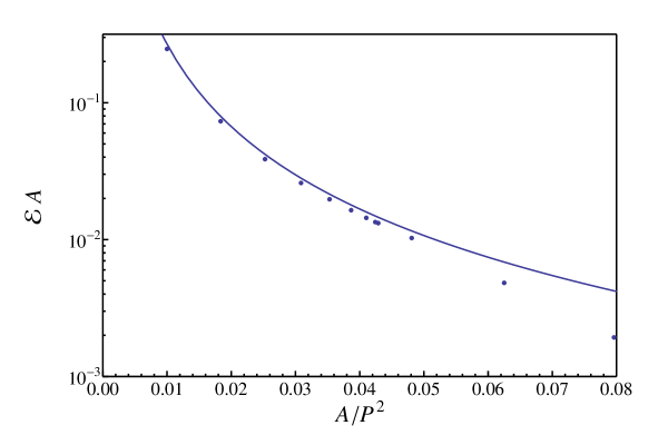
Figure 2: Scalar Casimir energies $\mathcal{E}$ per unit length, scaled by the cross-sectional area $A$, for infinite cylinders having triangular, square, and circular cross sections, obeying Dirichlet boundary conditions on the surfaces. The abscissa is the area $A$ divided by the square of the perimeter $P$ of the cross section. The Weyl volume, surface, and corner divergences have been unambiguously subtracted. Besides the circle and square, the points represent equilateral, right-isosceles, and hemiquilateral triangular cross sections, as well as right triangles calculated numerically. The curve represents the PFA (proximity force approxiation) result.

The Dirichlet energies for tetrahedra, cube [56, 57, 58, 59, 60, 61], and finite (sufficiently short) prisms are negative (attractive). Neumann boundary conditions generally give attractive results as well, as do perfectly conducting electromagnetic boundary conditions for cylinders. These energies are all referring to interior modes of the cavity only, except for spheres and cylinders, where, to exclude curvature divergences, exterior modes are included as well. The new systematics described in [52, 53] go a long way for shedding light on the general behavior of Casimir self-energies, both in sign and magnitude, which have remained elusive for decades.

Because there are no unremovable curvature divergences, Casimir energies may be computed unambiguously in these situations. However, the physical meaning of the results is unclear. Certainly, if one surface is pulled away from a tetrahedral box, it will experience an attractive force due to the closest elements of the surfaces. The self-energy represents the energy required to assemble the complete structure, but it is unclear how such a thing could ever be measured.

4 Magnetic repulsion

Boyer also discovered [6] that a perfectly electrically-conducting plate repels a perfectly magnetically-conductive plate, that is, for one plate, the electric permittivity is taken to infinity, while for the second plate, the magnetic permeability is taken to infinity. Indeed, it is straightforward to show that the Lifshitz energy per area between parallel dielectric and diamagnetic slabs, separated by a vacuum gap of thickness $a$, is

$$\mathcal{E}_{\varepsilon\mu}=\frac{1}{8\pi^{3}}\int_{0}^{\infty}\rmd\zeta\int\rmd^{2}k\bigg{[}\ln\left(1-r_{1}r_{2}^{\prime}\rme^{-2\kappa a}\right)+\ln\left(1-r_{1}^{\prime}r_{2}\rme^{-2\kappa a}\right)\bigg{]},$$ (4.1)

where

$$r_{i}=\frac{\kappa-\kappa_{i}}{\kappa+\kappa_{i}},\quad r_{i}^{\prime}=\frac{\kappa-\kappa^{\prime}_{i}}{\kappa+\kappa^{\prime}_{i}},$$ (4.2)

with

$$\kappa^{2}=k^{2}+\zeta^{2},\quad\kappa^{2}_{1}=k^{2}+\varepsilon\zeta^{2},\quad\kappa_{1}^{\prime}=\kappa_{1}/\varepsilon,\quad\kappa^{2}_{2}=k^{2}+\mu\zeta^{2},\quad\kappa_{2}^{\prime}=\kappa_{2}/\mu.$$ (4.3)

This means in the perfect reflecting limit, $\varepsilon\to\infty$, $\mu\to\infty$,

$$\mathcal{E}_{\rm Boyer}=+\frac{7}{8}\frac{\pi^{2}}{720a^{3}},$$ (4.4)

we get Boyer’s repulsive result [6], $-7/8$ times the Casimir attraction that follows from the appropriate limit of (2.4).

However, materials with such a large magnetic response over a sufficiently large frequency range are difficult to manufacture. One might think that artificial materials, metamaterials, would be a route to magnetic repulsion [62, 63, 64, 65, 66, 67, 68]. Despite some early optimism, the conclusion seems to be settled that repulsion is impossible between metamaterials made from dielectric and metallic components [69, 70, 71]. For recent attempts using dielectric/magnetic setups see [72, 73, 74], who consider nanowires, ferrites, and topological insulators, respectively.

5 Classical repulsion

The discussion in this section is based on [75].

5.1 Repulsion between dipoles

Of course, repulsion occurs in classical situations. Not only do like charges repel, but electric dipoles exhibit regimes in which repulsion occurs as well. Consider the situation illustrated in figure 3.

Figure 3: Configuration of three dipoles, two of which are antiparallel, and one perpendicular to the other two.

Here we have two dipoles, of strength $d_{2}$ and $d_{3}$ lying along the $x$ axis, separated by a distance $a$. A third dipole of strength $d_{1}$ lies along the $z$ axis, a distance $Z$ from the line of the dipoles 2 and 3. If the two parallel dipoles are oppositely directed and of equal strength,

$$\mathbf{d}_{2}=-\mathbf{d}_{3}=d_{2}\mathbf{\hat{x}},$$ (5.1)

and are equally distant from the $z$ axis, and the dipole on the $z$ axis is directed along that axis,

$$\mathbf{d}_{1}=d_{1}\mathbf{\hat{z}},$$ (5.2)

the force on that dipole is along the $z$ axis:

$$F_{z}=3ad_{1}d_{2}\frac{a^{2}/4-4Z^{2}}{(Z^{2}+a^{2}/4)^{7/2}},$$ (5.3)

which changes sign at $Z=a/4$. That is, for distances $Z$ larger than this, the force is attractive (in the $-z$ direction) while for shorter distances the force is repulsive (in the $+z$ direction). Evidently, by symmetry, the dipole-dipole energy vanishes at $z=0$. Consistent with Earnshaw’s theorem [76], the point where the force vanishes is an unstable point with respect to deviations in the $x$ direction.

5.2 Three dimensional aperture interacting with dipole

More interesting is the interaction of a dipole with a conducting screen containing an aperture, for example, a slot or a circular hole. For the case of a dipole, polarized along the symmetry axis, a distance $Z$ directly above a circular aperture of radius $a$ in a conducting plate, the problem can be solved in closed form.

The free three-dimensional Green’s function in cylindrical coordinates has the representation

$$G_{0}(\mathbf{r,r^{\prime}})=\frac{1}{\sqrt{\rho^{2}+(z-z^{\prime})^{2}}}=\int_{0}^{\infty}\rmd k\,J_{0}(k\rho)\rme^{-k|z-z^{\prime}|},$$ (5.4)

from which we can immediately find the Green’s function,

$$G(\mathbf{r,r^{\prime}})=G_{0}(\rho,z-z^{\prime})-G_{0}(\rho,z+z^{\prime}),\quad\rho=\sqrt{(x-x^{\prime})^{2}+(y-y^{\prime})^{2}},$$ (5.5)

so constructed that

$$G(\rho,z=0,z^{\prime})=0.$$ (5.6)

Using this, we can calculate the electrostatic potential at any point above the $z=0$ plane to be

$$\phi(\mathbf{r})=\int_{z>0}(\rmd\mathbf{r^{\prime}})\,G(\mathbf{r,r^{\prime}})\rho(\mathbf{r^{\prime}})+\frac{1}{4\pi}\int_{\rm ap}\rmd S^{\prime}\frac{\partial}{\partial z^{\prime}}G(\mathbf{r,r^{\prime}})\bigg{|}_{z^{\prime}=0}\phi(\mathbf{r^{\prime}}),$$ (5.7)

where the volume integral is over the charge density of the dipole,

$$\rho(\mathbf{r})=-\mathbf{d}\cdot\boldsymbol{\nabla}\delta(\mathbf{r-R}),\quad\mathbf{R}=(0,Z).$$ (5.8)

The surface integral extends only over the aperture because the potential vanishes on the conducting sheet. Using the addition theorem for Bessel functions, we then find for the potential above the plate

$$\phi(\mathbf{r_{\perp}},z>0) = d\left[\frac{z-Z}{[r_{\perp}^{2}+(z-Z)^{2}]^{3/2}}+\frac{z+Z}{[r_{\perp}^{2}+(z+Z)^{2}]^{3/2}}\right]$$ (5.9)

$$\quad\mbox{}+\int_{0}^{\infty}\rmd k\,k\,\rme^{-kz}J_{0}(kr_{\perp})\Phi(k),$$

where the Bessel transform of the potential in the aperture is

$$\Phi(k)=\int_{0}^{\infty}\rmd\rho\,\rho\,J_{0}(k\rho)\phi(\rho,0).$$ (5.10)

Below the aperture there is no contribution from the dipole if we similarly integrate below the $z=0$ plane,

$$\phi(\mathbf{r_{\perp}},z<0)=\int_{0}^{\infty}\rmd k\,k\,\rme^{kz}J_{0}(kr_{\perp})\Phi(k).$$ (5.11)

Then we obtain two integral equations resulting from the continuity of the $z$-component of the electric field in the aperture and the vanishing of the potential on the conductor:

$$d\frac{r_{\perp}^{2}-2Z^{2}}{[r_{\perp}^{2}+Z^{2}]^{5/2}}=\int_{0}^{\infty}\rmd k\,k^{2}J_{0}(kr_{\perp})\Phi(k),\quad r_{\perp}<a,$$ (5.12a)

$$0=\int_{0}^{\infty}\rmd k\,kJ_{0}(kr_{\perp})\Phi(k),\quad r_{\perp}>a.$$ (5.12b)

The solution to these equations is given in Titchmarsh’s book [77], and after a bit of manipulation we obtain

$$\Phi(k)=-\left(\frac{2}{\pi ka}\right)^{1/2}d\int_{0}^{1}\rmd x\,x^{3/2}J_{1/2}(xka)\frac{2Z/a}{(x^{2}+Z^{2}/a^{2})^{2}}.$$ (5.12m)

From this, we can work out the energy of the system from

$$U=-\frac{d}{2}E_{z}(0,Z)=\frac{d}{2}\frac{\partial\phi}{\partial z}\bigg{|}_{z=Z,x=0},$$ (5.12n)

where the factor of 1/2 comes from the fact that this must be the energy required to assemble the system. In computing this energy we must, of course, drop the self-energy of the dipole due to its own field. We encounter the integral

$$\int_{0}^{\infty}\rmd k\,k^{3/2}\rme^{-kZ}J_{1/2}(kax)=2\sqrt{\frac{2xa}{\pi}}\frac{Z}{(x^{2}a^{2}+Z^{2})^{2}},$$ (5.12o)

and then we can express the energy in closed form:

$$U=-\frac{d^{2}}{8Z^{3}}+\frac{d^{2}}{4\pi Z^{3}}\left[\arctan\frac{a}{Z}+\frac{Z}{a}\frac{1+8/3(Z/a)^{2}-(Z/a)^{4}}{(1+Z^{2}/a^{2})^{3}}\right].$$ (5.12p)

This is always negative, but vanishes at infinity and at zero:

$$Z\to 0:\quad U\to-\frac{4}{5\pi}d^{2}\frac{Z^{2}}{a^{5}}.$$ (5.12q)

This means that for some value of $Z\sim a$ the force changes from attractive to repulsive. We find that the force changes sign at $Z=0.742358a$.

The reason why the energy vanishes when the dipole is centered in the aperture is clear: Then the electric field lines are perpendicular to the conducting sheet on the surface, and the sheet could be removed without changing the field configuration.

A similar calculation, with qualitatively identical results, occurs for two conducting half planes separated by an infinite slit [75].

6 Casimir-Polder repulsion between atoms

We now turn to the quantum repulsion. This was first revealed by the numerical results of Levin et al[20], followed by some analytical work [78]. Our group is in the midst of an extensive analysis of Casimir-Polder repulsion. The following discussion first appeared in [79]. The interaction between two polarizable atoms, described by general polarizabilities $\boldsymbol{\alpha}_{1,2}$, with the relative separation vector given by $\mathbf{r}$ is [80, 81]

$$U_{\rm CP}=-\frac{1}{4\pi r^{7}}\left[\frac{13}{2}\Tr\boldsymbol{\alpha}_{1}\cdot\boldsymbol{\alpha}_{2}-28\Tr(\boldsymbol{\alpha}_{1}\cdot\mathbf{\hat{r}})(\boldsymbol{\alpha}_{2}\cdot\mathbf{\hat{r}})+\frac{63}{2}(\mathbf{\hat{r}}\cdot\boldsymbol{\alpha}_{1}\cdot\mathbf{\hat{r}})(\mathbf{\hat{r}}\cdot\boldsymbol{\alpha}_{2}\cdot\mathbf{\hat{r}})\right].$$ (5.12a)

This formula is easily rederived by the multiple scattering technique as explained in [82]. This reduces, in the isotropic case, $\boldsymbol{\alpha}_{i}=\alpha_{i}\boldsymbol{1}$, to the usual Casimir-Polder (CP) energy, $U_{\rm CP}=-\frac{23}{4\pi r^{7}}\alpha_{1}\alpha_{2}$. Suppose the two atoms are only polarizable in perpendicular directions, $\boldsymbol{\alpha}_{1}=\alpha_{1}\mathbf{\hat{z}\hat{z}}$, $\boldsymbol{\alpha}_{2}=\alpha_{2}\mathbf{\hat{x}\hat{x}}$, as shown in figure 4. Choose atom 2 to be at the origin.

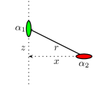
Figure 4: Casimir-Polder interaction between two atoms of polarizability $\boldsymbol{\alpha}_{1}$ and $\boldsymbol{\alpha}_{2}$ separated by a distance $r$. Atom 1 is predominantly polarizable in the $z$ direction, while atom 2 is predominantly polarizable in the $x$ direction. The force on atom 1 in the $z$ direction becomes repulsive sufficiently close to the polarization axis of atom 2 provided both atoms are sufficiently anisotropic.

Then, in terms of the polar angle $\cos\theta=z/r$, the $z$-component of the force on atom 1 is

$$F_{z}=-\frac{63}{8\pi}\frac{\alpha_{1}\alpha_{2}}{x^{8}}\sin^{10}\theta\cos\theta(9-11\sin^{2}\theta).$$ (5.12b)

Here, we are considering motion for fixed $x=r\sin\theta$, in the $y=0$ plane. Evidently, the force is attractive at large distances, vanishing as $\theta\to 0$, but it must change sign at small values of $z$ for fixed $x$, since the energy also vanishes as $\theta\to\pi/2$. The force component in the $z$ direction vanishes when $\sin\theta=3/\sqrt{11}$ or $\theta=1.130$ or 25^∘ from the $x$ axis.

No repulsion occurs if one of the atoms is isotropically polarizable. If both have cylindrically symmetric anisotropies, but with respect to perpendicular axes,

$$\boldsymbol{\alpha}_{1}=(1-\gamma_{1})\alpha_{1}\mathbf{\hat{z}\hat{z}}+\gamma_{1}\alpha_{1}\boldsymbol{1},\quad\boldsymbol{\alpha}_{2}=(1-\gamma_{2})\alpha_{2}\mathbf{\hat{x}\hat{x}}+\gamma_{2}\alpha_{2}\boldsymbol{1},$$ (5.12c)

it is easy to check that, if both are sufficiently anisotropic, repulsion will occur. For example, if $\gamma_{1}=\gamma_{2}$ repulsion in the $z$ direction will take place close to the plane $z=0$ if $\gamma\leq 0.26$.

After [79] was submitted, a paper by Shajesh and Schaden [83] appeared, which rederived these results, and then went on to extend the calculation to Casimir-Polder repulsion by an anisotropic dilute dielectric sheet with a circular aperture. The authors quite correctly point out that the statement in [75] that no repulsion is possible in the weak-coupling regime is erroneous. That inference was based on isotropic media; anisotropy is necessary for repulsion.

Here we extend the calculations of [83]. We consider an anisotropic polarizable atom directly above a tenuous anisotropic slab containing a circular aperture, as shown in figure 5.

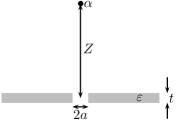
Figure 5: Three-dimensional geometry of a polarizable atom a distance $Z$ above a dielectric slab of thickness $t$ with a circular aperture of radius $a$.

Here we assume that the atom is only polarizable in the $z$ direction,

$$\boldsymbol{\alpha}_{1}=\alpha_{1}\mathbf{\hat{z}\hat{z}},$$ (5.12d)

while the slab is composed of atoms only transversely polarizable,

$$\boldsymbol{\alpha}_{2}=\alpha_{2}(\mathbf{\hat{x}\hat{x}+\hat{y}\hat{y}}).$$ (5.12e)

Starting from (5.12a), we use cylindrical coordinates with origin at the center of the aperture, and find the interaction energy between atom 1 at $(0,0,Z)$, and atom 2 at $(\rho,0,z)$ to be

$$U_{\rm CP}=-\frac{63\alpha_{1}\alpha_{2}}{8\pi r^{7}}\left(\frac{Z-z}{r}\right)^{2}\left(\frac{\rho}{r}\right)^{2},$$ (5.12f)

which when integrated over the slab made up of the type-2 atoms gives the quantum interaction energy

$$E = -\frac{63\alpha_{1}\alpha_{2}n_{2}}{8\pi}\int_{a}^{\infty}\rmd\rho\,\rho\int_{0}^{2\pi}\rmd\theta\int_{-t/2}^{t/2}\rmd z\frac{(Z-z)^{2}\rho^{2}}{\left[(Z-z)^{2}+\rho^{2}\right]^{11/2}}$$ (5.12g)

$$= -\frac{63\alpha_{1}\alpha_{2}n_{2}}{2a^{4}}\left[e(Z/a+t/2a)-e(Z/a-t/2a)\right],$$

where $n_{2}$ is the number density of atoms in the slab, $t$ is the thickness of the slab, and the atom is located a distance $Z$ directly above the aperture. Here we have defined the function

$$e(x)=\frac{x^{3}}{5}\frac{15+14x^{2}+4x^{4}}{(1+x^{2})^{7/2}}.$$ (5.12h)

Such an atom sufficiently close to the aperture experiences a repulsive force. Define a dimensionless parameter $\delta$ that measures the height of the atom above the top of the aperture,

$$Z=\frac{t}{2}+a\delta.$$ (5.12i)

For a thick aperture, $t/a\gg 1$, it is easy to check that that the force changes sign very close to the opening of the aperture,

$$\delta=\frac{\sqrt{2}}{3}\left(\frac{t}{a}\right)^{-5/2};$$ (5.12j)

for example, when $t/a=10$, $\delta=1.5\times 10^{-3}$. When the aperture is very thin, $t/a\ll 1$, the value of $\delta$ for which repulsion sets in becomes independent of $t/a$, $\delta=0.5566$, which again agrees with the result of [83].

7 Casimir-Polder force between an atom and a conducting wedge

7.1 General formula for Casimir-Polder interaction

Now we turn to the CP interaction between an atom and a dielectric or conducting body. Our starting point is the general expression for the vacuum energy [82]

$$U=\frac{i}{2}\Tr\ln{\boldsymbol{\Gamma}\boldsymbol{\Gamma}}_{0}^{-1},$$ (5.12a)

where $\boldsymbol{\Gamma}$ is the full Green’s dyadic for the problem, and $\boldsymbol{\Gamma}_{0}^{-1}$ is the inverse of the free Green’s dyadic, namely

$$\boldsymbol{\Gamma}_{0}^{-1}=\frac{1}{\omega^{2}}\boldsymbol{\nabla}\times\boldsymbol{\nabla}\times-\boldsymbol{1}.$$ (5.12b)

In the presence of a potential $\mathbf{V}$, the full Green’s dyadic has the symbolic form

$$\boldsymbol{\Gamma}=(\boldsymbol{1}-\boldsymbol{\Gamma}_{0}\mathbf{V})^{-1}\boldsymbol{\Gamma}_{0}.$$ (5.12c)

Here we are thinking of the interaction between a dielectric medium, characterized by an isotropic permittivity, so $V_{1}=\varepsilon-1$, and a polarizable atom, represented by a polarizability dyadic, as shown in figure 5,

$$\mathbf{V}_{2}=4\pi\boldsymbol{\alpha}\delta(\mathbf{r-R}),$$ (5.12d)

where $\mathbf{R}$ is the position of the dipole. We are only interested in a single interaction with the latter potential, so we have for the interaction energy

$$U_{12}=\Tr\mathbf{V}_{2}\frac{\delta}{\delta V_{1}}\left[-\frac{i}{2}\ln\left(1-\boldsymbol{\Gamma}_{0}V_{1}\right)\right]=\frac{i}{2}\Tr\left(\boldsymbol{\Gamma}_{1}-\boldsymbol{\Gamma}_{0}\right)\mathbf{V}_{2},$$ (5.12e)

where we have used (5.12c) for the potential $V_{1}$ describing the dielectric slab plus aperture and we have subtracted the term that represents the self-energy of the atom with its own field. This subtraction happens automatically if we start from the “$TGTG$” form,

$$U_{12}=-\frac{i}{2}\Tr\ln\left(\boldsymbol{1}-\boldsymbol{\Gamma}_{1}\mathbf{V}_{1}\boldsymbol{\Gamma}_{2}\mathbf{V}_{2}\right)\approx\frac{i}{2}\Tr\boldsymbol{\Gamma}_{1}\mathbf{V}_{1}\boldsymbol{\Gamma}_{0}\mathbf{V}_{2}=\frac{i}{2}\Tr\left(\boldsymbol{\Gamma}_{1}-\boldsymbol{\Gamma}_{0}\right)\mathbf{V}_{2},$$ (5.12f)

because $\mathbf{V}_{2}$ is weak. This implies the Casimir-Polder expression for the interaction between the polarizable atom and the dielectric

$$U_{\rm CP}=-\int_{-\infty}^{\infty}\rmd\zeta\tr\boldsymbol{\alpha}\cdot(\boldsymbol{\Gamma}-\boldsymbol{\Gamma}_{0})(Z,Z).$$ (5.12g)

(Note that although we use Gaussian units otherwise, the Green’s dyadics are still expressed in terms of Heaviside-Lorentz units; otherwise, factors of $4\pi$ appear.)

7.2 Wedge calculation

The interaction between a polarizable atom and a perfectly conducting half-plane is a special case of the vacuum interaction between such an atom and a conducting wedge. For the case of an isotropic atom, this was considered by Brevik, Lygren, and Marachevsky [84]. (This followed on earlier work by Brevik and Lygren [85] and DeRaad and Milton [54].) In terms of the opening dihedral angle of the wedge $\Omega$, which we describe in terms of the variable $p=\pi/\Omega$, the electromagnetic Green’s dyadic has the form (here the translational direction is denoted by $y$, and one plane of the wedge lies in the $z=0$ plane, the other intersecting the $xz$ plane on the line $\theta=\Omega$—see figure 6)

$$\boldsymbol{\Gamma}(\mathbf{r,r^{\prime}})=2p\sum_{m=0}^{\infty}{}^{\prime}\int\frac{\rmd k}{2\pi}\bigg{[}-\boldsymbol{\mathcal{M}}\boldsymbol{\mathcal{M}}^{\prime*}(\nabla_{\perp}^{2}-k^{2})\frac{1}{\omega^{2}}F_{mp}(\rho,\rho^{\prime})\frac{\cos mp\theta\cos mp\theta^{\prime}}{\pi}\rme^{\rmi k(y-y^{\prime})}$$

$$\mbox{}+\boldsymbol{\mathcal{N}}\boldsymbol{\mathcal{N}}^{\prime*}\frac{1}{\omega}G_{mp}(\rho,\rho^{\prime})\frac{\sin mp\theta\sin mp\theta^{\prime}}{\pi}\rme^{\rmi k(y-y^{\prime})}\bigg{]}.$$ (5.12h)

The first term here refers to TE (H) modes, the second to TM (E) modes. The prime on the summation sign means that the $m=0$ term is counted with half weight. In the polar coordinates in the $xz$ plane, $\rho$ and $\theta$, the H and E mode operators are

$$\boldsymbol{\mathcal{M}}=\boldsymbol{\hat{\rho}}\frac{\partial}{\rho\partial\theta}-\boldsymbol{\hat{\theta}}\frac{\partial}{\partial\rho},$$ (5.12ia)

$$\boldsymbol{\mathcal{N}}=\rmi k\left(\boldsymbol{\hat{\rho}}\frac{\partial}{\partial\rho}+\boldsymbol{\hat{\theta}}\frac{\partial}{\rho\partial\theta}\right)-\mathbf{\hat{y}}\nabla_{\perp}^{2},$$ (5.12ib)

where the transverse Laplacian is

$$\nabla_{\perp}^{2}=\frac{1}{\rho}\frac{\partial}{\partial\rho}\rho\frac{\partial}{\partial\rho}+\frac{1}{\rho^{2}}\frac{\partial^{2}}{\partial\theta^{2}}.$$ (5.12ij)

In this situation, the boundaries are entirely in planes of constant $\theta$, so the radial Green’s functions are equal to the free Green’s function

$$\frac{1}{\omega^{2}}F_{mp}(\rho,\rho^{\prime})=\frac{1}{\omega}G_{mp}(\rho,\rho^{\prime})=-\frac{\rmi\pi}{2\lambda^{2}}J_{mp}(\lambda\rho_{<})H^{(1)}_{mp}(\lambda\rho_{>}),$$ (5.12ik)

with $\lambda^{2}=\omega^{2}-k^{2}$. We will immediately make the Euclidean rotation, $\omega\to\rmi\zeta$, where $\lambda\to\rmi\kappa$, $\kappa^{2}=\zeta^{2}+k^{2}$, so the free Green’s functions become $-\kappa^{-2}I_{mp}(\kappa\rho_{<})K_{mp}(\kappa\rho_{>})$.

Figure 6: Polarizable atom, located at polar coordinates $\rho$, $\theta$, within a conducting wedge with dihedral angle $\Omega$.

We start by considering the most favorable case for CP repulsion, where the atom is only polarizable in the $z$ direction, that is, only $\alpha_{zz}\neq 0$. In the static limit, the only component of the Green’s dyadic that contributes is

$$\int\frac{\rmd\zeta}{2\pi}\Gamma_{zz}=\frac{2p}{4\pi^{3}}\int\rmd k\,\rmd\zeta\bigg{\{}\left[\zeta^{2}\sin^{2}\theta\sin^{2}mp\theta-k^{2}\cos^{2}\theta\cos^{2}mp\theta\right]$$

$$\quad\times\frac{m^{2}p^{2}}{\kappa^{2}\rho_{<}\rho_{>}}I_{mp}(\kappa\rho_{<})K_{mp}(\kappa\rho_{>})$$

$$\quad\mbox{}-\left[k^{2}\sin^{2}\theta\sin^{2}mp\theta-\zeta^{2}\cos^{2}\theta\cos^{2}mp\theta\right]I^{\prime}_{mp}(\kappa\rho_{<})K^{\prime}_{mp}(\kappa\rho_{>})\bigg{\}}.$$ (5.12il)

Here we note that the off diagonal $\rho$-$\theta$ terms in $\boldsymbol{\Gamma}$ cancel. We have regulated the result by point-splitting in the radial coordinate. At the end of the calculation, the limit $\rho_{<}\to\rho_{>}=\rho$ is to be taken.

Now the integral over the Bessel functions is given by

$$\int_{0}^{\infty}\rmd\kappa\,\kappa\,I_{\nu}(\kappa\rho_{<})K_{\nu}(\kappa\rho_{>})=\frac{\xi^{\nu}}{\rho_{>}^{2}(1-\xi^{2})},$$ (5.12im)

where $\xi=\rho_{<}/\rho_{>}$. After that the $m$ sum is easily carried out by summing a geometrical series. Care must also be taken with the $m=0$ term in the cosine series. The result of a straightforward calculation leads to

$$\int\frac{\rmd\zeta}{2\pi}\Gamma_{zz}=-\frac{\cos 2\theta}{\pi^{2}\rho^{4}}\frac{1}{(\xi-1)^{4}}+\mbox{finite},$$ (5.12in)

where the term divergent as $\xi\to 1$ may, through a similar calculation, be shown to be that corresponding to the vacuum in absence of the wedge, that is, that obtained from the free Green’s dyadic. Therefore, we must subtract this term off, to obtain the static Casimir energy (5.12g), which for this situation is

$$U^{zz}_{\rm CP}=-\frac{\alpha_{zz}(0)}{8\pi}\frac{1}{\rho^{4}\sin^{4}p\theta}\left[p^{4}-\frac{2}{3}p^{2}(p^{2}-1)\sin^{2}p\theta+\frac{(p^{2}-1)(p^{2}+11)}{45}\sin^{4}p\theta\cos 2\theta\right].$$

(5.12io)

This result can also be derived from the closed form for the Green’s function given by Lukosz [58].

A small check of this result is that as $\theta\to 0$ (or $\theta\to\Omega$) we recover the expected Casimir-Polder result for an atom above an infinite plane:

$$U_{\rm CP}^{zz}\to-\frac{\alpha_{zz}(0)}{8\pi Z^{4}},$$ (5.12ip)

in terms of the distance of the atom above the plane, $Z=\rho\theta$. This limit is also obtained when $p\to 1$, for when $\Omega=\pi$ we are describing a perfectly conducting infinite plane.

A very similar calculation gives the result for an isotropic atom, $\boldsymbol{\alpha}=\alpha\boldsymbol{1}$, which was first given in [84]:

$$U_{\rm CP}=-\frac{3\alpha(0)}{8\pi\rho^{4}\sin^{4}p\theta}\left[p^{4}-\frac{2}{3}p^{2}(p^{2}-1)\sin^{2}p\theta-\frac{1}{3}\frac{1}{45}(p^{2}-1)(p^{2}+11)\sin^{4}p\theta\right].$$ (5.12iq)

Note that this is not three times $U_{\rm CP}^{zz}$ in (5.12io) because the $\cos 2\theta$ factor in the last term in the latter is replaced by $-1/3$ here. This case was reconsidered recently, for example, in [86].

Figure 7: Polarizable atom, above a half conducting plane, free to move on a line perpendicular to the plane but a distance $X$ to the left of the plane.

7.3 Repulsion by a conducting half-plane

Let us consider the special case $p=1/2$, that is $\Omega=2\pi$, the case of a semi-infinite conducting plane. This was the situation considered, for anisotropic atoms, in recent papers by Eberlein and Zietal [87, 88]. Note that in such a case, for the completely anisotropic atom, $U_{\rm CP}^{zz}=0$ at $\theta=\pi$, which is obvious by symmetry.

Consider a particle free to move along a line parallel to the $z$ axis, a distance $X$ to the left of the semi-infinite plane. See figure 7. The half-plane $z=0$, $x<0$ constitutes an aperture of infinite width. With $X$ fixed, we can describe the trajectory by $u=X/\rho=-\cos\theta$, which ranges from zero to one. The polar angle is given by

$$\sin^{2}\frac{\theta}{2}=\frac{1+u}{2}.$$ (5.12ir)

The energy for an isotropic atom is given by

$$U_{\rm CP}=-\frac{\alpha(0)}{32\pi}\frac{1}{X^{4}}V(u),$$ (5.12is)

where

$$V(u)=3u^{4}\left[\frac{1}{(1+u)^{2}}+\frac{1}{u+1}+\frac{1}{4}\right].$$ (5.12it)

The energy for the completely anisotropic atom is

$$V_{zz}=\frac{1}{3}V(u)+\frac{u^{4}}{2}(1-3u^{2}).$$ (5.12iu)

Let us consider instead a cylindrically symmetric polarizable atom in which

$$\boldsymbol{\alpha}=\alpha_{zz}\mathbf{\hat{z}\hat{z}}+\gamma\alpha_{zz}(\mathbf{\hat{x}\hat{x}+\hat{y}\hat{y}})=\alpha_{zz}(1-\gamma)\mathbf{\hat{z}\hat{z}}+\gamma\alpha_{zz}\boldsymbol{1},$$ (5.12iv)

where $\gamma$ is the ratio of the transverse polarizability to the longitudinal polarizability of the atom. Then the effective potential is

$$(1-\gamma)V_{zz}+\gamma V,$$ (5.12iw)

and the $z$-component of the force on the atom is

$$F^{\gamma}_{z}=-\frac{\alpha_{zz}(0)}{32\pi}\frac{1}{X^{5}}u^{2}\sqrt{1-u^{2}}\frac{\rmd}{\rmd u}\left[\frac{1}{2}u^{4}(1-\gamma)(1-3u^{2})+\frac{1}{3}(1+2\gamma)V(u)\right],$$ (5.12ix)

where $V$ is given by (5.12it). Note that the energy (5.12iw), or the quantity in square brackets in (5.12ix), only vanishes at $u=1$ ($\theta=\pi$, the plane of the conductor) when $\gamma=0$. Thus, the symmetry argument given in [20] applies only for the completely anisotropic case. The force is plotted in figures 8, 9. It will be seen that if $\gamma$ is sufficiently small, when the atom is sufficiently close to the plane of the plate the $z$-component of the force is repulsive rather than attractive. The critical value of $\gamma$ is $\gamma_{c}=1/4$. This is a completely analytic exact analog of the numerical calculations shown in [20], where the interaction was considered between a conducting plane with an aperture (circular hole or slit), and a conducting cylindrical or ellipsoidal object. Our calculation demonstrates that three-body effects are not required to exhibit Casimir-Polder repulsion. In fact, three-body effects are rather small [78].

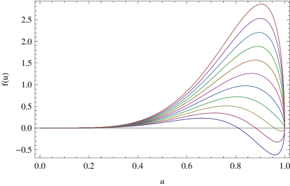
Figure 8: The $z$-component of the force between an anisotropic atom (with ratio of transverse to longitudinal polarizabilities $\gamma$) and a semi-infinite perfectly conducting plane, $z=0$, $x>0$. $F_{z}=-\alpha_{zz}f(u)/(32\pi X^{5})$ in terms of the variable $u=X/\rho=-\cos\theta$. The atom lies on the line $y=0$, $x=-X$, and $\rho$ is the distance from the edge of the plane to the atom. Here, $f>0$ corresponds to an attractive force on the $z$ direction, and $f<0$ corresponds to a repulsive force. The different curves correspond to different values of $\gamma$, $\gamma=0$ to 1 by steps of 0.1, from bottom to top. For $\gamma<1/4$ a repulsive regime always occurs when the atom is sufficiently close to the plane of the conductor.

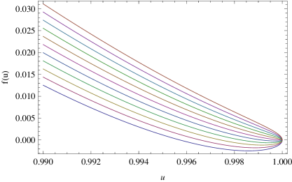
Figure 9: Same as figure 8. The region close to the plane, $1\geq u\geq 0.99$, with $\gamma$ near the critical value of 1/4. Here from bottom to top are shown the results for values of $\gamma$ from 0.245 to 0.255 by steps of 0.001.

It is interesting to observe that the same critical value of $\gamma$ occurs in the nonretarded regime for a circular aperture, as follows from a simple computation based on the result of [89]. For example, applying the result there for an atom with polarizability given by (5.12iv) placed a distance $Z$ along the symmetry axis of a circular aperture of radius $a$ in a conducting plane gives an energy

$$U=-\frac{1}{16\pi^{2}}\int_{-\infty}^{\infty}\rmd\zeta\,\alpha_{zz}(\zeta)\frac{1}{Z^{3}}\Bigg{\{}(1+\gamma)\left(\frac{\pi}{2}+\arctan\frac{Z^{2}-a^{2}}{2aZ}\right)$$

$$\mbox{}+\frac{2aZ}{(Z^{2}+a^{2})^{3}}\left[(1+\gamma)(Z^{4}-a^{4})-\frac{8}{3}(1-\gamma)a^{2}Z^{2}\right]\Bigg{\}}.$$ (5.12iy)

It is easy to see that this has a minimum for $z>0$, and hence there is a repulsive force close to the aperture, provided $\gamma<\gamma_{c}=1/4$.

7.4 Repulsion by a wedge

It is very easy to generalize the above result for a wedge, $p>1/2$. That is, we want to consider a strongly anisotropic atom, with only $\alpha_{zz}$ significant, to the left of a wedge of opening angle

$$\beta=2\pi-\Omega,$$ (5.12iz)

as shown in figure 10.

Figure 10: A polarizable atom outside a perfectly conducting wedge of interior angle $\beta$. The atom is located at polar angles $\rho$, $\phi$ relative to the symmetry plane of the wedge.

We want the $z$ axis to be perpendicular to the symmetry plane of the wedge so the relation between the polar angle of the atom and the angle to the symmetry line is

$$\phi=\theta+\beta/2,$$ (5.12iaa)

where, as before, $\theta$ is the angle relative to the top surface of the wedge. Then, it is obvious that the formula for the Casimir-Polder energy (5.12io) is changed only by the replacement of $\cos 2\theta$ by $\cos 2\phi$, with no change in $\sin p\theta$. Now we can ask how the region of repulsion depends on the wedge angle $\beta$.

Write for an atom on the line $x=-X$

$$U^{zz}_{\rm CP}=-\frac{\alpha_{zz}(0)}{8\pi X^{4}}V(\phi),$$ (5.12iab)

where

$$V(\phi)=\cos^{4}\phi\left[\frac{p^{4}}{\sin^{4}\frac{\pi}{2}\frac{\phi-\beta/2}{\pi-\beta/2}}-\frac{2}{3}\frac{p^{2}(p^{2}-1)}{\sin^{2}\frac{\pi}{2}\frac{\phi-\beta/2}{\pi-\beta/2}}+\frac{1}{45}(p^{2}-1)(p^{2}+11)\cos 2\phi\right].$$ (5.12iac)

At the point of closest approach,

$$V(\pi)=\frac{1}{45}(4p^{2}-1)(4p^{2}+11),$$ (5.12iad)

so the potential vanishes at that point only for the half-plane case, $p=1/2$, as noted above. The force in the $z$ direction is

$$F_{z}=-\frac{\alpha_{zz}}{8\pi}\frac{1}{X^{5}}f(\phi),$$ (5.12iaea)

$$f(\phi)=\cos^{2}\phi\frac{\partial V(\phi)}{\partial\phi}.$$ (5.12iaeb)

Figure 11 shows the force as a function of $\phi$ for fixed $X$. It will be seen that the force has a repulsive region for angles close enough to the apex of the wedge, provided that the wedge angle is not too large. The critical wedge angle is actually rather large, $\beta_{c}=1.87795$, or about 108^∘. For larger angles, the $z$-component of the force exhibits only attraction. Of course, the force is zero for $\beta=\pi$ ($p=1$) because then the geometry is translationally invariant in the $z$ direction.

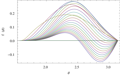
Figure 11: The $z$-component of the force on an completely anisotropic atom moving on a line perpendicular to a wedge. The different curves are for various values of $\beta$ from 0 to $\pi$ by steps of $\pi/20$, from bottom up. The last few values of $\beta$ have a markedly different character from the others.

8 Repulsion of an atom by a conducting cylinder

In this section, we consider the interaction of an anisotropic atom with a perfectly conducting, infinitely long, cylindrical shell. As above, we start from (5.12g), and assume that the polarizability of the atom has negligible frequency dependence (static approximation), and, in order to maximize the repulsive effect, the atom is only polarizable in the $z$ direction, the direction of the trajectory (assumed not to intersect the cylinder). Thus, the quantity we need to compute for a conducting cylinder of radius $a$ is given by [90]

$$\int_{-\infty}^{\infty}\frac{\rmd\zeta}{2\pi}\Gamma_{zz}(r,\theta)=\sum_{m=-\infty}^{\infty}\int_{0}^{\infty}\frac{\rmd\kappa}{(2\pi)^{3}}\frac{\pi}{2a}\frac{1}{K_{m}(\kappa a)K^{\prime}_{m}(\kappa a)}\bigg{\{}\frac{m^{2}}{r^{2}}K_{m}^{2}(\kappa r)+\kappa^{2}K_{m}^{\prime 2}(\kappa r)$$

$$\quad\mbox{}-\cos 2\theta\kappa a[I_{m}(\kappa a)K_{m}(\kappa a)]^{\prime}\left(-\frac{m^{2}}{r^{2}}K_{m}^{2}(\kappa r)+\kappa^{2}K_{m}^{\prime 2}(\kappa r)\right)\bigg{\}}.$$ (5.12iaea)

The geometry we are considering is illustrated in figure 12.

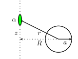
Figure 12: Interaction between an anisotropically polarizable atom and a conducting cylinder of radius $a$. The force on the atom along a line which does not intersect the cylinder is considered. If the atom is only polarizable in that direction, and the line lies sufficiently far from the cylinder, the force component along the line changes sign near the point of closest approach.

It gives greater insight to give the transverse electric (TE) and transverse magnetic (TM) contributions to the CP energy:

$$E^{\rm TE}_{\rm CP}=-\frac{\alpha_{zz}}{4\pi}\sum_{m=-\infty}^{\infty}\int_{0}^{\infty}d\kappa\,\kappa\frac{I^{\prime}_{m}(\kappa a)}{K^{\prime}_{m}(\kappa a)}\left[\frac{\cos^{2}\theta}{r^{2}}m^{2}K_{m}^{2}(\kappa r)+\kappa^{2}\sin^{2}\theta K_{m}^{\prime 2}(\kappa r)\right],$$ (5.12iaeba)

$$E^{\rm TM}_{\rm CP}=\frac{\alpha_{zz}}{4\pi}\sum_{m=-\infty}^{\infty}\int_{0}^{\infty}d\kappa\,\kappa\frac{I_{m}(\kappa a)}{K_{m}(\kappa a)}\left[\frac{\sin^{2}\theta}{r^{2}}m^{2}K_{m}^{2}(\kappa r)+\kappa^{2}\cos^{2}\theta K_{m}^{\prime 2}(\kappa r)\right].$$ (5.12iaebb)

The distance of the atom from the center of the cylinder is $r=R/\sin\theta$, where $R$ is the distance of closest approach and $\theta$ is the polar angle, which ranges from 0 when the atom is at infinity to $\pi/2$ when the atom is closest to the cylinder.

At large distances, the CP force is dominated by the $m=0$ term in the energy sum. Figure 13 shows that for $m=0$ the TM mode dominates except near the position of closest approach, where only the TE mode is nonzero. This indicates that there is a region of repulsion near $\theta=\pi/2$, since the total energy has a minimum for small $\psi=\pi/2-\theta$. This effect is partially washed out by including higher $m$ modes, as seen in figure 14, which shows the effect of including the first 5 $m$ values. But the repulsion goes away if the line of motion passes too close to the cylinder. Numerically, we have found that to have repulsion close to the plane of closest approach requires that $a/R<0.15$.

What about the analagous calculation of the CP force between a polarizable atom and a conducting sphere? Because the latter is symmetric, it is obvious that there can be no repulsion at large distances, because then this is the CP interaction between one anisotropic atom and an isotropic one. In fact, numerical calculation reveals that there is no repulsive regime for even a completely anisotropic atom and a conducting sphere at any separation distance, as discussed in more detail in [79].

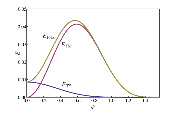
Figure 13: $m=0$ contributions to the Casimir-Polder energy between an anisotropic atom and a conducting cylinder. The (generally) lowest curve (blue) is the TE contribution, the second (magenta) is the TM contribution, and the top curve (yellow) is the total CP energy. In this case, the distance of closest approach of the atom is taken to be 10 times the radius of the cylinder. The energy $E$ is plotted as a function of $\psi=\pi/2-\theta$.

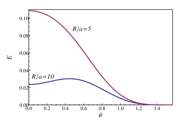
Figure 14: The CP energy between an anisotropic atom and a conducting cylinder. Plotted is the total CP energy, the upper curve for the distance of closest approach $R$ being 5 times the cylinder radius $a$, the lower curve for the distance of closest approach 10 times the radius. The curves move up slightly as more $m$ terms are included, but have completely converged by the time $m=3$ is included. Repulsion is clearly observed when $R/a=10$, but not for $R/a=5$.

9 Conclusions and outlook

We have surveyed some of the older and recent work on situations in which both classical and quantum repulsion between polarizable objects can occur, with particular stress on the analytic work carried out by our group. This is a subject of great current interest, with many new results emerging, so this brief overview can hardly be definitive. Especially interesting would be experimental verification of some of these effects; one might suppose that Rydberg atoms in a high $l$ state would be sufficiently anisotropic to experience repulsion by a suitably structured substrate. However, this now seems unlikely, since it is very difficult to achieve an anisotropy greater than 1/3. A Rydberg atom may be very oblong, but its chief transitions are to more isotropic states. This will be discussed in more detail in a forthcoming paper.

References

References

- [1] Dzyaloshinskii I D, Lifshitz E M and Pitaevskii L P 1961 Usp. Fiz. Nauk 73 381 [Engl. transl.: Sov. Phys. Usp. 4 153; Adv. Phys. 10 165 ]
- [2] Sabisky E S and Anderson C H 1973 Phys. Rev. A 7 790
- [3] Munday J, Capasso F and Parsegian V A 2009 Nature 457 170
- [4] Boyer T H 1968 Phys. Rev. 174 1764
- [5] Casimir H B G 1953 Physica 19 846
- [6] Boyer T H 1974 Phys. Rev. A 9 2078
- [7] Pendry J B 2000 Phys. Rev. Lett. 85 3966
- [8] Leonhardt U and Philbin T G 2007 New J. Phys. 9 254
- [9] Sambale A, Welsch D-G, Dung H T and Buhmann S Y 2008 Phys. Rev. A 78 053828
- [10] Sambale A, Buhmann S Y, Dung H T and Welsch D-G 2009 Phys. Scripta T135 014019
- [11] Barton G 1970 Proc. R. Soc. London A 320 251
- [12] Ellingsen S Å, Buhmann S Y and Scheel S 2009 Phys. Rev. A 79 052903
- [13] Crosse J A, Ellingsen S Å, Clements K, Buhmann S Y and Scheel S 2010 Phys. Rev. A 82 010901(R)
- [14] Ellingsen S Å, Buhmann S Y and Scheel S 2009 Phys. Rev. A 80 022901
- [15] Ellingsen S Å, Buhmann S Y and Scheel S 2010 Phys. Rev. A 82 032516
- [16] Sambale A, Buhmann S Y, Dung H T and Welsch D-G 2009 Phys. Rev. A 80 051801(R)
- [17] Antezza M, Pitaevskii L P and Stringari S 2005 Phys. Rev. Lett. 95 113202
- [18] Antezza M, Pitaevskii L P, Stringari S and Svetovoy V B 2008 Phys. Rev. A 77 022901
- [19] Golyk V A, Krüger M, Homer Reid M T, and Kardar M 2012 Phys. Rev. D 85 065011
- [20] Levin M, McCauley A P, Rodriguez A W, Homer Reid M T and Johnson S G 2010 Phys. Rev. Lett. 105 090403
- [21] Schwinger J, DeRaad, Jr., L L and Milton K 1978 Ann. Phys. (NY) 115 1
- [22] Milton K A 2001 The Casimir Effect (Singapore: World Scientific)
- [23] Bordag M, Klimchitskaya G L, Mohideen U and Mostepanenko V M 2009 Advances in the Casimir Effect (Oxford: Oxford University Press)
- [24] Milton K A 2004 J. Phys. A 37 R209
- [25] Lambrecht A, Maia Neto P A and Reynaud S (2006) New J. Phys 8 243
- [26] Milton K A, Wagner J, Parashar P and Brevik I 2010 Phys. Rev. D 81 065007
- [27] Bordag M 2012 Phys. Rev. D 85 025005
- [28] Milling A, Mulvaney P and Larson I 1996 J. Colloid Interf. Sci. 180 460
- [29] Meurk A, Luckham P F and Bergstrom L 1997 Langmuir 13 3896
- [30] Lee S and Sigmund W M 2001 J. Colloid Interf. Sci. 243 365
- [31] Lee S and Sigmund W M 2002 J. Colloids Surf. A 204 43
- [32] Feiler A A, Bergström L and Rutland M W 2008 Langmuir 24 2274
- [33] Anderson C H and Sabisky E S 1972 Phys. Rev. Lett. 1972 28 80
- [34] Richmond P and Ninham B W 1971 J. Low Temp. Phys. 5 177
- [35] Richmond P and Ninham B W 1971 Solid State Commun. 9 1045
- [36] Hauxwell F and Ottewill R H 1970 J. Colloid Interf. Sci. 34 473
- [37] Ninham B W and Parsegian V A 1970 Biophys. J. 10 647
- [38] Elbaum M and Schick M 1991 Phys. Rev. Lett. 66 1713
- [39] Boström M, Sernelius B E, Brevik I and Ninham B W 2012 Phys. Rev. A 85 010701
- [40] Boström M and Sernelius B E 2012 Phys. Rev. A 85 012508
- [41] Davies B 1972 J. Math. Phys. 13 1324
- [42] Balian R and Duplantier B 1978 Ann. Phys. 112 165
- [43] Milton K A, DeRaad, Jr., L L and Schwinger J 1978 Ann. Phys. (NY) 115 388
- [44] Bender C M and Milton K A 1994 Phys. Rev. D 50 6547
- [45] Leseduarte S and Romeo A 1996 Europhys. Lett. 34 79
- [46] Leseduarte S and Romeo A 1996 Ann. Phys. (NY) 250 448
- [47] Leseduarte S and Romeo A 1996 Comm. Math. Phys. 193 317
- [48] Milton K A 1997 Phys. Rev. D 55 4940
- [49] Kolomeisky E B, Zaidi H, Langsjoen L and Straley J P 2011 arXiv:1110.0421
- [50] Fulling S A, private communication
- [51] Milton K A 2012 paper in preparation
- [52] Abalo E K, Milton K A and Kaplan L 2010 Phys. Rev. D 82 125007
- [53] Abalo E K, Milton K A and Kaplan L 2012 Phys. Rev. D, submitted, arXiv:1202.0908
- [54] DeRaad, Jr., L L and Milton K A 1981 Ann. Phys. (NY) 136 229
- [55] Gosdzinsky P and Romeo A 1998 Phys. Lett. B 441 265
- [56] Lukosz W 1971 Physica 56 109
- [57] Lukosz W 1973 Z. Phys. 258 99
- [58] Lukosz W 1973 Z. Phys. 262 327
- [59] Ambjørn J and Wolfram S 1983 Ann. Phys. (NY) 147 1
- [60] Ruggiero J R, Zimerman A H and Villani A 1977 Rev. Bras. Fiz. 7 663
- [61] Ruggiero J R, Zimerman A H and Villani A 1980 J. Phys. A 13 361
- [62] Henkel C and Joulain K 2005 Europhys. Lett. 72 929
- [63] Pirozhenko I G and Lambrecht A 2008 J. Phys. A 41 164015
- [64] Rosa F S S, Dalvit D A R, and Milonni P W 2008 Phys. Rev. Lett. 100 183602
- [65] Rosa F S S, Dalvit D A R, and Milonni P W 2008 Phys. Rev. A 78 032117
- [66] Zhao R, Zhou J, Koschny Th, Economou E N and Soukoulis C M 2009 Phys. Rev. Lett. 103 103602
- [67] M. G. Silveirinha M G and S. I. Maslovski S I 2010 Phys. Rev. Lett. 105 189301
- [68] Zhao R, Zhou J, Koschny Th, Economou E N and Soukoulis C M 2010 Phys. Rev. Lett. 105 189302
- [69] Yannopapas V and Vitanov N V 2009 Phys. Rev. Lett. 103, 120401
- [70] Silveirinha M G and Maslovski S I 2010 Phys. Rev. A 82 052508
- [71] McCauley A P et al2010 Phys. Rev. B 82 165108
- [72] Maslovski S I and Silveirinha M G 2011 Phys. Rev. A 83 022508
- [73] Zeng R and Yang Y 2011 Phys. Rev. A 83 012517
- [74] Grushin A G and Cortijo A 2011 Phys. Rev. Lett. 106 020403
- [75] Milton K A, Abalo E K, Parashar P, Pourtolami N, Brevik I and Ellingsen S. Å 2011 Phys. Rev. A 83 062507
- [76] Stratton J A 1941 Electromagnetic Theory (New York: McGraw-Hill)
- [77] Titchmarsh E C 1948 Theory of Fourier Integrals (Oxford: Oxford University Press)
- [78] Maghrebi M F 2011 Phys. Rev. D 83 045004
- [79] Milton K A, Parashar P, Pourtolami N, and Brevik I 2012 Phys. Rev. D 85 025008
- [80] Craig D P and Power E A 1969 Chem. Phys. Lett. 3, 195
- [81] Craig D P and Power E A 1969 Int. J. Quantum Chem. 3, 903
- [82] Milton K A, Parashar P and Wagner J 2009 in The Casimir Effect and Cosmology, ed. S. D. Odintsov, E. Elizalde, and O. B. Gorbunova, in honor of Iver Brevik (Tomsk, Russia: Tomsk State Pedagogical University) pp. 107-116 [arXiv:0811.0128]
- [83] Shajesh K V and Schaden M 2012 Phys. Rev. A 85 012523
- [84] Brevik I, Lygren M and Marachevsky V N 1998 Ann. Phys. (N.Y.) 267 134
- [85] Brevik I and Lygren M 1996 Ann. Phys. (N.Y.) 251 157
- [86] Mendez T N C, Rosa F S S, Tenório A and Farina C 2008 J. Phys. A: Math. Theor. 41 164020
- [87] Eberlein C and Zietal R 2007 Phys. Rev. A 75 032516
- [88] Eberlein C and Zietal R 2009 Phys. Rev. A 80 012504
- [89] Eberlein C and Zietal R 2011 Phys. Rev. A 83 052514
- [90] Bezerra V B, Bezzera de Mello B R, Klimchitskaya G L, Mostepanenko V M and Saharian A A 2011 Eur. Phys. J. C 71 1614