Preserving universal resources for one-way quantum computing

Abstract

The common spin Hamiltonians such as the Ising, $XY$, or Heisenberg model do not have eigenstates that are suitable resources for measurement-based quantum computation. Various highly-entangled many-body states have been suggested as a universal resource for this type of computation, however, it is not easy to preserve these states in solid-state systems due to their short coherence times. To solve this problem, we propose a scheme for generating a Hamiltonian that has a cluster state as ground state. Our approach employs a series of pulse sequences inspired by established NMR techniques and holds promise for applications in many areas of quantum information processing.

I Introduction

Measurement-based quantum computation (MQC) is a new computing paradigm Briegel_review . Of particular interest are universal resources of one-way quantum computation, a MQC scheme that requires only local measurements Briegel . In the original scheme of one-way quantum computing, one initially creates a many-qubit cluster state by applying phase gates or equivalent gate operations which can be realized using the Ising interaction between qubits. Many promising methods to generate cluster states using solid-state qubits have been proposed borhani_loss ; tana ; Kay . However, since these states are not the ground states of spin Hamiltonians with typical qubit-qubit interactions of Ising, $XY$, and Heisenberg form Nest , preserving them against the time evolution generated by these spin Hamiltonians remains a critical issue.

One of the established universal resources are two-dimensional (2D) cluster states. Another promising candidate is the Affleck-Kennedy-Lieb-Tasaki (AKLT) state on the honeycomb lattice AKLT , a resonance valence bond (RVB) type state which is a special projected entangled pair state (PEPS) Cirac ; Rudolph . Yet, the AKLT state requires non-trivial Hamiltonians with spin greater than 1/2, which are not easy to realize in solid-state systems.

In this paper, we present a new method for preserving initially prepared cluster states. Our approach relies on manipulating a two-body Hamiltonian using pulse-sequence techniques developed in the nuclear magnetic resonance (NMR) context Ernst ; dinerman+santos . We show that, starting from the Ising and $XY$ models, one can induce an effective dynamics described by a stabilizer Hamiltonian Briegel

$$H_{\rm stab}=-\sum_{i}K_{i}\>,$$ (1)

where $K_{i}=\sigma^{x}_{i}\bigotimes_{j\in{\rm nbhd}(i)}\sigma^{z}_{j}$ are the correlation operators and the direct product runs over all nearest neighbors of the lattice site $i$ ($\sigma^{x}_{i}$ and $\sigma^{z}_{j}$ are the Pauli matrices). Combined with cluster state generation methods Briegel_review ; tana , our scheme facilitates stable one-way quantum computing.

We assume the original Hamiltonian to be of the form $H=H_{0}+H_{\rm int}$ where

$$H_{0}=\sum_{i}(\Omega_{i}\sigma^{x}_{i}+\varepsilon_{i}\sigma^{z}_{i})$$ (2)

is a single-qubit part and $H_{\rm int}$ the interaction part. We take $H_{\rm int}$ to be of Ising $H_{\rm Ising}=\sum_{i<j}J_{ij}\sigma_{i}^{z}\sigma_{j}^{z}$, $XY$ $H_{\rm XY}=\sum_{i<j}J_{ij}[XY]_{ij}$, and Heisenberg form $H_{\rm H}=\sum_{i<j}J_{ij}[XYZ]_{ij}$. In this paper, $J_{ij}=J$ if $i$ and $j$ are nearest neighbors and $J_{ij}=0$ otherwise. We use the shorthands $[XY]_{ij}\equiv\sigma_{i}^{x}\sigma_{j}^{x}+\sigma_{i}^{y}\sigma_{j}^{y}$ and $[XYZ]_{ij}\equiv\sigma_{i}^{x}\sigma_{j}^{x}+\sigma_{i}^{y}\sigma_{j}^{y}+\sigma_{i}^{z}\sigma_{j}^{z}$, and set $\hbar=1$.

Note that a single correlation operator can be obtained using a single-qubit Hamiltonian. For example in a one-dimensional (1D) qubit array, $K_{2}=\sigma_{2}^{x}\sigma_{1}^{z}\sigma_{3}^{z}$ can be generated by the time evolution operator $e^{i(\pi/2)(\sigma_{1}^{z}+\sigma_{2}^{x}+\sigma_{3}^{z})}$. However, it is not evident how to obtain a sum like $K_{2}+K_{3}$ from the single-qubit Hamiltonian.

Most fabricated solid-state qubit systems are nano-devices, because a smaller size makes them more robust to decoherence. An example are quantum dot systems where smaller dots have larger energy-level spacing. Since with diminishing size it becomes difficult to address these devices individually, it is of interest to consider switching on/off $H_{0}$ and $H_{\rm int}$ independently. We will show that, by using appropriate pulse sequences, this is possible even if we start from an $always$-$on$ Hamiltonian Heule .

II Method for preserving desirable states

Desirable quantum states are preserved by a pulse sequence that is familiar in the NMR context Ernst . We assume that each pulse is sufficiently strong such that interactions between qubits can be neglected during the pulse sequences. The time evolution of the system is described by the density operator $\rho(t)$ whose time dependence is given by $\rho(t)=\exp(-iHt)\rho(0)\exp(iHt)$ for time-independent $H$. It is convenient to use the following schematic notation for this evolution: $\rho(0)\stackrel{{\scriptstyle tH}}{{\longrightarrow}}\rho(t)$. Then the process

$$\rho(0)\stackrel{{\scriptstyle\tau_{1}H_{\rm int}}}{{\longrightarrow}}\ \ \stackrel{{\scriptstyle\tau H_{s}}}{{\longrightarrow}}\ \ \stackrel{{\scriptstyle-\tau_{1}H_{\rm int}}}{{\longrightarrow}}\rho(t)$$ (3)

for $\tau_{1}=\pi/(4J)$ corresponds to $\rho(0)\stackrel{{\scriptstyle\tau H_{\rm stab}}}{{\longrightarrow}}\ \rho(t)$ where $t=\tau+\pi/(2J)$ and $\tau$ can be chosen arbitrarily. Note that at the physical time $t$ the state of the system is obtained from the initial one by the time-evolution operator

$$e^{-i\tau H_{\mathrm{stab}}}=e^{-i\theta\sum_{i}\sigma^{z}_{i}\sigma^{z}_{i+1}}e^{-i\tau H_{\rm s}}\left.e^{i\theta\sum_{i}\sigma^{z}_{i}\sigma^{z}_{i+1}}\right|_{\theta=\pi/4}\>.$$ (4)

Thus, as illustrated by Fig. 1(a), $H_{\mathrm{stab}}$ becomes the effective system Hamiltonian. Its ground state is the originally prepared cluster state, which is therefore preserved.

II.1 Ising model

We now show how to construct the stabilizer Hamiltonian using the relation

$$e^{-i\theta\sigma^{z}_{1}\sigma^{z}_{2}}\sigma^{x}_{1}e^{i\theta\sigma^{z}_{1}\sigma^{z}_{2}}=\cos(2\theta)\sigma^{x}_{1}+\sin(2\theta)\sigma^{y}_{1}\sigma^{z}_{2},$$

$$e^{-i\theta\sigma^{z}_{1}\sigma^{z}_{2}}\sigma^{y}_{1}e^{i\theta\sigma^{z}_{1}\sigma^{z}_{2}}=\cos(2\theta)\sigma^{y}_{1}-\sin(2\theta)\sigma^{x}_{1}\sigma^{z}_{2}\>.$$ (5)

An important consequence of these equations is that, for $\theta=\pi/4$, we can increase the order of the Pauli-matrix terms as in $e^{-i\frac{\pi}{4}\sigma^{z}_{1}\sigma^{z}_{2}}\sigma^{x}_{1}e^{i\frac{\pi}{4}\sigma^{z}_{1}\sigma^{z}_{2}}=\sigma^{y}_{1}\sigma^{z}_{2}$ and $e^{-i\frac{\pi}{4}\sigma^{z}_{1}\sigma^{z}_{2}}\sigma^{y}_{1}e^{i\frac{\pi}{4}\sigma^{z}_{1}\sigma^{z}_{2}}=-\sigma^{x}_{1}\sigma^{z}_{2}$. For a 1D $N$-qubit chain, the starting single-qubit Hamiltonian is given by

$$H_{\rm s}=\Omega(\sigma_{1}^{y}+\sum_{i=2}^{N-1}\sigma_{i}^{x}+\sigma_{N}^{y})\>.$$ (6)

By switching the interaction, the 1D stabilizer Hamiltonian is realized according to

$$H_{\mathrm{stab}}=e^{-i\theta\sum_{i}\sigma^{z}_{i}\sigma^{z}_{i+1}}H_{\rm s}\left.e^{i\theta\sum_{i}\sigma^{z}_{i}\sigma^{z}_{i+1}}\right|_{\theta=\pi/4}\>,$$ (7)

the equivalent of Eq. (4) at the Hamiltonian level. As an example, for $N=3$ qubits, starting from $H_{\rm s}=\Omega(\sigma_{1}^{y}+\sigma_{2}^{x}+\sigma_{3}^{y})$ we obtain $H_{\rm stab}=\Omega(-\sigma_{1}^{x}\sigma_{2}^{z}-\sigma_{1}^{z}\sigma_{2}^{x}\sigma_{3}^{z}-\sigma_{3}^{x}\sigma_{2}^{z})$. If the system of $N$ qubits has periodic boundary conditions, we start from the Hamiltonian $H_{\rm s}=\Omega\sum_{i=1}^{N}\sigma_{i}^{x}$. Since Ising-type interaction terms commute and the time-evolution operator $\exp(i(\pi/4)\sum_{i}\sigma^{z}_{i}\sigma^{z}_{i+1})$ in (7) factorizes, this process can be straightforwardly extended to 2D and 3D qubit systems, thus realizing the universal resource discussed in the introduction. Consequently, for Ising interactions, we can construct the stabilizer Hamiltonian by switching on $H_{\rm Ising}$ only once.

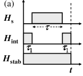
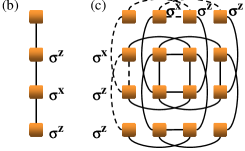
Figure 1: (a) Switching on/off the parts $H_{s}$ and $H_{\mathrm{int}}$ of the Hamiltonian $H=H_{s}+H_{\rm int}$ gives rise to an effective time evolution described by the stabilizer Hamiltonian $H_{\mathrm{stab}}$ [see Eq. (4)] whose ground state is a cluster state. (b) Graph representation of a one-dimensional 4-qubit (squares) cluster state stabilized by the Ising interaction. (c) Two-dimensional $4\times 4$ twisted cluster state stabilized by the $XY$ interaction, a universal resource for one-way quantum computation. The dashed lines and Pauli operators in each direction illustrate the twistedness of the state and the corresponding stabilizer Hamiltonian.

II.2 $XY$ model

Next, we show how to generate the stabilizer Hamiltonian using the $XY$ interaction, assuming that $H_{0}$ and $H_{\mathrm{int}}$ can be switched on/off independently.

The stabilizer Hamiltonian is formed step by step by bonding the nearest-neighbor operators. This is because the $XY$ interactions do not commute, $[[XY]_{i-1,i},[XY]_{i,i+1}]\neq 0$. We start from

$$e^{-i\theta[XY]_{12}}\sigma^{x}_{1}e^{i\theta[XY]_{12}} = \cos(2\theta)\sigma^{x}_{1}-\sin(2\theta)\sigma^{z}_{1}\sigma^{y}_{2},$$

$$e^{-i\theta[XY]_{12}}\sigma^{y}_{1}e^{i\theta[XY]_{12}} = \cos(2\theta)\sigma^{y}_{1}+\sin(2\theta)\sigma^{z}_{1}\sigma^{x}_{2},$$

$$e^{-i\theta[XY]_{12}}\sigma^{z}_{1}e^{i\theta[XY]_{12}} = \cos^{2}(2\theta)\sigma^{z}_{1}+\sin^{2}(2\theta)\sigma^{z}_{2}$$ (8)

$$+ \frac{1}{2}\sin(4\theta)[\sigma^{x}_{1}\sigma^{y}_{2}-\sigma^{y}_{1}\sigma^{x}_{2}]\>.$$

For $\theta=\pi/4$, these transformations increase the order of the Pauli-matrix terms as $\sigma^{x}_{1}\rightarrow-\sigma^{z}_{1}\sigma^{y}_{2}$ and $\sigma^{y}_{1}\rightarrow\sigma^{z}_{1}\sigma^{x}_{2}$. For $\sigma_{1}^{z}$ one obtains $\sigma^{z}_{1}\rightarrow\sigma^{z}_{2}$.

We now show how to construct a 2D stabilizer Hamiltonian. First we construct the 1D stabilizer Hamiltonian, starting from

$$H_{\rm s}=\Omega(-\sigma_{1}^{x}+\sigma_{2}^{y}-\sum_{i=3,N-2}\sigma_{i}^{x}+\sigma_{N-1}^{y}-\sigma_{N}^{x})\>.$$ (9)

In the specific case of six qubits in 1D, by applying Eq. (8) to $[XY]_{12}$, $[XY]_{34}$, and $[XY]_{56}$, we obtain:

$$e^{-iS_{1}}H_{\rm s}e^{iS_{1}} = \Omega(\sigma^{z}_{1}\sigma^{y}_{2}+\sigma^{z}_{2}\sigma^{x}_{1}+\sigma^{z}_{3}\sigma^{y}_{4}+\sigma^{z}_{4}\sigma^{y}_{3}$$ (10)

$$+ \sigma^{z}_{5}\sigma^{y}_{6}+\sigma^{z}_{6}\sigma^{y}_{5})\>,$$

where $S_{1}=\frac{\pi}{4}\sum_{l=1,3}[XY]_{\{2l-1,2l\}}$. Repeating this step with $S_{2}=\frac{\pi}{4}\sum_{l=1,2}[XY]_{\{2l,2l+1\}}$, we get the 1D stabilizer Hamiltonian $H_{\rm 1D}=e^{-iS_{2}}e^{-iS_{1}}H_{\rm s}e^{iS_{1}}e^{iS_{2}}$ that reads explicitly

$$H_{\rm 1D} = \Omega(\sigma^{z}_{1}\sigma^{z}_{2}\sigma^{x}_{3}+\sigma^{z}_{3}\sigma^{x}_{1}+\sigma^{z}_{2}\sigma^{z}_{4}\sigma^{x}_{5}+\sigma^{z}_{5}\sigma^{z}_{3}\sigma^{x}_{2}$$ (11)

$$+ \sigma^{z}_{4}\sigma^{x}_{6}+\sigma^{z}_{6}\sigma^{z}_{5}\sigma^{x}_{4})\>.$$

This Hamiltonian is twisted in the sense of tana , i.e., the site indices of the corresponding cluster state are obtained by the permutation $(2,3)(4,5)\ldots(N-2,N-1)$ (cyclic notation), for a chain of $N$ qubits where $N$ is even, see Fig. 1(b,c).

The next step in the construction of the 2D stabilizer Hamiltonian is to construct a ladder Hamiltonian by bonding nearest-neighbor sites on adjacent chains $a$ and $b$, in which all the bondings between qubits $ia$ and $ib$ are carried out simultaneously:

$$H_{\rm ladder} = \Omega(-\sigma^{z}_{1a}\sigma^{z}_{2a}\sigma^{z}_{b3}\sigma^{y}_{3a}-\sigma^{z}_{3a}\sigma^{z}_{1b}\sigma^{y}_{1a}$$ (12)

$$- \sigma^{z}_{2a}\sigma^{z}_{4a}\sigma^{z}_{5b}\sigma^{y}_{5a}-\sigma^{z}_{5a}\sigma^{z}_{3a}\sigma^{z}_{2b}\sigma^{y}_{2a}-\sigma^{z}_{4a}\sigma^{y}_{6a}\sigma^{z}_{6b}$$

$$- \sigma^{z}_{6a}\sigma^{z}_{5a}\sigma^{z}_{4b}\sigma^{y}_{4a})+(a\leftrightarrow b)\>.$$

A 2D stabilizer Hamiltonian is produced by connecting the above two ladder Hamiltonians with the interaction between the two ladders. For example, when we prepare two ladders of length 4 such as in Fig. 1(c) and connect them vertically, we obtain a $4\times 4$ stabilizer Hamiltonian.

II.3 Heisenberg model

For the Heisenberg interaction, we can construct only a two-qubit stabilizer Hamiltonian (note that the same is true for the $XXZ$ interaction). The basic relation is

$$e^{-i\theta[XYZ]_{12}}\sigma^{y}_{1}e^{i\theta[XYZ]_{12}}=\cos^{2}(2\theta)\sigma^{y}_{1}$$

$$+\sin^{2}(2\theta)\sigma^{y}_{2}+\frac{1}{2}\sin(4\theta)(\sigma^{x}_{1}\sigma^{y}_{2}-\sigma^{y}_{1}\sigma^{x}_{2})\>.$$ (13)

For the Ising and $XY$ models, we can eliminate the single Pauli matrix terms leaving the interaction terms [see Eqs. (5) and (8)]. However, in Eq. (13), if we set $\sin(2\theta)=0$ or $\cos(2\theta)=0$, we also eliminate the $\sigma^{x}_{1}\sigma^{y}_{2}-\sigma^{y}_{1}\sigma^{x}_{2}$ term. This is because the Heisenberg interaction contains terms in all three spatial directions tana . In the case of two qubits, we obtain $H=\Omega(\sigma^{z}_{1}\sigma^{x}_{2}-\sigma^{x}_{1}\sigma^{z}_{2})$ from the initial Hamiltonian $H_{s}=\Omega(\sigma^{y}_{1}-\sigma^{y}_{2})$ by using Eq. (13) for $\theta=\pi/8$. By applying a $\pi$-rotation, we obtain the two-qubit stabilizer Hamiltonian $H=\Omega(\sigma^{z}_{1}\sigma^{x}_{2}+\sigma^{x}_{1}\sigma^{z}_{2})$.

III Manipulation of always-on Hamiltonian

The scheme discussed up to now relies on switching on/off the single-qubit Hamiltonian $H_{0}$ [see Eq. (2)] and the Ising or $XY$ interaction part $H_{\rm int}$ separately. There is a number of schemes for switching on/off interactions between qubits (see, e.g., averin_bruder ; Nakamura ; nori ). However, they make the system more complicated and require additional overhead.

Here, we solve this problem by demonstrating how to extract $H_{0}$ and $H_{\rm int}$ by using appropriate pulse sequences. We illustrate the idea using the standard NMR Hamiltonian $H_{\rm nmr}=\sum_{i}\varepsilon_{i}\sigma_{i}^{z}+\sum_{i}J\sigma_{i}^{z}\sigma_{i+1}^{z}$ which has the property that $[H_{0},H_{\rm int}]=0$. In this case, $H_{0}$ and $H_{\rm int}$ can be switched on/off by using a simple pulse sequence. The interaction part $H_{\rm Ising}$ can be extracted by using two sandwiched $\pi$-pulses such as $\exp(i\tau H_{\rm Ising})=e^{-i(\pi/2)\sum_{j}\sigma_{j}^{y}}e^{i(\tau/2)H_{\rm nmr}}e^{i(\pi/2)\sum_{j}\sigma_{j}^{y}}e^{i(\tau/2)H_{\rm nmr}}$. On the other hand, two steps are required to obtain $H_{0}$. Let us consider a 1D qubit chain. By applying a $\pi$-pulse about the $x$-axis (denoted by $(\pi)_{x}$) to all the qubits on the even sites, we obtain $e^{-i(\pi/2)\sum_{i}\sigma_{2i}^{y}}e^{i(\tau/2)H_{\rm nmr}}e^{i(\pi/2)\sum_{i}\sigma_{2i}^{y}}e^{i(\tau/2)H_{\rm nmr}}=e^{i\tau\sum_{i}\Omega\sigma_{2i-1}^{z}}$. Similarly, we obtain $e^{i\tau\sum_{i}\Omega\sigma_{2i-1}^{z}}$ by applying a $(\pi)_{x}$-pulse to all the qubits on the odd sites. Combining these two processes yields $H_{0}$. This method is easily generalized to 2D or 3D qubit arrays.

If $[H_{0},H_{\rm int}]\neq 0$, this NMR method cannot be used. Even in this case, $H_{0}$ and $H_{\rm int}$ can be extracted separately. The idea follows from average Hamiltonian theory which is based on the Baker-Campbell-Hausdorff (BCH) formula for the expansion of $e^{A}e^{B}$ Ernst . A stroboscopic application of the Hamiltonian designed by a series of short pulses can reduce or eliminate unwanted terms, if $\Omega\tau,J\tau\ll 1$. First we extract $H_{\rm int}$ by setting $A=h_{0}+h_{1}$ and $B=-h_{0}+h_{1}$ in the BCH formula, where $h_{0}\equiv H_{0}\tau$ and $h_{1}\equiv H_{\mathrm{int}}\tau$. $B$ is realized by applying a $(\pi)_{y}$-pulse on every qubit. From the BCH formula, we obtain

$$e^{A}e^{B}\approx\exp(2h_{1}+[h_{0},h_{1}]+\frac{1}{3}[h_{0},[h_{0},h_{1}]])\;.$$ (14)

The exponent corresponds to a third-order expansion in $\Omega\tau$ for $\Omega\tau\ll 1$. If we repeat this operation $n$ times like $e^{A}e^{B}e^{A}e^{B}\cdots e^{A}e^{B}=(e^{A}e^{B})^{n}$ such that $n\Omega\tau=\pi/4$, the $k$-th term is of order $[\pi/(4n)]^{k}$. Therefore, $H_{0}$ is canceled, and we obtain only $H_{\rm int}$ in this order. When we apply

$$e^{A}e^{B}e^{B}e^{A}\approx\exp(4h_{1}-\frac{5}{3}[h_{1},[h_{0},h_{1}]]+\frac{1}{3}[h_{0},[h_{0},h_{1}]])\>,$$ (15)

we can eliminate the second term in Eq. (14). In the limit $n\rightarrow\infty$ under the condition of $n\Omega\tau=\pi/4$, $H_{0}$ is exactly eliminated. The extraction of $H_{0}$ can be achieved analogously. Moreover, as shown in Waugh , if the $k$th-order term is the first nonvanishing correction, the decay rate $T_{2}$ of the qubit system is enlarged according to $T_{2}^{\prime}\propto T_{2}(k+1)!(T_{2}/t_{c})^{k}$ as long as $T_{2}>t_{c}$ where $t_{c}$ is the time required for each single step [$A$ and $B$ in Eq. (14)].

For the $XY$ model, we have to switch off subsets of $H_{\rm int}$ corresponding to $S_{1}$ and $S_{2}$, as discussed after Eq. (10). This is equivalent to choosing $A$ and $B$ appropriately: e.g., for the 1D chain, $A=H_{\mathrm{int}}=h_{1e}+h_{1o}$ and $B=h_{1e}-h_{1o}$ where $h_{1e}=J\tau([XY]_{23}+[XY]_{45}+[XY]_{67}+..)$ and $h_{1o}=J\tau([XY]_{12}+[XY]_{34}+[XY]_{56}+..)$. That means, $B$ is generated by applying $\pi$ pulses to qubits $2,3,6,7,10,11,...$.

Let us consider the 1D $XY$ model with $\varepsilon_{i}=0$ in Eq. (2). The following operation can be used to obtain $H_{0}$. (i) Applying a $(\pi)_{x}$-pulse to all the qubits on the even sites changes the sign of $\sum_{i}\sigma_{i}^{y}\sigma_{i+1}^{y}$. (ii) By further applying a $(\pi)_{y}$-pulse to the same subset of qubits, we obtain $B/\tau=\sum_{i}\Omega(\sigma_{2i-1}^{x}-\sigma_{2i}^{x})-\sum_{i}J[XY]_{i,i+1}$. As a result, we obtain $\Omega\sum_{i}\sigma_{2i-1}^{x}$. Repeating the same operations with the qubits on the odd sites, we obtain $\Omega\sum_{i}\sigma_{2i}^{x}$. For the Ising model, the process (i) is not required. For the Heisenberg model, the same procedure as in the case of the $XY$ model does not eliminate the term $J\sum_{i}\sigma_{i}^{z}\sigma_{i+1}^{z}$. Thus, additional similar steps are required to eliminate this term.

IV Robustness

Since a practical realization of these pulse sequences will not be free of imperfections, we now analyze the effect of pulse duration errors $\delta$. A central quantity will be the cluster-state fidelity $F_{\rm st}(\tau)=|\langle\Psi_{00...0}|U_{\tau}(\delta)|\Psi_{00...0}\rangle|^{2}$ where $U_{\tau}(\delta)=e^{-i\tau H_{\mathrm{stab}}(\pi/4+\delta/4)}$. In the Ising case, $H_{\mathrm{stab}}$ is given by Eq. (7), and an analogous equation in the $XY$ case.

Let us consider the 1D Ising case. For $\theta=\pi/4+\delta/4$, the first-order correction to Eq. (7) reads

$$H^{\prime}(\delta)=\frac{\delta}{2}\Omega\left[\sigma_{1}^{y}+\sigma_{N}^{y}+\sum_{1<i<N}\sigma_{i}^{y}(\sigma_{i-1}^{z}+\sigma_{i+1}^{z})\right]\>.$$ (16)

The effect of these terms is calculated from perturbation theory using the expressions for $\sigma_{i}^{\alpha}|\Psi_{00..0}\rangle$, where $|\Psi_{00...0}\rangle$ is the initial cluster state, generated e.g. as proposed in Ref. tana , and $\alpha=x,y,z$ Aschauer . The lowest-order expression of the cluster-state fidelity reads $F_{\rm st}(\tau)\approx\left[1+\Omega^{2}\tau^{2}\delta^{2}(N-1)/2\right]^{-2}$, and the correction scales with $\delta^{2}$ which is a signature of the robustness of our method.

The simplest and most powerful method to further reduce the effect of pulse imperfections is the symmetrization of the pulse sequence frequently used in NMR Ernst . We first note that Eq. (3) is equivalent to

$$\rho(0)\stackrel{{\scriptstyle\tau_{1}H_{\rm int}}}{{\longrightarrow}}\ \ \stackrel{{\scriptstyle\frac{\tau}{2}H_{0}}}{{\longrightarrow}}\ \ \stackrel{{\scriptstyle-\tau_{1}H_{\rm int}}}{{\longrightarrow}}\ \stackrel{{\scriptstyle-\tau_{1}H_{\rm int}}}{{\longrightarrow}}\ \ \stackrel{{\scriptstyle\frac{\tau}{2}H_{0}}}{{\longrightarrow}}\ \ \stackrel{{\scriptstyle\tau_{1}H_{\rm int}}}{{\longrightarrow}}\rho(t)\>,$$ (17)

where, as before, $\tau_{1}=\pi/(4J)$. The second half of this pulse sequence results in a perturbation term that has the opposite sign as compared to Eq. (16). Applying Eq. (14) leads to a cancellation of the first-order perturbation term. If the original interval length $\tau$ is divided into an even number $n$ of subintervals, $\tau=nt_{c}$, the perturbation term is replaced by $[H_{\mathrm{stab}},H^{\prime}]i\tau\delta/(4n)$, and the fidelity $F_{\rm sym}^{n}$ is given by $F_{\rm sym}^{n}\approx\left[1+\Omega^{4}(2\tau^{2}/n)^{2}\delta^{2}(N-1)/2\right]^{-2}$. Hence, the fidelity is improved, $F_{\rm sym}^{n}>F_{\rm st}$, if $n>2\Omega\tau$.

These perturbative results are complemented by exact numerical calculations of $F_{\mathrm{st}}(\tau)$ and the gate fidelity $F_{\mathrm{g}}(\tau)=2^{-N}\>|\mathrm{Tr}\>U_{\tau}^{\dagger}(0)U_{\tau}(\{\delta_{i}\})|$ for $\tau=\pi/(4\Omega)$ in systems with up to $10$ qubits. Here, $\delta_{i}$, $i=1,\ldots,N-1$ corresponds to the qubit pair $(i,i+1)$. In both the Ising and $XY$ case, we averaged these fidelities over 2000 random realizations of the $\delta_{i}$ taken from a Gaussian distribution with varying width $\sigma$. The results indicate that the method is rather robust even outside the regime where $\sigma$ is much smaller than $\pi/4\approx 0.78$. For instance, the $XY$-model calculation shows that $F_{\mathrm{st}}$ is bigger than $99\%$ for $\sigma\lesssim 0.04$, while $F_{g}$ can be bigger than $99\%$ even for $\sigma$ as large as 0.07. The comparison between the two models shows that the robustness in the $XY$ case (see Fig. 2) is somewhat better than in the Ising case.

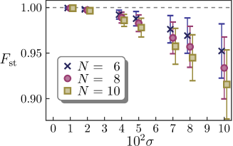
Figure 2: Dependence of the cluster-state fidelity for $\tau=\pi/(4\Omega)$ on random errors in the pulse duration for one-dimensional $XY$ qubit arrays of length $N=6$, $8$, and $10$. The width of the Gaussian distribution is denoted by $\sigma$; the error bars indicate the standard deviation.

V Discussion and conclusion

The distinguishing feature of the stabilizer Hamiltonians discussed here is that their ground states are directly related to the universal resource of measurement-based quantum computation. More generally, the stabilizer formalism has further applications in quantum information theory NielsenChuang . For instance, in quantum error-correcting codes Gottesman , the stabilizer formalism is used to express codewords. The method illustrated in Eq. (3) can be used to obtain eigenvalues for the syndrome measurements in the process of detecting errors. Moreover, relations (5) and (8) can be used to effectively generate codewords in solid-state qubits. For example, the three-qubit Greenberger-Horne-Zeilinger (GHZ) state $(|000\rangle\pm|111\rangle)/\sqrt{2}$, which is used for the nine-qubit code, is effective generated by $e^{\pm i(\pi/4)\sigma_{1}^{x}\sigma_{2}^{y}\color[rgb]{0,0,0}\sigma_{3}^{x}}|000\rangle$, where $e^{i(\pi/4)\sigma_{1}^{x}\sigma_{2}^{y}\color[rgb]{0,0,0}\sigma_{3}^{x}}=e^{i(\pi/2)(\sigma_{1}^{y}+\sigma_{3}^{y})}e^{\pm i(\pi/4)\sigma_{1}^{z}\sigma_{2}^{y}\color[rgb]{0,0,0}\sigma_{3}^{z}}e^{-i(\pi/2)(\sigma_{1}^{y}+\sigma_{3}^{y})}$ is applied to the three-qubit array. The five-qubit code Gottesman can also be generated by using this method.

To conclude, we have shown that initially prepared cluster states, e.g., 2D cluster states that are universal resources of measurement-based quantum computation, can be preserved with high fidelity. This is achieved by inducing the effective dynamics of 2D stabilizer Hamiltonians by means of specially tailored pulse sequences, starting from natural qubit-qubit interactions. We have also shown how this procedure can be implemented in the case of always-on interactions. Our work will facilitate implementations of one-way quantum computing.

References

• (1) For a review, see, e.g., H.J. Briegel, D.E. Browne, W. Dür, R. Raussendorf, and M. Van den Nest, Nature Phys. 5, 19 (2009).
• (2) H.J. Briegel and R. Raussendorf, Phys. Rev. Lett. 86, 910 (2001); R. Raussendorf, D.E. Browne, and H.J. Briegel, Phys. Rev. A 68, 022312 (2003).
• (3) M. Borhani and D. Loss, Phys. Rev. A 71, 034308 (2005).
• (4) T. Tanamoto, Y.X. Liu, X. Hu, and F. Nori, Phys. Rev. Lett. 102, 100501 (2009).
• (5) D.G. Angelakis and A. Kay, New J. Phys. 10 023012 (2008).
• (6) M. Van den Nest, K. Luttmer, W. Dür, and H.J. Briegel, Phys. Rev. A 77, 012301 (2008).
• (7) T.C. Wei, I. Affleck, and R. Raussendorf, Phys. Rev. Lett. 106, 070501 (2011).
• (8) F. Verstraete and J.I. Cirac, Phys. Rev. A 70, 060302 (2004).
• (9) S.D. Bartlett and T. Rudolph, Phys. Rev. A 74, 040302 (2006).
• (10) R.R. Ernst, G. Bodenhausen, and A. Wokaun, Principles of Nuclear Magnetic Resonance in One and Two Dimensions (Oxford University Press, Oxford, 1987).
• (11) J. Dinerman and L.F. Santos, New J. Phys. 12, 055025 (2010).
• (12) R. Heule, C. Bruder, D. Burgarth, and V.M. Stojanović Phys. Rev. A 82, 052333 (2010); Eur. Phys. J. D 63, 41 (2011); V.M. Stojanović, A. Fedorov, A. Wallraff, and C. Bruder, Phys. Rev. B 85, 054504 (2012).
• (13) D.V. Averin and C. Bruder, Phys. Rev. Lett. 91, 057003 (2003).
• (14) A.O. Niskanen, Y. Nakamura, and J.S. Tsai, Phys. Rev. B 73, 094506 (2006).
• (15) Y.X. Liu, L.F. Wei, J.S. Tsai, and F. Nori, Phys. Rev. Lett. 96, 067003 (2006); M. Grajcar, Y.X. Liu, F. Nori, and A.M. Zagoskin, Phys. Rev. B 74, 172505 (2006).
• (16) U. Haeberlen and J.S. Waugh, Phys. Rev. 175, 453 (1968).
• (17) H. Aschauer, W. Dür, and H.-J. Briegel, Phys. Rev. A 71, 012319 (2005).
• (18) M.A. Nielsen and I.L. Chuang, Quantum Computation and Quantum Information (Cambridge University Press, Cambridge, 2000).
• (19) D. Gottesman, Californian Institute of Technology, Pasadena, 1997, arXiv:quant-ph/9705052.