Hybrid Molecular Dynamics simulations of living filaments
Abstract
We propose a hybrid Molecular Dynamics/Multi-particle Collision Dynamics model to simulate a set of self-assembled semiflexible filaments and free monomers. Further, we introduce a Monte-Carlo scheme to deal with single monomer addition (polymerization) or removal (depolymerization), satisfying the detailed balance condition within a proper statistical mechanical framework. This model of filaments, based on the wormlike chain, aims to represent equilibrium polymers with distinct reaction rates at both ends, such as self-assembled ADP-actin filaments in the absence of ATP hydrolysis and other proteins. We report the distribution of filament lengths and the corresponding dynamical fluctuations on an equilibrium trajectory. Potential generalizations of this method to include irreversible steps like ATP-actin hydrolysis are discussed.
I Introduction
“Living” polymers form a class of supramolecular structures characterized by the reversible self-assembly of monomeric units into chains at equilibrium. greer-02 ; schoot-05 ; cates-06 ; cates-90 Some examples are systems forming discotic structures, bushey-01 ; keizer-04 fibrillar structures comprising of oligo(-phenylenevinylene) derivatives, jonkheijm-06 and wormlike micelles. rehage-91 Filamentous structures of proteins found in the cell, such as F-actin, korn-87 ; pollard-09 microtubules, desai-97 ; flyvbjerg-94 intermediate filaments alberts and bacterial pili sauer-00 ; kline-10 are usually coined as non-equilibrium polymers. howard Their assembly/disassembly properties are coupled to irreversible chemical steps, like the ATP/GTP (adenosine triphosphate/guanosine triphosphate) hydrolysis to ADP/GDP (adenosine diphosphate/guanosine diphosphate) within the filament complexes which act as catalysts. These complexes containing hydrolyzed nucleotides turn out to be more loosely bounded within the filaments. This leads to a shortening of persistence length for the hydrolyzed portions and to different critical concentrations at active ends. In contrast to the passive polymerization of equilibrium polymers, the active polymerization/depolymerization confers to these polar biofilaments unusual properties such as treadmilling where the filament grows at one end and shrinks at the other, or such as generation of work at the expense of chemical energy when a temporary network of filaments pushes on a membrane (e.g. in filopodia). faix-06 Numerous in vitro experiments have been conducted to observe and analyze various peculiar properties of biofilaments. Tubulin fibers have been observed to alternate between slow growth and catastrophe shrinkage sneppen-zocchi allowing for rapid reorganization of the cytoskeleton network while the role played by geometric boundaries on the growth dynamics of actin bundles was highlighted recently by Reymann et al. reymann-10
There have been several theoretical investigations based on mean-field stochastic models to study the contour length and composition dynamics of single free actin (also microtubule) filaments in presence of ATP hydrolysis. vavylonis-05 ; stukalin-06 ; ranjith-09 These theories have been adapted to investigate the behavior of bundles of filaments pushing against a flexible membrane gholami-08 or wall tsekouras-11 using straight and rigid filaments. They treat the free monomer concentration as homogeneous in space and constant in time and simplified hypotheses are assumed on the load distribution exerted by the surface on the filaments. Under conditions of confinement or crowding of bundles, it is expected that spatial correlations between filaments, their flexibility, the free monomer concentration fluctuations and the presence of local flows interfere with the main polymerization/depolymerization mechanism. To deal with more sophisticated situations where these aspects could be simultaneously taken into account, mesoscopic simulation approaches are needed. Pioneering Brownian Dynamics (BD) simulations, treating at the same time monomer diffusion and filament/network self-assembly, have been reported recently. They simulate actin networks pushing against an object lee-08 ; lee-09 or a long single actin filament undergoing (de)polymerization steps in presence of ATP hydrolysis. guo-09 ; guo-10
In this paper, we propose and develop a mesoscopic model to simulate a set of self-assembled semiflexible filaments within a statistical mechanical framework. The total number of filaments and the total number of monomers are both fixed in the simulations, leading to semi-grand canonical ensemble at equilibrium. The filaments are modeled according to a discretized version of the wormlike-chain with a variable contour length and an adjustable persistence length. The chemical reactive steps are simulated via a novel Monte-Carlo (MC) move which forms the core of the present work. This MC move which satisfies the micro-reversibility conditions, is specifically suitable to model single addition/removal of a monomer at the active ends of the semiflexible filament. It is reminiscent of the MC moves developed for modeling scission/recombination kinetics in flexible linear micelles huang-06 ; huang-09 or to model networks of reversible associating polymers hoy-09 in which operational parameters can be fixed to separately adjust the equilibrium constant and the barrier height for any reversible chemical reaction. In absence of any additional irreversible step, we get a model for a set of equilibrium semiflexible filaments in a well defined ensemble. All these modeling aspects are detailed in Section II. Section III covers the theoretical treatment of this system, starting with an ideal mixture treatment and looking then for packing effects on the filament size distribution and on the kinetic rates. Our simulation experiments are detailed and their results analyzed in Sections IV and V respectively. In the Section VI , we come back on some methodological issues and envisage the extension to non-equilibrium polymers which requires the consideration of monomer flags to distinguish between hydrolyzed and non-hydrolyzed ATP complexes and the consideration of additional chemical steps. The application of our methodology to a specific biofilament is discussed by providing the explicit parametrization which would be needed to model ADP-F-actin (homopolymer of ADP-actin complexes in interaction with free ADP-actin monomers). This is an interesting example, not found in vivo, of a polar equilibrium polymer where the polymerization and depolymerization steps take place at two kinetically inequal ends characterized by the same critical concentration. The paper closes with a short conclusion in Section VII.
II General mesoscopic model of a set of interacting living filaments and free monomers in a thermal bath
We first describe the detailed microscopic model of the solute/solvent bath system. Our simulation method consists of four parts: the adopted solute model for a mixture of free monomers and semiflexible filaments of various lengths (Section II.1), the solvent bath in which the solutes are immersed and the nature of the solute-solvent coupling (Section II.2), an original stochastic (de)polymerization procedure which, together with the solute model, defines the “living” filaments concept (Section II.3) and the statistical mechanics ensemble in which our finite-size system is sampled by our hybrid simulations (Section II.4).
II.1 The solute
The solute system treated throughout this work is a set of spherical monomers of mass . A fraction of these are present as free monomers. The remaining monomers constitute the building blocks of assembled polydisperse filaments with a range of sizes going from a minimum of three monomers to a maximum (set to an integer value ). The justification and the general consequences of imposed boundaries to the filament size will be discussed in Sections II.3 and II.4.
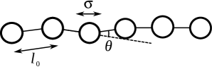
These filaments are modeled as semiflexible polymers with excluded volume interactions with its basic features adapted from a standard model. ripoll-05 ; padding-09 ; hinczewski-09 A schematic of the filament is shown in Fig. 1. Any filament with monomers has bonding interactions with an equilibrium length and an energy depth of
| (1) |
in terms of the absolute distance between adjacent monomers. The first purely vibrational term , where is the stretching force constant, maintains a chain structure with contour length . The second “electronic” term corresponds to a (negative) bonding energy with respect to a reference zero energy level corresponding to the large distance non-covalent pair energy between monomers, in order to favor the polymerization step (see Section II.3).
These non-covalent interactions are introduced via a shifted and truncated Lennard-Jones (LJ) potential, denoted by .
| (2) |
Here and are the energy and diameter parameters of the LJ potential. The Heaviside step function satisfies
| (3) |
Both intramolecular (beyond second neighbors) and intermolecular pairs are subject to such excluded volume interactions. Finally, a set of three-body potentials is used to favor the straight alignment of successive bonds () within each filament
| (4) |
where is the bending stiffness energy parameter, directly related to the persistence length according to .
Note that in applications of the model to filaments, one typically has and therefore, the short range (in physical distance) of the repulsive non-covalent interactions implies that the latter will usually not operate as “local interactions” but possibly as “long-range interactions” if the filaments are sufficiently long to behave as coils().
The particles trajectories are obtained by solving the Newton’s equations using the velocity-Verlet integrator, as in any standard Molecular Dynamics (MD) simulation.
II.2 The solvent bath
The system of monomers is immersed in a sea of solvent particles of mass treated according to the Multi-Particle Collisional Dynamics (MPCD) model. This technique, first introduced by Malevanets and Kapral, malevanets-99 ; malevanets-00 uses simplified solvent dynamics that faithfully reproduces the correct long time fluid behavior. Subsequent to its introduction, it has been extensively studied theoretically as well as being used to investigate various complex systems such as colloids, polymers and vesicles immersed in a solvent. gompper-09 Our use of this solute-solvent model, except for the living filaments aspects, is close to the semiflexible chains in solution. ripoll-05 ; padding-09
In this solvent model, all solvent particles move as free particles between (local) collisions taking place every time steps. The simulation volume is divided into cubic cells of side . The local collisions which take place independently in each cell imply velocity changes of all particles of the cell (solvent particles, free monomers and monomers pertaining to a filament) while preserving the total mass, linear momentum and energy of that cell. Explicitly, within each cell, the relative velocity of each particle (with respect to the cell subsystem center of mass velocity) is rotated by a fixed angle around a direction selected at random on a sphere with uniform probability.
Between the collision steps, the solute dynamics is followed by solving the equations of motion of the solute subsystem, treated independently of the solvent. This coupling enables the proper thermalization of the solute particles as well as the incorporation of hydrodynamic effects.
II.3 Modeling of (de)polymerization steps
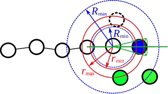
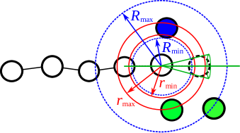
A fundamental property of bio-filaments such as actin, tubulin, pili etc., is their ability to grow/shrink via polymerization/depolymerization reactions at their ends. alberts We propose to model these chemical reactions as instantaneous events which modify locally the topological connections of the so-called “reacting monomer”. This change will be governed by a MC scheme, satisfying detailed balance, which is fully consistent with all the topological arrangements allowed by the semi-grand ensemble equilibrium partition function of monomers/filaments reacting mixture. Any instantaneous chemical reaction event taking place in our system will connect two microscopic states and differing only by the position of the single reacting monomer of (say index ) and by topological and geometrical constraints involving its link with the last monomer, (say of index ) of a particular active end of a filament and its immediate neighbor in the filament sequence (say index ). These three monomers which belong to the global set of solute monomers, are directly implied in the chemical step which we now describe with the help of Figs. 2 and 3 respectively representing the initial and final configurations of a polymerized or depolymerized state. In these figures, the dashed bead indicates the position of the unique reacting monomer in the alternative state.
In the polymerized state the reacting monomer, shaded dark blue in Fig. 2, is linked to the last monomer of the filament through a bonding potential and contributes to the bending energy term with monomers and . It is further imposed that in state , the polymerized monomer of index strictly lies within the region of low intramolecular energy volume determined as the intersection of two volumes: i) the conical volume whose symmetry axis coincides with the bond vector joining monomers and with its tip located at monomer having a tip angle , (ii) the spherical shell centered on the same monomer with inner and outer radii and . This volume amounts to
| (5) |
The limiting values and are chosen such that and the extreme cone angle is chosen such that . This implies that the volume is the locus of points in space where the incremental increase in vibrational potential energy remains a few .
In the depolymerized state , where the reacting monomer is shown in dark blue, it is still located close to the filament end monomer but is now free (in the sense that it only interacts with the filament end through excluded volume interactions). More precisely, to be in the depolymerized reacting state , the free reacting monomer must lie in a spherical layer centered on monomer with volume
| (6) |
where is such that and (namely twice the range of the potential in Eq. (2)).
We now envisage the energy modifications involved by the transitions between and by focusing on the incremental energy of the reacting monomer with respect to the rest of the system. In state , the total incremental energy, which contains both intramolecular and intermolecular contributions, can be written as
| (7) |
where the contributions from the stretching energy and the bending energy involving the reacting monomer have been regrouped into . The sum of all excluded volume pair interactions between monomer and the rest of the system is written as .
The total incremental energy of monomer in state is the sum of all its excluded volume pair interactions with the rest of the system (at a different location in comparison with state ), giving
| (8) |
Our chemical step model is best expressed in terms of reactive monomers. During the course of the simulation, any free monomer in the vicinity of the active end of a filament, i.e. located within the spherical layer of size centered on the end-monomer of the filament, will be coined as “free reactive monomer” meaning that it is susceptible to polymerize from a -type depolymerized state. Note that the reactive end of a filament is active unless the filament has reached the maximum size of monomers, in which case it can only depolymerize.
Similarly, the last monomer at the active end of a filament containing a minimum of four monomers (trimers are not allowed to dissociate as filaments must have at least three monomers) will be considered as a reactive end-monomer, i.e. susceptible to depolymerize from an -type polymerized state, as long as it is located within the low intramolecular energy volume .
During the time window in which a particular monomer is reactive, it can be the object of a chemical step. The occurrence of such an event being sampled in a Poisson distribution of times with nominal frequencies fixed (for reasons which will be justified later) to
| (9a) | ||||
| (9b) | ||||
The frequency prefactor is a free parameter which can be used to tune the trial frequencies (to tune the effective barrier height of the reaction) and hence the chemical rates in the system without affecting the equilibrium state.
When a chemical step involving a particular reactive monomer is selected by Poisson sampling statistics to occur at a specific time , depending on the nature of the reactive monomer, an MC attempted move () or () is made by sampling its new position uniformly from the volume or relative to the new or state. This new configuration is then accepted or rejected on the basis of an acceptance probability chosen to be
| (10a) | ||||
| (10b) | ||||
where . In practice, an explicit sampling of this acceptance probability finally decides the success of the chemical step at the time originally decided from the Poisson samplings of reaction times. When the chemical step is accepted, the reacting monomer is instantaneously and definitively transferred to its new location and topological status while keeping its linear momentum unaltered. The dynamical trajectory is then continued for times greater than on the basis of the new microscopic state dynamical variables. On the contrary, if the attempted chemical step is not accepted, no reaction is recorded and the reactive monomer simply follows, with the rest of the system, the dynamical trajectory it would have followed in the absence of any chemical step at time .
We note that finally, whether a chemical step is finally recorded or not, the reactive monomer remains reactive as long as it has not diffused out of the relevant or reactive volume in which it lies at times just later than . This point illustrates the coupling between monomer diffusion and reactive events. It indicates that the effective kinetic rates will not be strictly proportional to at high frequencies as a too large value of the attempt frequencies will necessary lead to ineffective sequences of polymerization/depolymerization steps involving the same filament end and reactive monomer.
The justification of the above Poisson/MC algorithm to deal with (de)polymerization steps requires the proof that it satisfies detailed balance at equilibrium for any pair of specific microscopic states (,). This can be seen easily by considering the ratio of the number of transitions between the two states and which can be expressed as
| (11) |
where both the numerator and the denominator contain four factors equal or proportional respectively to (i) the probability to be in the starting microscopic state or , (ii) the probability per unit time to make an attempt starting from the original state towards the alternative state of the reactive monomer, (iii) the probability to reach the specific final microscopic state in or in in the attempted move and finally (iv) the probability to accept this final state, hence to record a successful chemical step. To verify that the above ratio is unity, one simply needs to envisage explicitly two cases, whether the combination is positive or negative. Making it explicit for the former case, use of Eqs. (7), (8), (9) and (10) leads to
| (12) |
where (or similarly for ) denotes the total incremental energy of the reacting monomer in state . We note that alternative schemes are possible. However we observed that the present one maximizes the acceptance probabilities and thus optimizes the efficiency of the algorithm.
The MD algorithm is a step by step procedure where is the MD time step and (usually chosen such that where is an integer) is the time interval between two successive stochastic collisions in the MPCD procedure. The chemical reactions are integrated to the hybrid MD/MPCD scheme in the following way. At any discrete MD time , we make an exhaustive list of reactive monomers. This consists of filament-end monomers as well as free monomers which may appear more than once (in the list) if they are active with respect to more than one filament end. Then the occurence of each reactive step or during the next time interval between and is independently sampled by taking a random number from a uniform distribution between and and compared to or to . Any detected occurence is recorded. In most cases, after scanning the full list of potential reaction steps, we find zero or one occurence: in the latter case, the chemical step algorithm is applied at time until final MC acceptance or rejection of the new location and new topological link of the reactive monomer. In practice, we have never observed more than two occurrences during a MD step and in the rare double occurence cases, we attempt the reactions in succession.
II.4 Simulation ensemble including chemical reactions
Theoretical developments and simulation experiments will be performed in the ensemble in which, besides the volume () and the temperature (), the total number of monomers and the total number of filaments are both independently fixed. This ensemble is subjected to the additional constraint that the filament size, expressed in number of monomers, is restricted between a minimum of three and a maximum of . To any macroscopic state specified by a set of fixed thermodynamic variables, there will correspond an equilibrium free monomer number density and a filament length distribution which depends on the set of equilibrium constants associated to the relevant (de)polymerization steps connecting filaments of length and . Dynamic fluctuations at equilibrium involve various diffusive and reactive aspects which are in principle also species dependent. Considerable simplification occurs if the equilibrium constant can be treated as filament size independent. The length distributions then become simple exponentials and the concept of (an overall) average polymerization rate, , per active filament-end and the corresponding average depolymerization rate per active filament-end can be employed. In a subcritical regime () or in the supercritical regime (), the length distribution must be respectively a decreasing or an increasing function of the filament’s size, as a result of detailed balance. The ratio is equivalent to the ratio between the actual free monomer density and the state point dependent reference (“critical”) density, . This ratio directly indicates whether the state point is subcritical () or supercritical (). Within an ideal solution treatment, an independent equilibrium constant turns out to be a function of only the temperature, say , and a concentration independent critical density more directly separates subcritical () and a supercritical () concentration regions.
We close this section with some considerations about our choice to impose maximal and minimal bounds to the filaments in the context of living biofilaments, subject to single monomer polymerization or depolymerization. The presence of a lower bound to the size of existing filaments and the absence of consideration of any explicit nucleation mechanism imply that the number of filaments is strictly constant and fixed by initial conditions. As biofilaments are often generated by initiator proteins (like profilin for F-actin pollard-03 ) in vivo and in vitro biomimetic experiments, the imposition of a lower bound size in our simulations can be interpreted as a way to link the number of filaments to a fixed number of permanently active initiators. The imposition of an upper bound to the filament length follows primarily from our wish to treat living biofilaments in a simulation box for a broad range of equilibrium conditions, both in subcritical and supercritical conditions. In the former case, the upper-limit will have marginal effects if is large with respect to the characteristic size associated to the decaying exponential distribution. An equilibrated situation in supercritical conditions cannot be maintained with free living filaments as they would grow indefinitely. A stationary distribution is only possible if some confinement effect stops the unlimited growth of filaments. The upper limit should thus be seen as a simplified way to impose a confinement constraint allowing the establishment of the equilibrium state in supercritical conditions, a situation after all symmetric of the role of the lower bound (three monomers) in subcritical conditions. We finally note that in simulations, it will be pragmatic to adjust the size of the box such that the maximum length of the filaments satisfies .
III Theoretical framework
We provide below some theoretical predictions on the filament length distribution and on the dynamics of filament length fluctuations for the equilibrium system at fixed temperature described in the previous section. Our system consists of living filaments with size restricted between lower and higher bounds, subject to single monomer (de)polymerization steps at imposed total monomer number density and fixed global filament number density. The theoretical framework provides the tools for a consistency check of our hybrid MD simulation technique by comparing in the next section the results of simulation experiments at various state points with the theoretical predictions. We start by approaching the filament distribution at a macroscopic level but rely to statistical mechanics to discuss the microscopic expressions of the equilibrium constants. The second part of this section deals with the time evolution of the filament length populations on the basis of kinetic equations adapted to our system and we provide the microscopic expressions of these chemical rates.
III.1 The filament length distribution and equilibrium constants
Restricting ourselves to equilibrium, we denote the free monomer density by and the filament densities by . The constraints on the system are
| (13) |
and
| (14) |
where and are respectively the fixed monomer and filament global densities.
Chemical equilibrium requires that for each (de)polymerization reaction (implying filaments of length and and a monomer), the chemical potentials of the different species satisfy which can be transformed into an expression relating densities
| (15) |
where the equilibrium constant is a state point dependent quantity. Under the reasonable assumption that these equilibrium constants beyond the trimer () can be treated as independent of the filament size, the individual equilibrium densities can be expressed explicitly in terms of a unique constant which then turns out to carry the whole state point dependence of the distribution.
Applying recursively and combining with Eqs. (13) and (14), one gets an implicit expression linking the monomer density and ,
| (16) |
and an expression for filament densities in terms of and ,
| (17) |
Analytical expressions corresponding to Eqs. (16) and (17) can be obtained. Using reduced densities , and to simplify expressions, we exploit the properties of finite geometrical series (note that is finite and continuous around for non negative and finite) and . Equations (16) and (17) can then be rewritten as
| (18) |
and
| (19) |
where and .
The average size of the filaments in terms of monomers is then given by
| (20) |
Let us stress that Eqs. (18)-(19), shown respectively in Figs. 4 and 5, can alternatively be established via a statistical mechanics route (see Appendix A). A semi-grand canonical ensemble with similar constraints takes into account all possible arrangements of monomers distributed into filaments and remaining free monomers, at fixed volume and temperature. Such an approach is richer as it allows the calculation of additional properties like the composition fluctuations in finite systems. Let us further point out that Eqs. (18)-(19) are not closed equations, unless can be established separately. The reduction factor () being generally state point dependent, the above relations are not universal curves. They merely represent consistency relationships between , and , for an arbitrary state point specified by (, , ).
The free monomer density which corresponds to is known as the critical density. If an explored state point in our ensemble accidently yields , all filament length densities are equal, as seen in Eq. (19), and . As discussed in the next subsection on the dynamics of the filament length, the polymerization and depolymerization steps are then equiprobable and each filament performs a one-dimensional (1D) discrete random walk bounded from below at and from above at .
For an arbitrary state point, will differ from unity. If (supercritical conditions), the filaments are subject to a similar but biased bounded random walk where polymerization steps are more frequent than depolymerization steps (except for ) and the stationary filament length distribution is an increasing function of the length in order to satisfy detailed balance. The opposite situation is observed for subcritical conditions, as . Figures 4 and 5 illustrate respectively the equilibrium relationship Eq. (18) and the distribution Eq. (19). Equation (18) for finite upper bound cannot easily be inverted and must be solved numerically.

Provided , the limit of the upper value of the filament range can be taken in Eqs. (18), (19) and (20) which simplify respectively to
| (21) | ||||
| (22) | ||||
| (23) |
Here Eq. (21) can now be inverted to yield
| (24) |
All of the above expressions starting with Eq. (16), in particular the exponential distribution of filament sizes in Eq. (19), apply to equilibrium situations where the various chemical (de)polymerization steps are characterized by a unique (size independent) equilibrium constant . Such a simplified macroscopic approach will be found to be fully relevant to our model system. Therefore, we now exploit standard statistical mechanics expressions of the equilibrium constants, first within an ideal gas approach and then within a dilute solution approach where interaction effects, between filaments and monomers, are included at the second virial coefficient level.
III.1.1 Ideal solution
We first consider an ideal solution case, reminiscent of the reacting ideal gas treated in standard books, hill-thermody ; mcquarrie where all interactions between filaments and free monomers are neglected, but where (de)polymerization steps nevertheless take place between the different (phantom) species, the filament + monomer solute system being coupled to a heat bath “solvent” at fixed temperature . In that case, the equilibrium number densities must satisfy the chemical equilibrium relationship
| (25) |
where , function of the temperature only, is related to single filament or single monomer canonical partition functions by hill-thermody
| (26) |
The right hand side (RHS) of Eq. (26) can now be derived analytically for our filament model Hamiltonian provided only vibrational intramolecular interactions and are considered. As discussed in Section II.1, such a situation is valid as long as , because the intramolecular “long-range” monomer-monomer interactions which in fact act only at short physical distances cannot contribute for slightly bending rods. Using Eqs. (1) and (4) for , the kinetic contributions cancel out and thanks to the independence of the individual vibrational contributions, one finds an independent equilibrium constant for the RHS of Eq. (26) to be
| (27) | ||||
| (28) |
Here , and
| (29) |
The derivation of Eq. (28) from Eq. (27) is exact and relatively straightforward, requiring the use the integral
| (30) |
In our simulations, the values of the intramolecular parameters are chosen such that individual bond lengths have negligible fluctuations () and filaments semiflexible (). Therefore, Eq. (28) of the equilibrium constant simplifies to
| (31) |
which more directly shows the impact of the model parameters on the equilibrium constant.
III.1.2 Effects of interactions
At this point, we introduce the activity coefficients and which measure for monomers and filaments of different lengths, the deviation from ideal behavior in the composition term of the chemical potential. In terms of these, the equilibrium constant associated to the reversible depolymerization of a filament of length can be expressed as hill-thermody
| (32) |
In Eq. (32), is a function of the thermodynamic state (and no longer a function of only the temperature). In presence of intermolecular forces, the dependence of for filaments is expected to be very weak while the magnitude of the intermolecular effects on , for our model filament model, should primarily be related to the change in covolume resulting from the addition or the removal of a monomer at the end of a filament. This point can be analyzed quantitatively within the framework of the low density expansion of the activity coefficients. In Appendix B, we obtain a first-order estimate of as
| (33) |
where the factors are the expansion coefficients of the pressure in powers of the activities of the various species in the mixture. These factors can be expressed as follows
| (34a) | ||||
| (34b) | ||||
| (34c) | ||||
| (34d) | ||||
where the pairs of indices imply corresponding two body interactions and the pair configurational integrals between species and are defined as
| (35) | ||||
| (36) |
In these expressions, and are one body canonical partition functions and and are two body canonical partition functions for different and similar bodies respectively.
To be specific in this calculation of the second virial coefficients, we treat our filaments as rigid rods and we concentrate on the expressions relevant to the first order term in in the expression given by Eq. (33). We have gray-gubbins
| (37) | ||||
| (38) |
where is the monomer-monomer pair potential and is the intermolecular potential between a filament of length with center of mass at the origin and with (arbitrary) fixed orientation and a free monomer located at . The explicit expressions of the corresponding factors are
| (39a) | ||||
| (39b) | ||||
These integrals can be estimated by approximating the free monomers as hard spheres of diameter and filaments as hard spherocylinders built as a cylinder of height and radius , terminated by two hemispheres of radius . Performing the integrals gives
| (40) | ||||
| (41) |
where and are the excluded volume of respectively a sphere or a spherocylinder, when approached by another sphere. Supposing that in Eq. (33) the monomer density is dominant with respect to the other terms involving filament densities, we get the net covolume effect on the equilibrium constant as,
| (42) |
This result gives at least the order of magnitude of intermolecular effects on the equilibrium constant and moreover suggests, as expected, that the dependent effects should be small.
III.2 Mean field rate equations and rate constants
III.2.1 Effective (de)polymerization rate constant
The (de)polymerization processes which take place within the system imply the following reaction
| (43) |
where represents a free monomer, a filament consisting of monomers and one with monomers. In the mean field kinetics model, the independent and are respectively the polymerization and the depolymerization rate constants for filaments undergoing reactions at their active ends. Chemical equilibrium implies that the mean field equilibrium constant , a function of the thermodynamic state, satisfies .
Let us first consider polymerization events in an equilibrium situation with densities . The combination expresses the number of polymerization steps per unit of time and per unit volume involving specifically filaments of length . In our general statistical mechanics model the filaments can only fluctuate between and . Accordingly, the mean of the total number of reactive pairs for polymerization per unit volume (at any time) is given by where the volume factor equals to
| (44) |
in terms of the equilibrium radial pair distribution between any filament active end and surrounding free monomers. In the ideal solution case, it simplifies to . According to our microscopic kinetic model, the total number of successful polymerization steps per unit volume and per unit time can be written as a product of three contributions, namely, the total number of reactive free monomers per unit volume, the polymerization attempt frequency Eq. (9b), and finally, the polymerization acceptance probability Eq. (10b). We thus have
| (45) |
Here the average runs over all polymerizing events sampled uniformly in the reacting volume . The incremental excluded volume energy of the reacting monomer in the different states or are represented by or . Also is the non-negative incremental vibrational energy of the reacting monomer in state obtained by grouping the stretching potential and the bending potential provided by Eqs.(1) and (4).
Now considering the depolymerization events at equilibrium, the average number of reactive (breaking) pairs per unit volume is given by where the factor is the fraction of end monomers at the active end of the filaments which lie in the reactive volume .
The total number of successful depolarization per unit of time and per unit of volume is, using depolymerization frequency Eq. (9a), and depolymerization acceptance probability Eq. (10a), given by
| (46) |
In this case, the average runs over depolymerizing events sampled uniformly in the spherical layer of volume .
To summarize, we finally get the rate expressions
| (47) | ||||
| (48) |
The order of magnitude of these rates for reasonably dilute solutions can be estimated by neglecting excluded volume interactions, using , and the ideal solution equilibrium constant given in Eq. (31), as
| (49a) | ||||
| (49b) | ||||
III.2.2 Mean-field filament length dynamics
The filament length dynamical evolution is usually treated theoretically in terms of a chemical master equation with the reaction rates treated as input constants. For biological filaments like actin, filaments change by one unit and, if we disregard for the present time the existence of variants in the complex formation of the monomers and the modification of ATP into ADP through hydrolysis, only the polymerization rate and the depolymerization rate are relevant for the single monomeric species considered. In our case where the filament lengths fluctuate between and , the set of equations governing population dynamics reads
| (50a) | ||||
| (50b) | ||||
| (50c) | ||||
where is the probability to observe filaments with length at time and in Eq. (50b) the index runs from up to . This set of equations is solved for constant rates and for given initial conditions . This approach which treats independent filaments is physically justified if the monomer density (apparently uncoupled to the dynamical scheme) is assumed to be homogeneous in space and in time. Well stirred systems with compensating external addition or removal of free monomers provide plausible non-equilibrium stationary conditions for which the set of Eqs. (50) is pertinent.
In our context we explore different specific values of and . The Eqs. (50) can be tested by our simulations if we probe the dynamical filament length fluctuations at equilibrium. For example, by picking up a subset of filament of length at some time and following the time evolution of their size distribution, one should get an evolution from the original delta function back to the equilibrium distribution. This distribution is simply the conditional probability that a filament having a length at an initial time has a length at time .
This conditional probability time evolution will reflect the statistical properties of the bounded biased random walk induced by the chemical steps. However, if the starting size is not immediately close to a boundary at or at , the behavior of will be representative of an unbounded biased random walk as long as the measuring time remains much smaller than the (shortest) mean first passage time towards one of the boundaries. At long times, boundaries have a major influence (in any subcritical or supercritical regime) on the re-establishment of the equilibrium distribution.
| Exp. | ||||||||
|---|---|---|---|---|---|---|---|---|
| G1 | 1076 | 0.0121 | 0.60658 0.004 | 0.12203 0.0002 | 0.12227 | 0.00244 | 0.00399 | 0.02000 |
| G2 | 1744 | 0.0196 | 0.91490 0.003 | 0.17994 0.0006 | 0.18009 | 0.00356 | 0.00389 | 0.01978 |
| G3 | 2008 | 0.0225 | 1.00756 0.001 | 0.19805 0.0003 | 0.19808 | 0.00388 | 0.00385 | 0.01959 |
| G4 | 2338 | 0.0262 | 1.13775 0.001 | 0.22141 0.0003 | 0.22168 | 0.00432 | 0.00379 | 0.01951 |
| G5 | 3311 | 0.0372 | 1.78321 0.008 | 0.33824 0.0002 | 0.33831 | 0.00637 | 0.00360 | 0.01883 |
| G6 | 4000 | 0.0449 | 2.39206 0.020 | 0.44891 0.0001 | 0.47836 | 0.00821 | 0.00345 | 0.01829 |
IV Adopted microscopic parameters and list of simulation experiments.
All the physical quantities will be expressed in a system of units based on: the length of the side of the cell in MPCD, the energy (where is the Boltzmann constant) and the mass of a solvent particle. The resulting time unit is expressed as .
For the monomer/filament model, we adopt a unique set of parameters inspired by previous works on semiflexible chains in MPCD solvent ripoll-05 ; padding-09 or in BD solvent hinczewski-09 , namely beads of mass with size and energy parameter . Within the filament, monomers are linked by hard springs with equilibrium length and force constant . The bending parameter is set to , which implies a persistence length of . These values lead to a reactive volume (see Eq. (6)) defined by (for which the potential is ), and , while those defining the reactive volume (see Eq. (5)) are given by , and rad.
The MPCD parameters are chosen to match a well studied state point, ripoll-05 given by a solvent density of , box collision angle of and a collision frequency . At this solvent state point, it is known that a particle of mass interacting at infinite dilution via MPCD collisions with solvent, has a diffusion coefficient ripoll-05 of so that an estimate of the diffusion time is (where is the distance where the potential ).
With the adopted kinetic parameters and one gets at , the ideal solvent equilibrium constant . This allows the estimates of rates, from Eqs. (49), as and respectively.
All the simulation experiments, conducted at a common temperature , follow filaments with size fluctuating between three and which are enclosed in a cubic volume containing MPCD solvent particles. Note that the box length () is twice the maximum allowed filament length. Periodic boundary conditions are applied in all three dimensions. Table 1 reports the total number of monomers which is specific to each experiment, together with experiment codes G1 - G6 increasing with and the associated volume packing fraction . In the simulations, the MD integration time step , associated to the Verlet algorithm, has been set to , which corresponds exactly to .
A typical simulation setup involves an equilibration run of corresponding to depolymerization steps per active filament end or to . Four runs of time duration of are then performed in succession to get four independent estimates of the averages of interest which are then used to determine the global average (over a total time of ) and an estimate of the associated statistical error.
V Simulation results
V.1 Equilibrium distributions
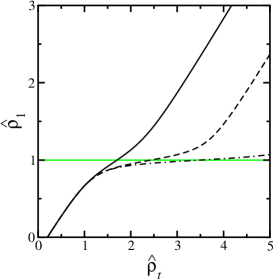
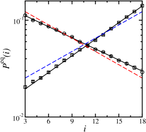
The experiments differing in the total number of monomers in the box lead to a resulting free monomer density (see Table 1) and a distribution of filament densities for all accessible lengths (monomer number). In all cases, the distribution of filament lengths turns out to be exponential, confirming the hypothesis of a unique (state point dependent) equilibrium constant for all filament lengths. In Fig. 6, (in log scale) versus (for two cases) is plotted. It shows a linear behavior with a slope providing directly the reduced free monomer density . All the data obtained from the filament distributions of the various experiments are gathered in Table 1. It shows that as increases, the system goes from subcritical to supercritical conditions, with the experiment G3 being very close to the critical situation. In Fig. 6, we also show the distribution expected (dashed lines) for the same state point () if ideal solution conditions were applicable with equilibrium constant computed from Eq. (31).
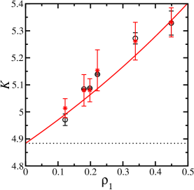
By dividing by for each line of the Table 1, one gets a first estimate of the equilibrium constant which is shown in Fig. 7, as a function of itself. We postpone the discussion of the increase of versus until we confirm these data with a second estimate of extracted from the number of chemical (de)polymerization steps in the next subsection.
V.2 State point dependence of rates and related equilibrium constant
The effective rates and can be estimated, on the basis of the assumption that they are independent of filament length, using expressions in Eqs. (45) and (46). The quantities and in these expressions are obtained by the counting of the total number of successful polymerization and depolymerization steps observed during the simulation, divided by the volume and the total simulation time. The rates for the six experiments are gathered in the Table 1 and are also reported in the Fig. 8.
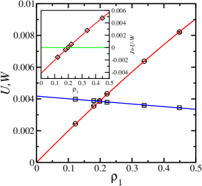
We observe that slightly decreases with increasing , a property which must be related to a decrease in the rate of acceptance of an attempted depolymerization step due to higher packing density. Similarly, the polymerization rate is not strictly linear in and a negative quadratic term can be extracted from a fit. We perform the three parameters combined fit and as we impose that for , the ratio of and reproduce the thermodynamic value of . We find , and . To first order, it gives the relationship with . This value can be compared with the theoretical prediction given by Eq. (42), which gives if the size of the monomer is taken to be equal to the distance at which the energy is of the order of unity (). The estimate has the correct order of magnitude but is about too low perhaps because the covolume effects of the filaments are included in the fitted quantities ( and ) but are absent in the theory. We believe however that the main source of increase of the equilibrium constant with finds its origin in the covolume effect described in Eq. (42).
V.3 Dynamic fluctuations of filament length
At equilibrium, we consider the (static) population probability ) and the conditional probability for a filament to have a length at time if its length was at time . In terms of these, one can express the time correlation function of filament length by
| (51) |
The normalized correlation function of the length fluctuations around their mean is formally
| (52) |
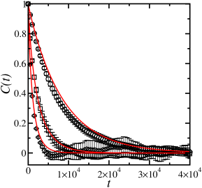
where and . Figure 9 shows the variation in with for the experiments G1, G3 and G5. These curves are in excellent agreement with the theoretical expressions of based on Eqs. (51) and (52) where the conditional probabilities are computed by solving the mean field population dynamics Eqs. (50), using the tabulated values of and at the same state point. We observe that the relaxation time of these fluctuations is maximum at critical density (experiment G3), as a result of the uniform distribution of filament lengths which requires a filament to explore a wide range of lengths before loosing memory of its initial value.
In Fig. 10, we observe the growth or decay of the length of filaments in various super or subcritical regimes, focusing on the short time behavior of the conditional probabilities for particular filament lengths which are present in reasonable number and located relatively far from the boundaries at three or at the same time zero.

The quantity measured and shown in Fig. 10 is
| (53) |
and is also averaged over a few appropriate filament lengths. Since the largest (de)polymerization rates are of the order of , it can be expected that for times , the filament populations of for or are still negligible and the behavior of is representative of a situation at the same density of unbounded filaments. We have verified that the slopes of the straight lines observed in Fig. 10 are in full agreement with the global growth or decay rate shown in the inset of Fig. 8.
VI Discussion
The methodology presented in this work applies to the sampling of a reactive (semi-grand) canonical ensemble consisting of a mixture of free monomers and a fixed number of self-assembled linear polymeric filaments. Specifically, the filaments undergo reversible single monomer end-filament polymerization/depolymerizations at one or both active ends of any filament. Regarding the filament model, a discretized wormlike chain is used as the basis of an extension towards a “living wormlike chain” version where the contour length is variable. In this section, we mention some specific details of our method, some of them with respect to alternative approaches proposed in the literature. We briefly indicate how our methodology can be generalized to include additional or alternative kinetic processes found in biofilaments such as filament rupture, distinction between ADP and ATP complexes and irreversible hydrolysis processes. We organize this discussion by regrouping some purely methodological aspects first, and then consider the explicit case of actin to illustrate the versatility of our approach.
VI.1 Methodological aspects
The dynamic trajectory of our solute (reactive mixture of filaments and free monomers), coupled to a bath of solvent particles, is obtained via a numerical scheme which incorporates MC reactive steps in the hybrid MD-MPCD method. For non-reacting fluids, the hybrid algorithm conserves the total energy but in our case, the MC chemical steps give an overall canonical ensemble character to the sampling. The imposed canonical temperature is set in the acceptance probabilities of the chemical step Eqs. (10) and in the attempt depolymerization frequency Eq. (9a)). Between two successive chemical events, the system’s total energy is conserved but it is discontinuous when a chemical step is successful. Pragmatically, the initial equilibration run to probe a new state point is started with initial velocities for solute monomers and solvent particles such that the average kinetic energy per degree of freedom is set equal to . As the system equilibrates while undergoing chemical steps at the same prescribed temperature, the instantaneous average kinetic energy per degree of freedom fluctuates in time around the expected stable value. The choice of coupling of the new chemical steps proposed in this paper to a MPCD solvent may be questioned. This (continuous space) particulate description of the solvent locally conserves momentum and hence preserves long wavelength fluid hydrodynamics as well as allows the boundary conditions to be easily adjusted. This may play an important role in highly confined geometries such as in biofilaments in a microchannel or actin bundle developments in filopodia.
The stochastic scheme to model the (de)polymerization steps is a purely instantaneous local perturbation. This is meant to represent at a mesoscopic level (coarse graining in space and time), the direct coupling effect of many internal and external degrees of freedom of the reacting pair “filament end”-“protein complex” which are eliminated. The modeling of the chemical step introduces a local discontinuity in the position of the reacting monomer but not in the monomer velocity. This is the price to be paid in order to succeed in devising a scheme in which the free reacting particle can be effectively moved to/from a position in space where it participates with the other degrees of the filament to an equilibrated intramolecular configuration. In real systems, as one protein binds to an existing protein filament in solution, it requires some time to modify its internal structure, to adjust its orientation and its translational location so that intermolecular interactions between units stabilize the newcomer. This waiting time corresponds in our model to the sampled reaction time in the Poisson process governed by the attempt frequency in Eqs. (9), which can be tuned via the free parameter . The reactive steps are modeled as local events obeying micro-reversibility. They are effectively coupled to the solute degrees of freedom through structural properties like the filament end-monomer/free-monomer pair correlation function, and through the various filament and free monomer diffusive processes. Our simulation results indicate a weak variation of the rates with state point at moderate solute packing fractions when the effective kinetic rate constants are computed for a fixed set of parameters regarding the stochastic model (reacting volumes and , and attempt frequency ). We have pointed out that the order of magnitude of the rates can be estimated from the ideal solution behavior (Eqs. (49)).
There is a large amount of literature on simulation methods/studies of flexible or semiflexible equilibrium polymers but most of them resort to various purely MC schemes which sample a grand-canonical ensemble (with addition/removal of individual molecules homogeneously in the simulation box) subject to additional constraints on chemical potentials in order to impose chemical equilibrium, frenkel-smit ; lu-04 or use sometimes artificial MD schemes to compute only the equilibrium static quantities. lisal-06 Our exploration of the reactive semi-grand canonical ensemble by MD gives similar information on thermodynamic and structural quantities (such as distributions of filament length populations, various monomer/filament pair correlation functions etc), but in addition yields dynamic information on diffusive and reactive processes both at equilibrium, as illustrated in the present work, and potentially outside equilibrium.
Reaction-diffusion aspects of biofilaments (actin) in presence of explicit reactive free monomers have been studied recently in inspiring BD studies. lee-08 ; lee-09 ; guo-09 ; guo-10 The depolymerization steps are modeled as explicit end-monomer detachments directly triggered by an independent stochastic process with fixed depolymerizing rate. The polymerization step relies on the detection of free monomers entering, by diffusion, into a capture zone volume defined at the reactive end. Subsequent to its entry, the monomer is automatically treated as reactive and subsequently attached to the pre-existing flexible filament. In all these studies, the opposite polymerization and depolymerization steps do not satisfy micro-reversibility. While Lee and Liu lee-08 ; lee-09 studies are very specific and concerned with far from equilibrium network developments close to a moving disk (including branching and capping phenomena) to investigate the origin of disk motility, Guo et al., guo-09 ; guo-10 are concerned with more basic phenomena on single F-actin filaments regarding size and composition fluctuations. They treat a single unbounded filament surrounded by free Brownian monomers at a strictly constant concentration, mimicking an homogeneous stationary non-equilibrium situation. Purely ADP-actin complexes have been considered in the first study concerned with a stationary growth or shrinkage of the filament. In the next work, treadmilling has been produced by a similar BD study in presence of three types of actin complexes namely, ADP-, ADP+Pi- and ATP-actin. (Here Pi represents inorganic phosphate group). In these BD studies, for pragmatic reasons, chemical reactions are artificially accelerated with respect to a free monomer diffusive time scale of reference, by increasing both kinetic rates and free monomer concentration in order to follow diffusion and chemical events within a unique simulation time window allowing significant statistics on the slowest dynamical events. Our methodology is different but works at the same mesoscopic level and therefore, if applied to the actin case, it would face the same wide spectrum of time scales problem discussed above. Progress on further time-space rescaling needs to be envisaged such as considering the elementary monomeric unit treated in the model to represent a collection of a few ATP-protein and/or ADP-protein complexes, with an effective slower diffusion constant and adapted chemical steps.
Coming back to the large classes of equilibrium and nonequilibrium self-assembled polymers or filaments considered in the introduction, the kinetic processes which are involved in their self-assembly and disassembly are known to be of very different nature. Cylindrical micelles can break anywhere and reform by end-recombinations and this mechanism is potentially plausible to some extent in biofilaments also. bausch-11 Biofilaments are usually subject to ATP-hydrolysis while the building blocks of the filaments are ATP-protein complexes which can thus be transformed in other complexes when integrated into filaments. In our method, we only restrict the chemical steps to be single unit end polymerization or depolymerization and that too to single monomer species. Our approach can however be easily extended to cover all these cases as illustrated in the next section where we discuss some aspects of actin modeling.
VI.2 Parametrization of our generic biofilament model to F-actin
For illustrative purposes, we discuss below the application of our method to actin at the level of one free monomer particle being one single protein complex with ADP or ATP. Referring to the study of actin by Guo et al., guo-09 ; guo-10 we discuss in detail the parametrization needed in the equilibrium polymer case where any monomer, either free or integrated in a F-actin filament, remains permanently in the actin-ADP complex state. We then briefly discuss extension towards non-equilibrium actin filaments subject to irreversible ATP hydrolysis.
To begin with, we remark that the diffusion time of free monomers in our study, depending on the mass of the free monomer and various parameters of the MPCD solvent, turns out to be . This can be used to set the basic time unit as s when the experimental Globular-actin diffusion coefficient of m2/s is taken into account. mcgrath-98 The size of the monomer is , fixing our length unit to nm. As actin has a double-stranded helix structure, alberts it is usually in simplified models as a single strand such that each monomer addition increases the effective contour length of the filament by half the size of a unit. ranjith-09 This implies we should take . The force constant is not a sensible physical parameter but it should be fixed to a sufficiently large value to avoid unphysical fluctuations of the contour length. The bond fluctuations are small with respect to if the quantity defined in Eq. (28) satisfies . In the present discussion, we can keep the value in simulation units, as this value leads to . Next, we must fix such that we reproduce the experimental value of the persistence length of the pure ADP-F-actin at K which is m. isambert-95 This gives a value of . The value of the equilibrium constant will next be imposed in the model by using Eq. (31) valid as long as , and by exploiting the freedom in choosing the bonding energy parameter . We thus find in order to get the experimental critical concentration of M. fujiwara-07 These set of parameters still require the rate to be adjusted to match the experimental data of the off-rates (the on-rates are automatically satisfied if is correctly fixed). As one has different values at both ends, namely s-1 at the barbed end and s-1 at the pointed end, fujiwara-07 one gets by applying Eq. (49a), s-1 and s-1.
Moving now to F-actin filaments consisting of three different forms of complexes, namely ATP-actin, ADP+Pi-actin and ADP-actin, requires associating a flag to each monomer in the model. Any active end of the filament (“barbed end” or “pointed end”) may differ in monomer composition (hydrolysis status) and hence specific rate constants for each case must be adjusted in the model parameters. The kinetic model for the associated irreversible hydrolysis of the ATP form needs also to be specified, as well as the associated kinetic rates. To discuss the parametrization in this context, let us adopt a simplified treatment ranjith-09 where the intermediate form of ADP+Pi-actin is merged with the ADP-actin form so that only two distinct forms are retained and where the hydrolysis step, which irreversibly changes the ATP-complex in the filament into an ADP-complex, takes place only at the boundary of an ATP cap and pure ADP section (vectorial process). In such a block-copolymer, the different parameters , and for the ADP block at the pointed end (and at the barbed end in case the ATP cap has vanished) can be adjusted on those of the pure ADP case discussed previously. One can proceed in the same way for the ATP block adjusting the parameter to match its stiffer character (persistence length of 15-17 m gittes-93 ; ott-93 ) and further impose values of for the barbed end (and the pointed end in case the ADP block would have vanished) in order to match the corresponding experimental values of kinetic rates and hence of the equilibrium constants. Finally, an independent stochastic process with rate fixed to its experimental value would convert the first ATP-complex of the cap into the ADP form. Actin simulations would be run as explained in Section II but with a much large variety of reactive monomers including ATP (or ADP) barbed end (or pointed end) monomers, ATP monomers at the diblock boundary and ATP (or ADP) free monomers in the reactive volume centered on an active end (barbed or pointed). For the hydrolysis reaction, if sampled during a MD step, the reaction is automatically performed as an irreversible step. In all other cases where a monomer is selected to perform a specific reaction, an attempted MC move is performed which is then subject to the appropriate acceptance criterion.
VII Conclusion
To conclude, we have presented a hybrid MC-MD model to simulate living biofilaments in the framework of the widely used wormlike chain model, with reactive dynamics at the ends giving rise to contour length variations. We believe that our mesoscopic approach, being formulated within a statistical mechanics framework, could be the starting point for numerous applications and extensions. The study of the growth of filament bundles in free or in confined space are in progress. More generally, in the multi-scale problem of living biofilaments dynamics, our methodology offers a well defined model at an intermediate level which should open natural bridges to more atomistic models on one side and on the other side, to more coarse-grained models to be based on further systematic and controlled rescaling procedures. On a side note, our simulation approach could also be easily adapted to study polymer synthesis in good solvent by living polymerization, in particular, to follow the time evolution of the size distribution of the polymers. das-99
Acknowledgements.
The authors are grateful to Marc Baus, Ray Kapral, P. B. Sunil Kumar and Jean-Louis Martiel for illuminating discussions on various aspects of the work. We thank Georges Destree at the ULB/VUB Centre de Calcul for efficient programming support. SR wishes to acknowledge the BRIC (Bureau des Relations Internationales et de la Coopération) of the ULB, for financial support.Appendix A Statistical mechanics treatment
The partition function of our semi-grand canonical reactive ensemble treats independent solute entities divided into a set of living filaments with polymer size fluctuating through single monomer (de)polymerization between and and a set of free monomers such that the total number of monomers is fixed. It reads
| (54) |
where is the canonical partition function of a single filament of size or of a free monomer for . hill-thermody ; gubbins-94 Owing to the fluctuating size of the filaments between their lower and upper limits, the sum in the partition function involves all possible arrangements of monomers which satisfy the explicit constraints, jointly denoted formally as in Eq. (54),
| (55) |
and
| (56) |
In addition, we suppose that the state point equilibrium constant associated to monomer attachment to/detachment from a filament is independent of the filament size.
This theoretical treatment can be justified within two approaches which are both relevant to the interpretation of our simulation experiments involving interacting and reactive filaments:
- •
-
•
It provides an approximate treatment based on a mean-field approach whereby the partition function is written in terms of independent effective single filament partition functions . The and hence the related equilibrium constant supposed to be independent, are state point dependent. The state point dependence of needs to be approximated to close the set of density equations (see Eq. (42)).
The recursive application of Eq. (15) with gives so that the partition function can be rewritten as
| (57) |
The average number densities of monomers and filaments in the thermodynamic limit can be estimated hill-thermody by searching for the largest term of the partition function . This requires solving the constrained global minimum
| (58a) | ||||
| (58b) | ||||
where and are Lagrange multipliers related respectively to the constraints Eqs. (55) and (56). Use of the Stirling’s approximation leads to the set of equations
| (59) | ||||
| (60) |
In terms of reduced number densities , one gets
| (61) | ||||
| (62) |
The combination of Eqs. (56) and (62) gives , hence leading to the filament densities Eq. (17), while the implicit equation in free monomer density Eq. (16) follows by direct substitution of filament densities in the constraint Eq. (55).
Appendix B First-order estimate of equilibrium constant in the presence of excluded volume interactions
The pressure expansion of a mixture of monomers and filaments in terms of activities reads hill-thermody
| (63) |
where the activities are defined by
| (64a) | ||||
| (64b) | ||||
Here the coefficients are related to two-body integrals by Eqs. (34) and Eqs. (39). The number densities can then be expressed as
| (65) | ||||
| (66) |
In the above equations, the series are limited to quadratic terms in . These relations can be inverted by writing
| (67) | ||||
| (68) |
where the coefficients can be obtained by substitution of the latter expansions in the density expansions (Eq. (66)), followed by term by term identification, giving
| (69) | ||||
| (70) | ||||
| (71) | ||||
| (72) |
Using Eq. (64b), one gets
| (73) | ||||
| (74) | ||||
| (75) |
The substitution of these density expansions of the activity coefficients in the equilibrium constant expression (Eq. (32)) leads to the requested expression (Eq. (33)).
References
- (1) S. C. Greer, Annu. Rev. Phys. Chem. 53, 173 (2002).
- (2) P. van der Schoot, in Supramolecular Polymers, edited by A. Ciferri (CRC New York, 2005) p. 77.
- (3) M. E. Cates and S. M. Fielding, Adv. Phys. 55, 799 (2006).
- (4) M. E. Cates and S. J. Candau, J. Phys.: Condens. Matter 2, 6869 (1990).
- (5) M. L. Bushey, A. Hwang, P. W. Stephens, and C. Nuckolls, J. Am. Chem. Soc. 123, 8157 (2001).
- (6) H. M. Keizer and R. P. Sijbesma, Chem. Soc. Rev. 34, 226 (2005).
- (7) P. Jonkheijm, P. van der Schoot, A. P. H. J. Schenning, and E. W. Meijer, Science 313, 80 (2006).
- (8) H. Rehage and H. Hoffmann, Mol. Phys. 74, 933 (1991).
- (9) E. D. Korn, M.-F. Carlier, and D. Pantaloni, Science 238, 638 (1987).
- (10) T. D. Pollard and J. A. Cooper, Science 326, 1208 (2009).
- (11) A. Desai and T. J. Mitchison, Annu. Rev. Cell Dev. Biol. 13, 83 (1997).
- (12) H. Flyvbjerg, T. E. Holy, and S. Leibler, Phys. Rev. Lett. 73, 2372 (1994).
- (13) B. Alberts, A. Johnson, P. Walter, J. Lewis, and M. Raff, Molecular Biology of the Cell (Garland Science, New York, 2008).
- (14) F. G. Sauer, M. A. Mulvey, J. D. Schilling, J. J. Martinez, and S. J. Hultgren, Curr. Opin. Microbiol. 3, 65 (2000).
- (15) K. A. Kline, K. W. Dodson, M. G. Caparon, and S. J. Hultgren, Trends Microbiol. 18, 224 (2010).
- (16) J. Howard, Mechanics of Motor Proteins and the Cytoskeleton (Sinauer, Sunderland, MA, 2001).
- (17) J. Faix and K. Rottner, Curr. Opin. Cell Biol. 18, 18 (2006).
- (18) K. Sneppen and G. Zocchi, Physics in Molecular Biology (University Press, Cambridge, UK, 2005).
- (19) A.-C. Reymann, J.-L. Martiel, T. Cambier, L. Blanchoin, R. Boujemaa-Paterski, and M. Théry, Nature Mater. 9, 827 (2010).
- (20) D. Vavylonis, Q. Yang, and B. O’Shaughnessy, Proc. Natl. Acad. Sci. USA 102, 8543 (2005).
- (21) E. B. Stukalin and A. B. Kolomeisky, Biophys. J. 90, 2673 (2006).
- (22) P. Ranjith, D. Lacoste, K. Mallick, and J.-F. Joanny, Biophys. J. 96, 2146 (2009).
- (23) A. Gholami, M. Falcke, and E. Frey, New J. Phys. 10, 033022 (2008).
- (24) K. Tsekouras, D. Lacoste, K. Mallick, and J.-F. Joanny, New J. Phys. 13, 1030332 (2011).
- (25) K. Lee and A. J. Liu, Biophys. J. 95, 4529 (2008).
- (26) K. Lee and A. J. Liu, Biophys. J. 97, 1295 (2009).
- (27) K. Guo, J. Shillcock, and R. Lipowsky, J. Chem. Phys. 131, 015102 (2009).
- (28) K. Guo, J. Shillcock, and R. Lipowsky, J. Chem. Phys. 133, 155105 (2010).
- (29) C.-C. Huang, H. Xu, and J.-P. Ryckaert, J. Chem. Phys. 125, 094901 (2006).
- (30) C.-C. Huang, J.-P. Ryckaert, and H. Xu, Phys. Rev. E 79, 041501 (2009).
- (31) R. S. Hoy and G. H. Fredrickson, J. Chem. Phys. 131, 224902 (2009).
- (32) M. Ripoll, K. Mussawisade, R. G. Winkler, and G. Gompper, Phys. Rev. E 72, 016701 (2005).
- (33) J. T. Padding, J. Chem. Phys. 130, 144903 (2009).
- (34) M. Hinczewski and R. R. Netz, Europhys. Lett. 88, 18001 (2009).
- (35) A. Malevanets and R. Kapral, J. Chem. Phys. 110, 8605 (1999).
- (36) A. Malevanets and R. Kapral, J. Chem. Phys. 112, 7260 (2000).
- (37) G. Gompper, T. Ihle, D. Kroll, and R. Winkler, Adv. Polym. Sci. 221, 1 (2009).
- (38) T. D. Pollard and G. G. Borisy, Cell 112, 453 (2003).
- (39) T. L. Hill, An Introduction to Statistical Thermodynamics (Dover, New York, 1986).
- (40) D. McQuarrie, Statistical Mechanics (University Science Books, Sausalito, California, 2000).
- (41) C. G. Gray and K. E. Gubbins, Theory of Molecular Fluids (Oxford University Press, New York, 1984).
- (42) D. Frenkel and B. Smit, Understanding Molecular Simulation (Academic Press, San Diego, 2002).
- (43) X. Lü and J. T. Kindt, J. Chem. Phys. 120, 10328 (2004).
- (44) M. Lisal, J. K. Brennan, and W. R. Smith, J. Chem. Phys. 125, 164905 (2006).
- (45) K. M. Schmoller, T. Niedermayer, C. Zensen, C. Wurm, and A. R. Bausch, Biophys. J. 101, 803 (2011).
- (46) J. L. McGrath, Y. Tardy, C. F. Dewey Jr., J. J. Meister, and J. H. Hartwig, Biophys. J. 75, 2070 (1998).
- (47) H. Isambert, P. Venier, A. C. Maggs, A. Fattoum, R. Kassab, D. Pantaloni, and M.-F. Carlier, J. Biol. Chem. 270, 11427 (1995).
- (48) I. Fujiwara, D. Vavylonis, and T. D. Pollard, Proc. Natl. Acad. Sci. USA 104, 8827 (2007).
- (49) F. Gittes, B. Mickey, J. Nettleton, and J. Howard, J. Cell Biol. 120, 923 (1993).
- (50) A. Ott, M. Magnasco, A. Simon, and A. Libchaber, Phys. Rev. E 48, R1642 (1993).
- (51) S. S. Das, J. Zhuang, A. P. Andrews, S. C. Greer, C. M. Guttman, and W. Blair, J. Chem. Phys. 111, 9406 (1999).
- (52) J. K. Johnson, A. Z. Panagiotopoulos, and K. E. Gubbins, Mol. Phys. 81, 717 (1994).