Estimation of a convex discrete distribution

Abstract

Non-parametric estimation of a convex discrete distribution may be of interest in several applications, such as the estimation of species abundance distribution in ecology. In this paper we study the least squares estimator of a discrete distribution under the constraint of convexity. We show that this estimator exists and is unique, and that it always outperforms the classical empirical estimator in terms of the $\ell_{2}$-distance. We provide an algorithm for its computation, based on the support reduction algorithm. We compare its performance to those of the empirical estimator, on the basis of a simulation study.

1 Introduction

The nonparametric estimation, based on the observation of $n$ i.i.d. copies $X_{1}$, …, $X_{n}$, of the distribution of a continuous random variable under a monotonicity constraint, has received a great deal of attention in the past decades, see Balabdaoui and Wellner (2005) for a review. The most studied constraint is the monotonicity of the density function. It is well-known that the nonparametric maximum likelihood estimator of a decreasing density function over $[0,\infty)$ is the Grenander estimator defined as the left-continuous slope of the least concave majorant of the empirical distribution function of $X_{1}$, …, $X_{n}$. This estimator can be easily implemented using the PAVA (pool adjacent violators algorithm) or a similar device, see Barlow et al. (1972). Another well studied constraint is the monotonicity of the first derivative of the density, such that the density function is assumed to be convex (or concave) over a given interval. It was shown by Groeneboom et al. (2001) that both the least squares estimator and the nonparametric maximum likelihood estimator under the convexity constraint exist and are unique. However, although a precise characterisation of these estimators is given in that paper, their practical implementation is a non-trivial issue: it requires sophisticated iterative algorithms that use a mixture representation, such as the support reduction algorithm described in Groeneboom et al. (2008). The nonparametric maximum likelihood of a log-concave density function (i.e., a density function $f$ such that $\log(f)$ is a concave function) was introduced in Rufibach (2006) and algorithmic aspects were treated in Rufibach (2007) and in Dumbgen et al. (2007), where an algorithm similar to the support reduction algorithm is defined.

Recently, the problem of estimating a discrete probability mass function under a monotonicity constraint has attracted attention: Jankowski and Wellner (2009) considered the non-parametric estimation of a monotone distribution and Balabdaoui et al. (2011) considered the case of a log-concave distribution.

In this paper, we consider the nonparametric estimation of a discrete distribution on $\mathbb{N}$ under the convexity constraint. This problem has not yet been considered in the literature, although it has several applications, such as the estimation of species abundance distribution in ecology. In this field, the terms “nonparametric methods” often refer to finite mixtures of parametric distributions where only the mixing distribution is inferred in a nonparametric way, see e.g. (Böhning and Kuhnert (2006), Böhning et al. (2005), Chao and Shen (2004)).

We study the least squares estimator of a discrete distribution on $\mathbb{N}$ under the constraint of convexity. First, we prove that this estimator exists and is unique, and that it always outperforms the classical empirical estimator in terms of the $\ell_{2}$-distance. Then, we consider computational issues. Similar to the continuous case, we prove that a representation of convex discrete distributions can be given in terms of a – possibly infinite – mixture of triangular functions on ${\mathbb{N}}$, and, based on this characterization, we derive an algorithm that provides the least squares estimate, although both the number of components in the mixture and the support of the estimator are unknown. This algorithm is an adaptation to our problem of the support reduction algorithm in Groeneboom et al. (2008). Finally, we assess the performance of the least squares estimator under the convexity constraint through a simulation study.

The paper is organized as follows. Theoretical properties of the constrained least squares estimator are given in Section 2. Section 3 is devoted to computational issues. A similation study is reported in Section 4, and the proofs are postponed to Section 5.

Notation.

Let us define some notation that will be used throughout the paper

• ${\cal K}$ is the set of convex functions $f$ on ${\mathbb{N}}$ such that $\lim_{i\to\infty}f(i)=0$. We recall that a discrete function $f:{\mathbb{N}}\to\mathbb{R}$ is convex if and only if it satisfies

  $$f(i)-f(j)\geqslant(i-j)\big{(}f(j+1)-f(j)\big{)}$$ (1)

  for all $i$ and $j$ in ${\mathbb{N}}$, or equivalently, if and only if

  $$f(i)-f(i-1)\leqslant f(i+1)-f(i)$$ (2)

  for all $i\geqslant 1$. In particular, any $f\in{\cal K}$ has to be non-negative, non-increasing and strictly decreasing on its support.

• ${\cal C}$ is the set of all convex probability mass functions on ${\mathbb{N}}$, i.e., the set of functions $f\in{\cal K}$ satisfying $\sum_{i\geqslant 0}f(i)=1$.

2 The constrained LSE of a convex discrete distribution

2.1 The main result

Suppose that we observe $n$ i.i.d. random variables $X_{1},\dots,X_{n}$ that take values in $\mathbb{N}$, and that the common probability mass function $p_{0}$ of these variables is convex on $\mathbb{N}$ with an unknown support. Based on these observations, we aim to build an estimator of $p_{0}$ that satisfies the convexity constraint.

For this task, define the empirical estimator $\widetilde{p}_{n}$ of $p_{0}$ by

$$\widetilde{p}_{n}(j)=\frac{1}{n}\sum_{i=1}^{n}I_{(X_{i}=j)}$$

for all $j\in\mathbb{N}$, and consider the criterion function

$$Q_{n}(f)=\frac{1}{2}\sum_{i\geqslant 0}f^{2}(i)-\sum_{i\geqslant 0}f(i)\widetilde{p}_{n}(i)$$

for all functions $f:\mathbb{N}\to\mathbb{R}$. The empirical estimator $\widetilde{p}_{n}$ may be non-convex so in order to build a convex estimator, we minimize the criterion function $Q_{n}$ over the set ${\cal C}$. The minimizer (which exists according to Theorem 1 below) is called the constrained least squares estimator (LSE) of $p_{0}$ because it also minimizes the least squares criterion

$$\frac{1}{2}\sum_{i\geqslant 0}\big{(}f(i)-\widetilde{p}_{n}(i)\big{)}^{2}=Q_{n}(f)+\frac{1}{2}\sum_{i\geqslant 0}\widetilde{p}_{n}^{2}(i).$$

It is clear that in the case where $\widetilde{p}_{n}$ is convex, the constrained LSE coincides with $\widetilde{p}_{n}$. On the other hand, in the case where $\widetilde{p}_{n}$ is non-convex, the constrained LSE outperforms the empirical estimator $\widetilde{p}_{n}$, as detailed in Section 2.2.

The existence and uniqueness of the constrained LSE of $p_{0}$ over ${\cal C}$ is shown in the following theorem. It is proved that $\widehat{p}_{n}$ is the minimizer of $Q_{n}$ over the set ${\mathcal{K}}$, and has a finite support. We will denote by $\widehat{s}_{n}$, respectively $\widetilde{s}_{n}$, the maximum of the support of $\widehat{p}_{n}$, respectively $\widetilde{p}_{n}$.

Theorem 1

There exists a unique $\widehat{p}_{n}\in{\cal C}$ such that

$$Q_{n}(\widehat{p}_{n})=\inf_{p\in{\cal C}}Q_{n}(p)=\inf_{p\in{\cal K}}Q_{n}(p).$$

Moreover, the support of $\widehat{p}_{n}$ is finite, and $\widehat{s}_{n}\geqslant\widetilde{s}_{n}$.

2.2 Comparison between constrained and unconstrained estimators

In Theorem 2, we show the benefits of using the constrained LSE rather than the (unconstrained) empirical estimator $\widetilde{p}_{n}$, in terms of the $l_{2}$-loss. Specifically, the constrained LSE is closer to the unknown underlying distribution $p_{0}$ than is the unconstrained estimator $\widetilde{p}_{n}$. Moreover, we prove that this happens with a strictly positive probability (and even, a probability of at least 1/2) whenever $p_{0}$ is not strictly convex on its support.

Theorem 2

Let $p_{0}$, $\widetilde{p}_{n}$ and $\widehat{p}_{n}$ be defined as in Section 2.1. We have the following results:

$$\sum_{j\geqslant 0}\big{(}p_{0}(j)-\widehat{p}_{n}(j)\big{)}^{2}\leqslant\sum_{j\geqslant 0}\big{(}p_{0}(j)-\widetilde{p}_{n}(j)\big{)}^{2},$$ (3)

with a strict inequality if $\widetilde{p}_{n}$ is non-convex. Assume that there exist $i,j\in\mathbb{N}$ such that $j\geqslant i+2$, $p_{0}(i)>0$, and $p_{0}$ is linear over $\{i,\dots,j\}$. Then,

$$\liminf_{n\to\infty}\mathbb{P}\Big{(}\widetilde{p}_{n}\text{ is non-convex}\Big{)}\geqslant 1/2,$$ (4)

and

$$\liminf_{n\to\infty}\mathbb{P}\left(\sum_{j\geqslant 0}\big{(}p_{0}(j)-\widehat{p}_{n}(j)\big{)}^{2}<\sum_{j\geqslant 0}\big{(}p_{0}(j)-\widetilde{p}_{n}(j)\big{)}^{2}\right)\geqslant 1/2$$ (5)

Remark:

as we shall see in the proof of Theorem 2, Equation (3) also holds with $p_{0}$ replaced by any $q\in{\mathcal{K}}$ that belongs to $l_{2}$, i.e., that satisfies $\sum_{j}q^{2}(j)<\infty$.

Now, we consider the estimation of some characteristics of the distribution $p_{0}$, namely the expectation, the centered moments and the probability at 0. As estimators for these characteristics, we naturally consider similar caracteristics of the constrained and the unconstrained estimators. Theorem 3 states that the distributions $\widetilde{p}_{n}$ and $\widehat{p}_{n}$ have the same expectation, but the centered moments of the distribution $\widetilde{p}_{n}$ are lower than those of the distribution $\widehat{p}_{n}$. In particular, the variance of the distribution of $\widehat{p}_{n}$ is greater than the variance of $\widetilde{p}_{n}$. Moreover, the constrained estimator $\widehat{p}_{n}(0)$ is greater than or equal to the unconstrained estimator $\widetilde{p}_{n}(0)$. The performance of $\widehat{p}_{n}$ is compared with that of $\widetilde{p}_{n}(0)$ through simulation studies in Section 4.

Theorem 3

Let $\widetilde{p}_{n}$ and $\widehat{p}_{n}$ be defined as in Section 2.1. We have for all $u\geqslant 1$, and $0\leqslant a\leqslant\widehat{s}_{n}$

$$\sum_{i=1}^{\widetilde{s}_{n}}|i-a|^{u}\widetilde{p}_{n}(i)\leqslant\sum_{i=1}^{\widehat{s}_{n}}|i-a|^{u}\widehat{p}_{n}(i).$$ (6)

Moreover, $\sum_{i=1}^{\widetilde{s}_{n}}i\widetilde{p}_{n}(i)=\sum_{i=1}^{\widehat{s}_{n}}i\widehat{p}_{n}(i)$ and $\widehat{p}_{n}(0)\geqslant\widetilde{p}_{n}(0)$.

It can be shown that similar results hold for constraint estimators of a convex density function, where $\widetilde{p}_{n}$ is replaced by an unconstrained estimator of the density function and $\widehat{p}_{n}$ is replaced by the corresponding constrained estimator. On the contrary, in the case of discrete log-concave distribution, it is shown by  Balabdaoui et al. (2011), see their Equations (3.5) and  (3.6), that the moments of the constrained maximum likelihood estimator distribution are smaller than those of the empirical distribution. These authors refer to similar results for the maximum likelihood estimator of a continuous log-concave density.

3 Implementing the constrained LSE

3.1 More on convex discrete functions

The aim of this section is to prove that any $f\in{\cal K}$ is a combination of the triangular functions $T_{j}$ defined below, and that the combination is unique. This compares with Propositions 2.1 and 2.2 in Balabdaoui and Wellner (2005), which deals with the case of convex (and more generally, $k$-monotone) density functions on $(0,\infty)$. For every integer $j\geqslant 1$, we define the $j$-th triangular function $T_{j}$ on $\mathbb{N}$ by

$$T_{j}(i)=\begin{cases}\displaystyle\frac{2(j-i)}{j(j+1)}\text{ for all }i\in\{0,\dots,j-1\}\\ 0\text{ for all integers }i\geqslant j.\end{cases}$$

It should be noticed that $T_{j}$ is normalized in such a way that it is a probability mass function, i.e., $T_{j}(i)\geqslant 0$ for all $i$ and

$$\sum_{i\geqslant 0}T_{j}(i)=1.$$

Moreover, $T_{j}$ is monotone non-increasing and convex on $\mathbb{N}$. Hereafter, we denote by ${\cal M}$ the convex cone of non-negative measures on $\mathbb{N}\backslash\{0\}$. We denote by $\pi_{j}$, for $j\in\mathbb{N}\backslash\{0\}$, the components of $\pi\in{\cal M}$.

Theorem 4

Let $f:\mathbb{N}\to[0,\infty)$ such that $\lim_{i\to\infty}f(i)=0.$

1. We have $f\in{\cal K}$ if and only if there exists $\pi\in{\cal M}$ such that

   $$f(i)=\sum_{j\geqslant i+1}\pi_{j}T_{j}(i)\text{ for all }i\geqslant 0.$$ (7)

2. Assume $f\in{\cal K}$. Then, $\pi$ in (7) is uniquely defined by

   $$\pi_{j}=\frac{j(j+1)}{2}\big{(}f(j+1)+f(j-1)-2f(j)\big{)}\text{ for all }j\geqslant 1.$$ (8)

3. Assume $f\in{\cal K}$. Then, $\pi$ is a probability measure over $\mathbb{N}\backslash\{0\}$ if and only if $f$ is a probability mass function.

Let us note that according to (8), $\pi$ puts mass at point $j$ if, and only if, $f$ changes of slope at point $j$. Moreover, denoting by $s$ the maximum of the support of $f$ in the case where this support is not empty, we see that the greatest point where $f$ changes of slope is $s+1$, since the left-hand slope of $f$ at this point, $f(s+1)-f(s)$, is strictly negative whereas the right-hand slope, $f(s+2)-f(s+1)$, is zero. Therefore, in the case where the support of $f$ is not empty, the greatest point where $\pi$ puts mass is $s+1$. Obviously, in case $f(j)=0$ for all $j\geqslant 0$, we also have $\pi_{j}=0$ for all $j\geqslant 1$.

3.2 Algorithm

Define the criterion function

$$\Psi_{n}(\pi)=\frac{1}{2}\sum_{i\geqslant 0}\left(\sum_{j\geqslant i+1}\pi_{j}T_{j}(i)\right)^{2}-\sum_{i\geqslant 0}\widetilde{p}_{n}(i)\sum_{j\geqslant i+1}\pi_{j}T_{j}(i)$$

for all $\pi\in{\cal M}$. The reason why we define such a criterion function is that $\Psi_{n}(\pi)=Q_{n}(p)$ for all $p\in{\cal K}$ and $\pi\in{\cal M}$ satisfying (7) with $f$ replaced by $p$. The constrained LSE of $p_{0}$ is the unique minimizer of $Q_{n}(p)$ over $p\in{\cal K}$. It follows from Theorem 4 that there exists a unique $\widehat{\pi}_{n}\in{\cal M}$ that minimizes $\Psi_{n}(\pi)$ over $\pi\in{\cal M}$, and $\widehat{p}_{n}$ and $\widehat{\pi}_{n}$ are linked by the relation

$$\widehat{p}_{n}(i)=\sum_{j\geqslant i+1}\widehat{\pi}_{nj}T_{j}(i)\text{ for all }i\geqslant 0.$$ (9)

Therefore, computing the constrained LSE $\widehat{p}_{n}$ of $p_{0}$ comes to computing the measure $\widehat{\pi}_{n}$ that minimizes $\Psi_{n}(\pi)$ over $\pi\in{\cal M}$. Moreover, we know from Theorems 1 and 4 that $\widehat{\pi}_{n}$ is a probability measure and that its support is finite with the greatest point equal to $\widehat{s}_{n}+1$.

For all $L\geqslant 1$, let ${\mathcal{M}}^{L}$ be the set of measures $\pi\in{\mathcal{M}}$ such that the support of $\pi$ is a subset of $\{1,\ldots,L\}$. It can easily be shown that for any $L\geqslant 1$, the minimizer of $\Psi_{n}(\pi)$ over $\pi\in{\mathcal{M}}^{L}$ exists and is unique. We denote this minimizer by $\widehat{\pi}^{L}$, and for any $L\geqslant\widetilde{s}_{n}+1$, we calculate $\widehat{\pi}^{L}$ using the support reduction algorithm that was proposed by Groeneboom et al. (2008).

Let us define the following notation. Let $\nu,\mu$ be two measures in ${\mathcal{M}}$. The derivative of $\Psi_{n}$ in the direction $\nu$ calculated in $\mu$ is defined as follows:

$$\left[D_{\nu}(\Psi_{n})\right](\mu)=\lim_{\varepsilon\downarrow 0}\frac{1}{\varepsilon}\left(\Psi_{n}(\mu+\varepsilon\nu)-\Psi_{n}(\mu)\right),$$

for all $\mu$ and $\nu$ such that $\Psi_{n}(\mu)$ and $\Psi_{n}(\nu)$ are finite. It can be written as

$$\left[D_{\nu}(\Psi_{n})\right](\mu)=\sum_{j\geqslant 1}\nu_{j}\left[d_{j}(\Psi_{n})\right](\mu)$$ (10)

where

$$\left[d_{j}(\Psi_{n})\right](\mu) = \lim_{\varepsilon\downarrow 0}\frac{1}{\varepsilon}\left(\Psi_{n}(\mu+\varepsilon\delta_{j})-\Psi_{n}(\mu)\right)$$

$$= \sum_{l=0}^{j-1}T_{j}(l)\left(\sum_{j^{\prime}\geqslant l+1}\mu_{j^{\prime}}T_{j^{\prime}}(l)-\widetilde{p}_{n}(l)\right).$$

The algorithm for calculating $\widehat{\pi}^{L}$ for a fixed $L$ is described as follows:

1. Initialisation  
   Let $S=\{L\}$ and choose the measure $\pi^{L}$, such that

   $$\pi^{L}_{j} = 0\mbox{ for }1\leqslant j\leqslant L-1$$

   $$\pi^{L}_{L} = \arg\min_{\pi\in\mathbb{R}}\sum_{i=0}^{L-1}\left(\widetilde{p}_{n}(i)-\pi T_{L}(i)\right)^{2}.$$

2. Optimisation over ${\mathcal{M}}^{L}$

   Step 1:

   For $1\leqslant j\leqslant L$ calculate the quantities $\left[d_{j}(\Psi_{n})\right](\pi^{L})$. If all are non negative, then set $\widehat{\pi}^{L}=\pi^{L}$, and the optimisation over ${\mathcal{M}}^{L}$ is achieved. If not, choose $j$ such that $\left[d_{j}(\Psi_{n})\right](\pi^{L})<0$, and set $S^{\prime}=S+\{j\}$. For example, one can take $j$ as the minimizer of $\left[d_{j}(\Psi_{n})\right](\pi^{L})$. Go to step 2.

   Step 2:

   Let $\pi^{\star}_{S^{\prime}}$ be the minimizer of $\Psi_{n}(\pi)$ over all measures $\pi$ such that ${\rm Supp}(\pi)\subset S^{\prime}$. Two cases must be considered:

   1. If for all $l\in S^{\prime}$, $\pi^{\star}_{S^{\prime},l}\geqslant 0$, then set $\pi^{L}=\pi^{\star}_{S^{\prime}}$, $S=S^{\prime}$ and return to Step 1.

   2. If not, let $l$ be defined as follows:

      $$l={\rm arg}\min_{j^{\prime}}\left\{\varepsilon_{j^{\prime}}=\frac{\pi^{L}_{j^{\prime}}}{\pi^{L}_{j^{\prime}}-\pi^{\star}_{S,j^{\prime}}}\mbox{ for }j^{\prime}\mbox{ such that }\pi^{\star}_{S,j^{\prime}}<\pi^{L}_{j^{\prime}}\right\}.$$

      Set $S^{\prime}=S+\{j\}-\{l\}$ and return to Step 2.

Theorem 5

The estimator $\widehat{\pi}^{L}$ given by the algorithm described above minimizes $\Psi_{n}(\pi)$ over $\pi\in{\cal M}^{L}$.

Then, thanks to the following theorem, we are able to calculate a convenient $L$.

Theorem 6

Let $L\geqslant\widetilde{s}_{n}+1$. If $\widehat{\pi}^{L}$ is a probability measure, then $\widehat{\pi}^{L}=\widehat{\pi}_{n}$.

One possibility is to carry out the optimisation over ${\mathcal{M}}^{L}$ for increasing values of $L$ until the condition $\sum_{j\geqslant 1}\widehat{\pi}^{L}_{j}=1$ is satisfied. As the support of $\widehat{\pi}_{n}$ is finite, the condition will be fulfilled in a finite number of steps.

4 Simulation study

4.1 Simulation design

We designed a simulation study to assess the quality of the constrained estimator $\widehat{p}_{n}$ and to compare it with the unconstrained estimator $\widetilde{p}_{n}$.

We considered two shapes for the distribution $p_{0}$: the geometric $\cal G(\gamma)$ ($\gamma=.9,.5,.1$), the support of which is infinite, and the pure triangular distribution $T_{j}$ ($j=20,5,2$). For each distribution, we considered three sample sizes: $n=10,100$ and $1000$. We also considered the Poisson distribution with mean $\lambda$, which is convex as long as $\lambda$ is smaller that $\lambda^{*}=2-\sqrt{2}\simeq.59$. We considered $\lambda=.59$, $.8$ and $1$. For each simulation configuration, $1000$ random samples were generated. The simulation were carried out with R (www.r-project.org), using functions available at the following web-site http://w3.jouy.inra.fr/unites/miaj/public/perso/SylvieHuet_en.html.

4.2 Global fit

We first compared the fit of the estimated distribution $\widehat{p}_{n}$ and $\widetilde{p}_{n}$ to the entire distribution $p_{0}$. To this aim, for each simulated sample, we computed the $\ell_{2}$-loss for $\widehat{p}_{n}$

$$\ell_{2}(\widehat{p}_{n},p_{0})=\sum_{i}[\widehat{p}_{n}(i)-p_{0}(i)]^{2},$$

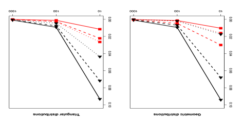
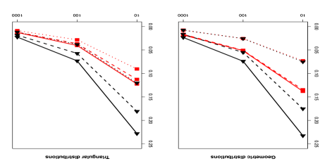
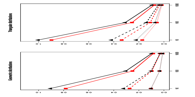
and likewise for $\widetilde{p}_{n}$. The expected $\ell_{2}$-loss is estimated by the mean calculated on the basis of $1000$ simulations and the results are displayed in Figure 1.

As expected from Theorem 2, the constrained estimator $\widehat{p}_{n}$ outperforms the empirical estimator in all configurations in terms of $\ell_{2}$-loss. The difference is larger in the triangular case because of the existence of a region where $p_{0}$ is linear. The empirical estimator $\widetilde{p}_{n}$ gets better and closer to $\widehat{p}_{n}$ as the true distribution $p_{0}$ becomes more convex, i.e., for $\gamma=.9$ or $j=2$. Note that the fit of the unconstrained estimator improves when the true distribution gets more convex.

These results are theoretically grounded by Theorem 2 for the $\ell_{2}$-loss, but we also considered the Kolomogorov loss:

$$K(\widehat{p},p_{0})=\sup_{i}|\widehat{P}_{n}(i)-P_{0}(i)|,$$

where $P_{0}$ is the true cumulative distribution function (cdf) and $\widehat{P}_{n}$ is the constrained cdf. The Kolmogorov loss of the empirical cdf $\widetilde{P}_{n}$ was calculated in the same way. As shown on Figure 1 (bottom), the behavior of the Kolmogorov loss is similar to that of the $\ell_{2}$-loss. The same behavior was observed for the Hellinger loss:

$$\frac{1}{2}\sum_{i}\left(\sqrt{\widehat{p}_{n}(i)}-\sqrt{p_{0}(i)}\right)^{2}$$

and the total variation loss:

$$\frac{1}{2}\sum_{i}|\widehat{p}_{n}(i)-p_{0}(i)|.$$

(results not shown). We thus observed that the constrained estimator $\widehat{p}_{n}$ outperforms the empirical estimator for all considered losses.

Figure 1: $\ell_{2}$-loss. Empirical risk as a function of the sample size $n$. Top: $\ell_{2}(\cdot,p_{0})$, bottom: $K(\cdot,p_{0})$. Black: $\widetilde{p}_{n}$, red: $\widehat{p}_{n}$. Solid (–): $\gamma=1$ or $j=20$, dashed (- -): $\gamma=.5$ or $j=5$, dotted ($\cdots$): $\gamma=.9$ or $j=2$.

4.3 Some characteristics of interest

In this section, we consider the estimation of some characteristics of the distribution, namely the variance, the entropy and the probability at $0$. For each of these characteristics, denoted $\theta(p)$, we measured the performance in terms of relative standard error:

$${\sqrt{\mathbb{E}\left(\theta(\widehat{p}_{n})-\theta(p_{0})\right)^{2}}}\left/{\theta(p_{0})}\right..$$

The expectation was estimated by the mean over 1,000 simulations.

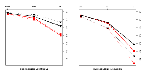
As shown in Section 2, the means of the empirical and constrained distributions are equal, whereas the variance of the constrained distribution is larger than the variance of the empirical one. Denoting by $\mu_{k}$ the centered moment of order $k$ of $p_{0}$, the mean and variance of the empirical variance are respectively

$$\frac{n-1}{n}\mu_{2}\qquad\text{and}\qquad\frac{n-1}{n^{3}}\left((n-1)\mu_{4}-(n-3)\mu_{2}^{2}\right).$$

Figure 2 shows that the relative standard error of the constrained estimator is smaller than that of the empirical one. Hence, the constrained variance turns out to be more accurate.

Figure 2: Variance. Relative standard error of the variance as a function of the sample size $n$. Same legend as Figure 1.

We also investigated the estimation of the entropy

$$H(p)=-\sum_{i\geqslant 0}p(i)\log p(i),$$

which is often used in ecology as a diversity index. As shown in Figure 3, $H(\widehat{p}_{n})$ is a better estimate of the true entropy than $H(\widetilde{p}_{n})$, in most situations; the difference between the two estimators vanishes when the true distribution becomes more convex. The worst performance of $H(\widehat{p}_{n})$ are obtained when the true distribution is $T_{2}$. Note that this distribution is a special case since more than half of the estimation errors consist in adding a component $T_{j}$ ($j>2$) in the mixture (7), which result in an increase of the entropy.

Figure 3: Entropy. Relative standard error of the estimated entropy estimators as a function of the sample size $n$. Same legend as Figure 1.

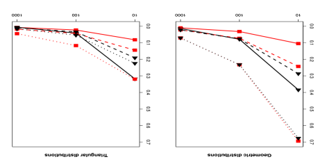
We then considered the estimation of the probability mass $p(0)$. Theorem 3 showed that the constrained estimator $\widehat{p}_{n}(0)$ is greater than or equal to the empirical estimator $\widetilde{p}_{n}(0)$, which is known to be unbiased. However, Figure 4 shows that the constrained estimator $\widehat{p}_{n}$ still provides a more accurate estimate of $p_{0}(0)$ than $\widetilde{p}_{n}$.

Figure 4: Probability mass in 0. Relative standard error of the estimated probability mass in zero as a function of the sample size $n$. Same legend as Figure 1.

For all these characteristics, the constrained distribution provides better estimates than the empirical distribution, provided that the true distribution is indeed convex.

4.4 Robustness to non-convexity

We finally studied the robustness of the constrained estimator to non-convexity. As an example, we considered the Poisson distribution with mean $\lambda$, which is convex as long as $\lambda$ is smaller that $\lambda^{*}=2-\sqrt{2}\simeq.59$. We studied how $\widetilde{p}_{n}$ and $\widehat{p}_{n}$ behave, in terms of $\ell_{2}$-loss, when $\lambda$ exceeds $\lambda^{*}$.

Figure 5: Left: Three different Poisson distributions. Solid (–):$\lambda=\lambda^{*}$, dashed (- -):$\lambda=.8$, dotted ($\cdots$):$\lambda=1$. Right: empirical $\ell_{2}$-loss as a function of $n$. Black: $\widetilde{p}_{n}$, red: $\widehat{p}_{n}$.

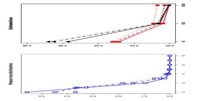
The left panel of Figure 5 displays the Poisson distributions with respective means $\lambda^{*}$, .8 and 1. Figure 5 (right) shows that the $\ell_{2}$-loss of the constrained estimator increases with $\lambda$. However for small sample sizes, $\widehat{p}_{n}$ still provides a better fit than $\widetilde{p}_{n}$, at least for $\lambda\leqslant 1$. The performance of $\widehat{p}_{n}$ is dramatically altered when the sample size becomes large and the convexity assumption is strongly violated.

5 Proofs

5.1 Proof of Theorem 1

In order to prove Theorem 1, we first prove in the following lemma that the minimizer of $Q_{n}$ over ${\cal K}$ exists and is unique, where ${\cal K}$ is the set defined in Section 1. Then, after some intermediate results, we prove in Lemma 3 below that the minimizer of $Q_{n}$ over ${\cal K}$ belongs to ${\cal C}$. Since ${\cal C}\subset{\cal K},$ Theorem 1 follows from Lemma 1 combined to Lemma 3.

Notation

We denote by $N_{n}$ the number of distinct values of the $X_{i}$’s and by $X_{(1)},\dots,X_{(N_{n})}$ these distinct values rearranged in increasing order, i.e., such that $X_{(1)}<\dots<X_{(N_{n})}$. We set $\widetilde{r}_{n}=X_{(1)}$ and $\widetilde{s}_{n}=X_{(N_{n})}$.

In the case $\widetilde{s}_{n}=0$ i.e., $\widetilde{p}_{n}(0)=1$ and $\widetilde{p}_{n}(i)=0$ for all $i\geqslant 1$, the proof of Theorem 1 is straightforward. Thus, in the sequel, we restrict ourselves to the case $\widetilde{s}_{n}\geqslant 1$.

Lemma 1

There exists a unique $\widehat{p}_{n}\in{\cal K}$ such that

$$Q_{n}(\widehat{p}_{n})=\inf_{p\in{\cal K}}Q_{n}(p).$$ (11)

Moreover, $\widehat{p}_{n}$ has a finite support.

Proof.

For proving the existence and uniqueness of $\widehat{p}_{n}$, we have to prove the following preliminary results, where $q$ denotes a candidate to be a minimizer of $Q_{n}$ over ${\cal K}$.

• There exists $c_{1}=c_{1}(\omega)<\infty$ that does not depend on $q$ such that $q\leqslant c_{1}$.

• We have $q=\bar{q}$ where

  $$\bar{q}(i)=\begin{cases}q(i)&\text{ for all }i\in\{0,\dots,\widetilde{s}_{n}\}\\ \max\{q(\widetilde{s}_{n})+(q(\widetilde{s}_{n})-q(\widetilde{s}_{n}-1))(i-\widetilde{s}_{n})\,,\,0\}&\text{ for all }i\geqslant\widetilde{s}_{n}.\end{cases}$$ (12)

Therefore, minimizing $Q_{n}$ over ${\cal K}$ amounts to minimizing $Q_{n}$ over the set of functions $q\in{\cal K}$ such that $q\leqslant c_{1}$, $Q_{n}(q)\leqslant Q_{n}(T_{1})$, and $q=\bar{q}$. But for all $q\in{\cal K}$ such that $q=\bar{q}$, we have

$$Q_{n}(q)=\frac{1}{2}\sum_{i=0}^{\widetilde{s}_{n}}q^{2}(i)+\frac{1}{2}\sum_{i\geqslant 1}\left(\max\{q(\widetilde{s}_{n})+i(q(\widetilde{s}_{n})-q(\widetilde{s}_{n}-1),0\}\right)^{2}-\sum_{i\geqslant 0}q(i)\widetilde{p}_{n}(i)$$ (13)

and therefore, this amounts to minimizing

$$\bar{Q}_{n}(t)=\frac{1}{2}\sum_{i=0}^{\widetilde{s}_{n}}t^{2}(i)+\frac{1}{2}\sum_{i\geqslant 1}\left(\max\{t(\widetilde{s}_{n})+i(t(\widetilde{s}_{n})-t(\widetilde{s}_{n}-1),0\}\right)^{2}-\sum_{i\geqslant 0}t(i)\widetilde{p}_{n}(i)$$

over the set $K$ of non-increasing convex functions $t:\{0,\dots,\widetilde{s}_{n}\}\to[0,\infty)$ such that $t(0)\leqslant c_{1}$ and $\bar{Q}_{n}(t)\leqslant Q_{n}(T_{1})$. The set $K$ is compact and $\bar{Q}_{n}$ is continuous and strictly convex on $K$, so there exists a unique minimizer of $\bar{Q}_{n}$ over $K$. This proves that there exists a unique minimizer of $Q_{n}$ over ${\cal K}$.

It remains to prove results (i) and (ii).

Proof of (i).

It is easy to see that for all $p\in{\cal K}$,

$$Q_{n}(p)\geqslant\frac{1}{2}p^{2}(\widetilde{r}_{n})-p(\widetilde{r}_{n})$$

using that $p$ is non-increasing. This lower bound tends to infinity as $p(\widetilde{r}_{n})\to\infty$. But, if we consider $T_{1}$ the measure that puts the mass 1 in 0, we have $Q_{n}(q)\leqslant Q_{n}(T_{1})<\infty$, so there exists $c<\infty$ such that $q(\widetilde{r}_{n})<c$. Now, $Q_{n}(T_{1})\geqslant Q_{n}(q)\geqslant q^{2}(0)/2-q(\widetilde{r}_{n})$ and therefore, there exists $c_{1}<\infty$ such that $q(0)\leqslant c_{1}$, which means that $q\leqslant c_{1}$.

Proof of (ii).

By convexity we must have $\bar{q}(i)\leqslant q(i)$ for all $i\geqslant\widetilde{s}_{n}$ and therefore,

$$Q_{n}(q)-Q_{n}(\bar{q})=\sum_{i>\widetilde{s}_{n}}(q^{2}(i)-\bar{q}^{2}(i))/2\geqslant 0$$

with a strict inequality in the case $q\neq\bar{q}$. This proves that any candidate $q$ to be a minimizer of $Q_{n}$ over ${\cal K}$ should satisfy $q=\bar{q}$.

Let us now prove that the support of $\widehat{p}_{n}$ is finite. In the case $\widehat{p}_{n}(\widetilde{s}_{n})=0$, it is clear that $\widehat{p}_{n}$ has a finite support included in $\{0,\dots,\widetilde{s}_{n}-1\}$. Consider the case $\widehat{p}_{n}(\widetilde{s}_{n})>0$. Let us first remark that $\widehat{p}_{n}(\widetilde{s}_{n}-1)>\widehat{p}_{n}(\widetilde{s}_{n})$, since otherwise, we would have $\widehat{p}_{n}(i)=\widehat{p}_{n}(\widetilde{s}_{n})$ for all $i\geqslant\widetilde{s}_{n}$ so that $Q_{n}(\widehat{p}_{n})=\infty$. Then define $\bar{q}$ as in (12) where $q$ is replaced by $\widehat{p}_{n}$. From the proof of Lemma 1, we know that $\widehat{p}_{n}=\bar{q}$ which has finite support as soon as $\widehat{p}_{n}(\widetilde{s}_{n}-1)>\widehat{p}_{n}(\widetilde{s}_{n})$. $\Box$

 

The following lemma provides a precise characterization of $\widehat{p}_{n}$. It is the counterpart, in the discrete case, of Lemma 2.2 in Groeneboom et al. (2001) for the continuous case. For every $p\in{\cal K},$ we define

$$F_{p}(j)=\sum_{i=0}^{j}p(i)\text{ and }H_{p}(j)=\sum_{i=0}^{j}F_{p}(i)$$ (14)

for all integers $j\geqslant 0$, and $F_{p}(j)=H_{p}(j)=0$ for all integers $j<0$. Thus, $F_{p}$ is a distribution function in the case $p\in{\cal C}$.

Lemma 2

Let $\widehat{p}_{n}$ be the unique function in ${\cal K}$ that satisfies (11). For all $l\geqslant 1$ we have

$$H_{\widehat{p}_{n}}(l-1)\geqslant H_{\widetilde{p}_{n}}(l-1)$$ (15)

with an equality if $\widehat{p}_{n}$ has a change of slope at point $l$, i.e., if

$$\widehat{p}_{n}(l)-\widehat{p}_{n}(l-1)<\widehat{p}_{n}(l+1)-\widehat{p}_{n}(l).$$

Conversely, if $p\in{\cal K}$ satisfies $H_{p}(l-1)\geqslant H_{\widetilde{p}_{n}}(l-1)$ for all $l\geqslant 1$ with an equality if $p(l)-p(l-1)<p(l+1)-p(l)$, then $p=\widehat{p}_{n}$.

Proof.

First, note that $\widetilde{p}_{n}$ has a finite support by definition, and Lemma 4 ensures that $\widehat{p}_{n}$ has a finite support as well. Thus, all the sums involved in the proof are well-defined and finite. For every $\varepsilon>0$ and $l\geqslant 1$, define $q_{\varepsilon l}$ by $q_{\varepsilon l}(i)=\widehat{p}_{n}(i)$ for all $i\geqslant l$ and

$$q_{\varepsilon l}(i)=\widehat{p}_{n}(i)+\varepsilon(l-i)$$

for all $i\in\{0,\dots,l\}$. Thus, $q_{\varepsilon l}$ is the sum of convex functions, which implies that $q_{\varepsilon l}\in{\cal K}$ for all $\varepsilon,l$. Since $\widehat{p}_{n}$ minimizes $Q_{n}$ over ${\cal K}$, we have $Q_{n}(q_{\varepsilon l})\geqslant Q_{n}(\widehat{p}_{n})$ for all $\varepsilon,l$ and therefore,

$$\liminf_{\varepsilon\downarrow 0}\frac{1}{\varepsilon}\big{(}Q_{n}(q_{\varepsilon l})-Q_{n}(\widehat{p}_{n})\big{)}\geqslant 0$$

for all $l\geqslant 1$. This simplifies to

$$\sum_{i=0}^{l-1}\widehat{p}_{n}(i)(l-i)\geqslant\sum_{i=0}^{l-1}\widetilde{p}_{n}(i)(l-i)$$

for all $l\geqslant 1$ and can be rewritten as

$$\sum_{j=0}^{l-1}\sum_{i=0}^{j}\widehat{p}_{n}(i)\geqslant\sum_{j=0}^{l-1}\sum_{i=1}^{j}\widetilde{p}_{n}(i)$$

for all $l\geqslant 1$, which is precisely (15). To prove the equality case, note that $(1+\varepsilon)\widehat{p}_{n}\in{\cal K}$ for all $\varepsilon>-1$. Therefore, for all $\varepsilon>-1$ we have

$$Q_{n}\big{(}(1+\varepsilon)\widehat{p}_{n}\big{)}\geqslant Q_{n}(\widehat{p}_{n}).$$

Distinguishing the cases $\varepsilon>0$ and $\varepsilon<0$ we obtain

$$\liminf_{\varepsilon\downarrow 0}\frac{1}{\varepsilon}\big{(}Q_{n}((1+\varepsilon)\widehat{p}_{n})-Q_{n}(\widehat{p}_{n})\big{)}\geqslant 0$$

and

$$\limsup_{\varepsilon\uparrow 0}\frac{1}{\varepsilon}\big{(}Q_{n}((1+\varepsilon)\widehat{p}_{n})-Q_{n}(\widehat{p}_{n})\big{)}\leqslant 0.$$

Both limits are equal, so their common value is equal to zero, which can be written as

$$\sum_{i\geqslant 0}\widehat{p}_{n}(i)\big{(}\widehat{p}_{n}(i)-\widetilde{p}_{n}(i)\big{)}=0.$$

Now, noticing that $p(i)=F_{p}(i)-F_{p}(i-1)$ for all $p\in{\cal K}$ and $i\in\mathbb{N}$, we arrive at

$$\begin{split}0=&\sum_{i\geqslant 0}\widehat{p}_{n}(i)\Big{(}F_{\widehat{p}_{n}}(i)-F_{\widehat{p}_{n}}(i-1)-F_{\widetilde{p}_{n}}(i)+F_{\widetilde{p}_{n}}(i-1)\Big{)}\\ =&\sum_{i\geqslant 0}\widehat{p}_{n}(i)\Big{(}F_{\widehat{p}_{n}}(i)-F_{\widetilde{p}_{n}}(i)\Big{)}-\sum_{i\geqslant 1}\widehat{p}_{n}(i)\Big{(}F_{\widehat{p}_{n}}(i-1)-F_{\widetilde{p}_{n}}(i-1)\Big{)}.\\ \end{split}$$

Rearranging the indices, we have

$$\sum_{i\geqslant 1}\widehat{p}_{n}(i)\Big{(}F_{\widehat{p}_{n}}(i-1)-F_{\widetilde{p}_{n}}(i-1)\Big{)}=\sum_{i\geqslant 0}\widehat{p}_{n}(i+1)\Big{(}F_{\widehat{p}_{n}}(i)-F_{\widetilde{p}_{n}}(i)\Big{)},$$

whence

$$0=\sum_{i\geqslant 0}\Big{(}\widehat{p}_{n}(i)-\widehat{p}_{n}(i+1)\Big{)}\Big{(}F_{\widehat{p}_{n}}(i)-F_{\widetilde{p}_{n}}(i)\Big{)}.$$

Now, we notice that $F_{p}(i)=H_{p}(i)-H_{p}(i-1)$ for all $p\in{\cal K}$ and $i\in\mathbb{N}$. A similar change of indices as above then yields

$$0=\sum_{i\geqslant 0}\Big{(}(\widehat{p}_{n}(i)-\widehat{p}_{n}(i+1))-(\widehat{p}_{n}(i+1)-\widehat{p}_{n}(i+2))\Big{)}\Big{(}H_{\widehat{p}_{n}}(i)-H_{\widetilde{p}_{n}}(i)\Big{)}.$$

It follows from (15) that $H_{\widehat{p}_{n}}(i)\geqslant H_{\widetilde{p}_{n}}(i)$ for all $i\geqslant 0$, and we have

$$\widehat{p}_{n}(i+1)-\widehat{p}_{n}(i)\leqslant\widehat{p}_{n}(i+2)-\widehat{p}_{n}(i+1)$$

by convexity of $\widehat{p}_{n}$. A sum of non-negative numbers is equal to zero if and only if these numbers are all equal to zero, so we conclude that

$$\Big{(}(\widehat{p}_{n}(i)-\widehat{p}_{n}(i+1))-(\widehat{p}_{n}(i+1)-\widehat{p}_{n}(i+2))\Big{)}\Big{(}H_{\widehat{p}_{n}}(i)-H_{\widetilde{p}_{n}}(i)\Big{)}=0$$

for all $i\geqslant 0$. Hence, $H_{\widehat{p}_{n}}(i)=H_{\widetilde{p}_{n}}(i)$ for all $i\geqslant 0$ that satisfy

$$\widehat{p}_{n}(i+1)-\widehat{p}_{n}(i)<\widehat{p}_{n}(i+2)-\widehat{p}_{n}(i+1).$$

Setting $l=i+1$, this means that we have an equality in (15) if $\widehat{p}_{n}$ has a change of slope at point $l$.

Conversely, consider $p\in{\cal K}$ such that $H_{p}(i)\geqslant H_{\widetilde{p}_{n}}(i)$ for all $i\geqslant 0$ with an equality if $p(i+1)-p(i)<p(i+2)-p(i+1)$. Then we have

$$0=\sum_{i\geqslant 0}\big{(}p(i)-2p(i+1)+p(i+2)\big{)}\big{(}H_{p}(i)-H_{\widetilde{p}_{n}}(i)\big{)}$$ (16)

and $p$ has a finite support. To see this, argue by contradiction and assume for a while that the support of $p$ is not finite. In such a case, there exists an increasing sequence $(u_{l})_{l\in\mathbb{N}}$ such that $u_{l}$ tends to infinity as $l\to\infty$ and $p$ has changes of slope at every point $u_{l}+1$, $l\in\mathbb{N}$. This implies that

$$H_{p}(u_{l})-H_{p}(u_{l-1})=H_{\widetilde{p}_{n}}(u_{l})-H_{\widetilde{p}_{n}}(u_{l-1})$$

for all $l\geqslant 1$. Using that $F_{p}$ is non-increasing and that $\widetilde{p}_{n}$ has a finite support, we obtain

$$F_{p}(u_{l-1})\leqslant\frac{1}{u_{l}-u_{l-1}}\left(H_{p}(u_{l})-H_{p}(u_{l-1})\right)=F_{\widetilde{p}_{n}}(u_{l})=\sum_{i\geqslant 0}\widetilde{p}_{n}(i)$$

for all large enough $l$ and similarly,

$$F_{p}(u_{l})\geqslant\sum_{i\geqslant 0}\widetilde{p}_{n}(i)$$

for all large enough $l$. Therefore,

$$F_{p}(u_{l})=F_{p}(u_{l-1})=\sum_{i\geqslant 0}\widetilde{p}_{n}(i)$$

for all large enough $l$, which means that $p(i)=0$ for all large enough $i$. This is in contradiction with the assumption that the support of $p$ is not finite, which proves that the support of $p$ is finite.

Now, let $q\in{\cal K}$ be any candidate to be a minimizer of $Q_{n}$ over ${\cal K}$. We know, see the proof of Lemma 1, that $Q_{n}(q)\leqslant Q_{n}(T_{1})$, and $q=\bar{q}$, where $\bar{q}$ is defined by (12). In particular, $q$ satisfies (13) which implies that $q$ has a finite support. Thus, we can write

$$Q_{n}(q)-Q_{n}(p) = \frac{1}{2}\sum_{i\geqslant 0}\Big{(}q^{2}(i)-p^{2}(i)-2\widetilde{p}_{n}(i)\big{(}q(i)-p(i)\big{)}\Big{)}$$ (17)

$$= \frac{1}{2}\sum_{i\geqslant 0}\Big{(}q^{2}(i)-p^{2}(i)+2\big{(}p(i)-\widetilde{p}_{n}(i)\big{)}\big{(}q(i)-p(i)\big{)}-2p(i)\big{(}q(i)-p(i)\big{)}\Big{)}$$

$$= \frac{1}{2}\sum_{i\geqslant 0}\big{(}q(i)-p(i)\big{)}^{2}+\sum_{i\geqslant 0}\big{(}p(i)-\widetilde{p}_{n}(i)\big{)}\big{(}q(i)-p(i)\big{)}$$

$$\geqslant \sum_{i\geqslant 0}\big{(}p(i)-\widetilde{p}_{n}(i)\big{)}\big{(}q(i)-p(i)\big{)}.$$

Using that both $q$ and $p-\widetilde{p}_{n}$ have a finite support and rearranging the indices as above, we show that

$$\begin{split}\sum_{i\geqslant 0}&\big{(}p(i)-\widetilde{p}_{n}(i)\big{)}\big{(}q(i)-p(i)\big{)}\\ &=\sum_{i\geqslant 0}\Big{(}\big{(}q(i)-p(i)\big{)}-2\big{(}q(i+1)-p(i+1)\big{)}+\big{(}q(i+2)-p(i+2)\big{)}\Big{)}\big{(}H_{p}(i)-H_{\widetilde{p}_{n}}(i)\big{)}.\end{split}$$

Combining this with (16) and (17) yields

$$Q_{n}(q)-Q_{n}(p)\geqslant\sum_{i\geqslant 0}\big{(}q(i)-2q(i+1)+q(i+2)\big{)}\big{(}H_{p}(i)-H_{\widetilde{p}_{n}}(i)\big{)}.$$

The right-hand side is non-negative since $H_{p}(i)\geqslant H_{\widetilde{p}_{n}}(i)$ for all $i\geqslant 0$ and $q$ is convex over $\mathbb{N}$, so we conclude that $Q_{n}(q)\geqslant Q_{n}(p)$ for all candidates $q\in{\cal K}$. This means that $p$ minimizes $Q_{n}$ over ${\cal K}$. $\Box$

We are now in a position to prove that $\widehat{p}_{n}$ is a probability mass function, i.e., $\widehat{p}_{n}\in{\cal C}.$

Lemma 3

Let $\widehat{p}_{n}$ be the unique function in ${\cal K}$ that satisfies (11). We have

$$F_{\widetilde{p}_{n}}(\widehat{s}_{n}+1)=F_{\widehat{p}_{n}}(\widehat{s}_{n}+1),$$ (18)

$\widehat{s}_{n}\geqslant\widetilde{s}_{n}$ and $\widehat{p}_{n}\in{\cal C}.$

Proof.

Let us first prove by contradiction that $\widehat{s}_{n}$ is well-defined. Let $k=1+\min_{j}\left\{\widetilde{p}_{n}(j)\neq 0\right\}$. It is easy to verify that there exists a strictly positive $a$ such that $Q_{n}(aT_{k})<0$. As $Q_{n}(0)=0$, $\widehat{p}_{n}$ cannot be identically zero and $\widehat{s}_{n}$ is well-defined.

By definition of $\widehat{s}_{n}$, $\widehat{p}_{n}$ has a change of slope at point $\widehat{s}_{n}+1$, so it follows from Lemma 2 that

$$\sum_{j=0}^{\widehat{s}_{n}}F_{\widehat{p}_{n}}(j)=\sum_{j=0}^{\widehat{s}_{n}}F_{\widetilde{p}_{n}}(j).$$ (19)

Using Lemma 2 again we obtain

$$\sum_{j=0}^{\widehat{s}_{n}+1}F_{\widehat{p}_{n}}(j)\geqslant\sum_{j=0}^{\widehat{s}_{n}+1}F_{\widetilde{p}_{n}}(j),$$

which, combined with (19) shows that $F_{\widehat{p}_{n}}(\widehat{s}_{n}+1)\geqslant F_{\widetilde{p}_{n}}(\widehat{s}_{n}+1)$.

Let us first consider the case where $\widehat{s}_{n}\geqslant 1$. We have

$$\sum_{j=0}^{\widehat{s}_{n}-1}F_{\widehat{p}_{n}}(j)\geqslant\sum_{j=0}^{\widehat{s}_{n}-1}F_{\widetilde{p}_{n}}(j)$$

which, combined with (19) shows that $F_{\widehat{p}_{n}}(\widehat{s}_{n})\leqslant F_{\widetilde{p}_{n}}(\widehat{s}_{n})$. But $\widehat{p}_{n}(\widehat{s}_{n}+1)=0$ by definition of $\widehat{s}_{n}$, so we also have $F_{\widehat{p}_{n}}(\widehat{s}_{n}+1)=F_{\widehat{p}_{n}}(\widehat{s}_{n})$ and therefore,

$$F_{\widetilde{p}_{n}}(\widehat{s}_{n})\geqslant F_{\widehat{p}_{n}}(\widehat{s}_{n}+1)\geqslant F_{\widetilde{p}_{n}}(\widehat{s}_{n}+1).$$

By definition, $F_{\widetilde{p}_{n}}$ is non-decreasing, so we conclude that (18) holds.

Consider now the case $\widehat{s}_{n}=0$. We have $\widetilde{p}_{n}(1)=0$: otherwise, we could modify $\widehat{p}_{n}$ to a $q\in{\cal K}$ such that $q(0)=\widehat{p}_{n}(0)$, $0<q(1)\leqslant\widetilde{p}_{n}(1)$ and $q(i)=0$ for all $i>1$, which is a contradiction since for such a $q$ we have $Q_{n}(q)<Q_{n}(\widehat{p}_{n})$. Moreover, in the case $\widehat{s}_{n}=0$, we have $\widehat{p}_{n}(0)=\widetilde{p}_{n}(0)$: otherwise, we could modify $\widehat{p}_{n}$ to a $q\in{\cal K}$ such that $q(0)=\widetilde{p}_{n}(0)$ and $q(i)=0$ for all $i>0$ which is a contradiction since for such a $q$ we have $Q_{n}(q)<Q_{n}(\widehat{p}_{n})$. Hence,

$$F_{\widehat{p}_{n}}(1)=\widehat{p}_{n}(0)=\widetilde{p}_{n}(0)=F_{\widetilde{p}_{n}}(1),$$

which completes the proof of (18).

For the purpose of proving that $\widehat{s}_{n}\geqslant\widetilde{s}_{n}$, we argue by contradiction. Assume for a while that $\widehat{s}_{n}=\widetilde{s}_{n}-1$. This means that $\widehat{p}_{n}(i)=0$ for all $i\geqslant\widetilde{s}_{n}$ and $\widehat{p}_{n}(\widetilde{s}_{n}-1)>0$. In this case, we can modify $\widehat{p}_{n}$ to a $q\in{\cal K}$ such that $q(i)=\widehat{p}_{n}(i)$ for all $i<\widetilde{s}_{n}$, $0<q(\widetilde{s}_{n})\leqslant\widetilde{p}_{n}(\widetilde{s}_{n}),$ and $q(i)=0$ for all $i>\widetilde{s}_{n}$. Then we have

$$2\big{(}Q_{n}(q)-Q_{n}(\widehat{p}_{n})\big{)} = \sum_{i\geqslant 0}\big{(}q(i)-\widetilde{p}_{n}(i)\big{)}^{2}-\sum_{i\geqslant 0}\big{(}\widehat{p}_{n}(i)-\widetilde{p}_{n}(i)\big{)}^{2}$$

$$= \big{(}q(\widetilde{s}_{n})-\widetilde{p}_{n}(\widetilde{s}_{n})\big{)}^{2}-\big{(}\widetilde{p}_{n}(\widetilde{s}_{n})\big{)}^{2}$$

$$< 0.$$

This is a contradiction since $\widehat{p}_{n}$ minimizes $Q_{n}$ and therefore, $\widehat{s}_{n}\neq\widetilde{s}_{n}-1.$ Assume now that $\widehat{s}_{n}<\widetilde{s}_{n}-1$. Then, $F_{\widetilde{p}_{n}}(\widehat{s}_{n}+1)<1$, so (18) yields

$$F_{\widehat{p}_{n}}(j)=F_{\widehat{p}_{n}}(\widehat{s}_{n}+1)<1$$

for all $j\geqslant\widehat{s}_{n}+1$. Therefore, for all $l>\widetilde{s}_{n}$ we have

$$\sum_{j=0}^{l-1}\big{(}F_{\widehat{p}_{n}}(j)-F_{\widetilde{p}_{n}}(j)\big{)}=\sum_{j=0}^{\widetilde{s}_{n}-1}\big{(}F_{\widehat{p}_{n}}(j)-F_{\widetilde{p}_{n}}(j)\big{)}+(l-\widetilde{s}_{n})\big{(}F_{\widehat{p}_{n}}(\widehat{s}_{n}+1)-1\big{)},$$

which tends to $-\infty$ as $l\to\infty$. This is a contradiction since from Lemma 2, this has to remain non-negative for all $l$. We conclude that $\widehat{s}_{n}\geqslant\widetilde{s}_{n}$. Combining this with (18) yields

$$F_{\widehat{p}_{n}}(\widehat{s}_{n}+1)=F_{\widetilde{p}_{n}}(\widehat{s}_{n}+1)=1.$$

This proves that $\widehat{p}_{n}$ is a probability mass function and completes the proof of the lemma. $\Box$

5.2 Proof of Theorem 2

Let us begin with the following lemma that gathers together a number of properties of the minimizer $\widehat{p}_{n}$. These properties compare to those of the constrained least squares estimator of a convex density function over $[0,\infty)$, see Groeneboom et al. (2001): in this case the constrained LSE has a bounded support, is piecewise linear, has no changes of slope at the observation points, and has at most one change of slope between two consecutive observation points. In the discrete case, the constrained LSE is also piecewise linear with bounded support. However, due to the fact that $\mathbb{N}$ is a discrete set, the constrained LSE can have changes of slopes at the observation points and can have two changes of slopes between two consecutive observations.

Lemma 4

The unique function $\widehat{p}_{n}\in{\cal K}$ that satisfies (11) has the following properties: $\widehat{p}_{n}$ is linear on the interval $\{0,\dots,X_{(1)}+1\}$ and also on $\{\widetilde{s}_{n}-1,\dots,\widehat{s}_{n}\}$; in the case where $N_{n}$, the number of distinct values of the $X_{i}$’s, is greater or equal to 2, it has at most two changes of slopes on $\{X_{(j)},\dots,X_{(j+1)}\}$ for any given $j=1,\dots,N_{n}-1$, and in the case where it has two changes of slopes on this set, these changes occur at consecutive points in $\mathbb{N}$.

Proof.

We know, from the proof of Lemma 1, that $\widehat{p}_{n}=\bar{q}$, where $\bar{q}$ is defined as in (12) where $q$ is replaced by $\widehat{p}_{n}$. It follows that $\widehat{p}_{n}$ is linear on $\{\widetilde{s}_{n}-1,\dots,\widehat{s}_{n}\}$ in the case $\widehat{s}_{n}\geqslant\widetilde{s}_{n}$. Consider an arbitrary candidate $p$ to be a minimizer of $Q_{n}$ over ${\cal K}$, fix $j\in\{1,\dots,N_{n}-1\}$, and define the functions $p_{l}$ and $p_{r}$ over $\mathbb{N}$ as follows: $p_{l}(i)=p(i)$ for all $i\leqslant X_{(j)}+1$ and all $i\geqslant X_{(j+1)}$ and $p_{l}$ is linear over $\{X_{(j)},...,X_{(j+1)}-1\}$, whereas $p_{r}(i)=p(i)$ for all $i\leqslant X_{(j)}$ and all $i\geqslant X_{(j+1)}-1$ and $p_{r}$ is linear over $\{X_{(j)}+1,...,X_{(j+1)}\}$. Setting $q(i)=\max\{p_{l}(i),p_{r}(i)\}$ for all $i\in\mathbb{N}$, we obtain that $q\in{\cal K}$ is piecewise linear over $\{X_{(j)},...,X_{(j+1)}\}$ with at most two changes of slopes over this interval and in case it has two changes of slopes, these changes occur at consecutive points. We have $q(X_{(j)})=p(X_{(j)})$ for all $j$, and $q\leqslant p$ by convexity of $p$. Since $\widetilde{p}_{n}(i)>0$ if and only if $i=X_{(j)}$ for some $j$, this implies that $Q_{n}(q)\leqslant Q_{n}(p)$ with a strict inequality if $p\neq q$. Therefore, $p$ could be a minimizer of $Q_{n}$ only if $p=q$. This implies that the minimizer $\widehat{p}_{n}$ is piecewise linear over $\{X_{(j)},\dots,X_{(j+1)}\}$ with at most two changes of slopes over this interval. A similar argument shows that $\widehat{p}_{n}$ is linear over the interval $\{0,\dots,X_{(1)}+1\}$. $\Box$

Proof of Equation (3)

We prove that (3) holds with $p_{0}$ replaced by any $q\in{\mathcal{K}}$ that belongs to $l_{2}$, i.e., that satisfies $\sum_{j\geqslant 0}q^{2}(j)<\infty$. Since $p_{0}$ belongs to $l_{1}$ as a probability mass function and $l_{2}\subset l_{1}$, $p_{0}$ also belongs to $l_{2}$, so (3) with $p_{0}$ replaced by any $q\in{\mathcal{K}}$ that belongs to $l_{2}$ is a slightly more general result than (3).

Consider an arbitrary $q\in{\mathcal{K}}$ satisfying $\sum_{j\geqslant 0}q^{2}(j)<\infty$. We have

$$\sum_{j\geqslant 0}\big{(}q(j)-\widetilde{p}_{n}(j)\big{)}^{2}\geqslant\sum_{j\geqslant 0}\big{(}q(j)-\widehat{p}_{n}(j)\big{)}^{2}+2\sum_{j\geqslant 0}\big{(}\widehat{p}_{n}(j)-\widetilde{p}_{n}(j)\big{)}\big{(}q(j)-\widehat{p}_{n}(j)\big{)}$$

with a strict inequality in the case where $\widetilde{p}_{n}$ is non-convex since in that case, $\widetilde{p}_{n}\neq\widehat{p}_{n}$. Thus, in order to prove that (3) holds with $p_{0}$ replaced by $q$, it suffices to prove that

$$\sum_{j\geqslant 0}\big{(}\widehat{p}_{n}(j)-\widetilde{p}_{n}(j)\big{)}\big{(}q(j)-\widehat{p}_{n}(j)\big{)}\geqslant 0.$$ (20)

According to Lemma 4, there exist integers $c_{0}<\dots<c_{m}$ such that $c_{0}=0$, $c_{m}=\widehat{s}_{n}+1$, $\widehat{p}_{n}$ is linear over the interval $\{c_{i-1},\dots,c_{i}\}$ and has a change of slope at point $c_{i}$, for all $i=1,\dots,m$. It follows from Theorem 1 that $\widehat{s}_{n}\geqslant\widetilde{s}_{n}$, so $\widetilde{p}_{n}(j)=\widehat{p}_{n}(j)=0$ for all $j\geqslant\widehat{s}_{n}+1$ and the sum in (20) can be split as follows:

$$\sum_{j\geqslant 0}\big{(}\widehat{p}_{n}(j)-\widetilde{p}_{n}(j)\big{)}\big{(}q(j)-\widehat{p}_{n}(j)\big{)}=\sum_{i=1}^{m}\sum_{j=c_{i-1}}^{c_{i}-1}\big{(}\widehat{p}_{n}(j)-\widetilde{p}_{n}(j)\big{)}f(j)$$ (21)

where $f(j)=q(j)-\widehat{p}_{n}(j)$ for all $j\geqslant 0$. For all $i=1,\dots,m$ we have

$$\begin{split}\sum_{j=c_{i-1}}^{c_{i}-1}&\big{(}\widehat{p}_{n}(j)-\widetilde{p}_{n}(j)\big{)}f(j)\\ &=\sum_{j=c_{i-1}}^{c_{i}-1}\left[\big{(}F_{\widehat{p}_{n}}(j)-F_{\widetilde{p}_{n}}(j)\big{)}-\big{(}F_{\widehat{p}_{n}}(j-1)-F_{\widetilde{p}_{n}}(j-1)\big{)}\right]f(j)\\ &=\sum_{j=c_{i-1}}^{c_{i}-1}\big{(}F_{\widehat{p}_{n}}(j)-F_{\widetilde{p}_{n}}(j)\big{)}f(j)-\sum_{j=c_{i-1}-1}^{c_{i}-2}\big{(}F_{\widehat{p}_{n}}(j)-F_{\widetilde{p}_{n}}(j)\big{)}f(j+1)\\ &=\sum_{j=c_{i-1}}^{c_{i}-1}\big{(}F_{\widehat{p}_{n}}(j)-F_{\widetilde{p}_{n}}(j)\big{)}\left(f(j)-f(j+1)\right)\\ &\quad+\big{(}F_{\widehat{p}_{n}}(c_{i}-1)-F_{\widetilde{p}_{n}}(c_{i}-1)\big{)}f(c_{i})\\ &\quad\quad-\big{(}F_{\widehat{p}_{n}}(c_{i-1}-1)-F_{\widetilde{p}_{n}}(c_{i-1}-1)\big{)}f(c_{i-1}),\end{split}$$

where $F_{\widehat{p}_{n}}$ and $F_{\widetilde{p}_{n}}$ are defined in (14). By definition, $F_{\widetilde{p}_{n}}(j)=F_{\widehat{p}_{n}}(j)=0$ for all $j<c_{0}$, so summing up over $i$ yields

$$\sum_{i=1}^{m}\sum_{j=c_{i-1}}^{c_{i}-1}\big{(}\widehat{p}_{n}(j)-\widetilde{p}_{n}(j)\big{)}f(j) = \sum_{i=1}^{m}\sum_{j=c_{i-1}}^{c_{i}-1}\big{(}F_{\widehat{p}_{n}}(j)-F_{\widetilde{p}_{n}}(j)\big{)}\left(f(j)-f(j+1)\right)$$

$$+\big{(}F_{\widehat{p}_{n}}(c_{m}-1)-F_{\widetilde{p}_{n}}(c_{m}-1)\big{)}f(c_{m}),$$

where we recall that $c_{m}=\widehat{s}_{n}+1$. Now, it follows from the definition of $\widehat{s}_{n}$ that $\widehat{p}_{n}(\widehat{s}_{n}+1)=0$ and we also have $\widetilde{p}_{n}(\widehat{s}_{n}+1)=0$ since $\widehat{s}_{n}\geqslant\widetilde{s}_{n}$, see Theorem 1. Thanks to (18), we conclude that $F_{\widetilde{p}_{n}}(\widehat{s}_{n})=F_{\widehat{p}_{n}}(\widehat{s}_{n})$. Therefore, (21) combined with the preceding display yields

$$\begin{split}\sum_{j\geqslant 0}&\big{(}\widehat{p}_{n}(j)-\widetilde{p}_{n}(j)\big{)}\big{(}q(j)-\widehat{p}_{n}(j)\big{)}\\ &=\sum_{i=1}^{m}\sum_{j=c_{i-1}}^{c_{i}-1}\big{(}F_{\widehat{p}_{n}}(j)-F_{\widetilde{p}_{n}}(j)\big{)}\left(f(j)-f(j+1)\right).\end{split}$$

Now, $H_{\widetilde{p}_{n}}(j)=H_{\widehat{p}_{n}}(j)=0$ for all $j<c_{0}$ and $F_{p}(j)=H_{p}(j)-H_{p}(j-1)$ for $p=\widetilde{p}_{n},\widehat{p}_{n}$ and all $j$, so we can repeat the same arguments as above to obtain

$$\begin{split}\sum_{i=1}^{m}&\sum_{j=c_{i-1}}^{c_{i}-1}\big{(}F_{\widehat{p}_{n}}(j)-F_{\widetilde{p}_{n}}(j)\big{)}\left(f(j)-f(j+1)\right)\\ &=\sum_{i=1}^{m}\sum_{j=c_{i-1}}^{c_{i}-1}\big{(}H_{\widehat{p}_{n}}(j)-H_{\widetilde{p}_{n}}(j)\big{)}\left(f(j)-2f(j+1)+f(j+2)\right)\\ &\quad+\big{(}H_{\widehat{p}_{n}}(c_{m}-1)-H_{\widetilde{p}_{n}}(c_{m}-1)\big{)}(f(c_{m})-f(c_{m}+1)).\end{split}$$

Since $\widehat{p}_{n}$ has a change of slope at each $c_{i}$, we deduce from Lemma 2 that $H_{\widehat{p}_{n}}(c_{i}-1)=H_{\widetilde{p}_{n}}(c_{i}-1)$ for all $i=1,\dots,m$ and we arrive at

$$\begin{split}\sum_{j\geqslant 0}&\big{(}\widehat{p}_{n}(j)-\widetilde{p}_{n}(j)\big{)}\big{(}q(j)-\widehat{p}_{n}(j)\big{)}\\ &=\sum_{i}\sum_{j=c_{i-1}}^{c_{i}-2}\big{(}H_{\widehat{p}_{n}}(j)-H_{\widetilde{p}_{n}}(j)\big{)}\left(f(j)-2f(j+1)+f(j+2)\right),\end{split}$$ (22)

where the first sum on the right-hand side is taken over those $i=1,\dots,m$ such that $c_{i-1}\leqslant{c_{i}-2}$. For such an $i$, $f$ is convex over the interval $\{c_{i-1},\dots,c_{i}\}$ as a sum of a convex function and a linear function (recall that by definition of the $c_{i}$’s, $\widehat{p}_{n}$ is linear over such an interval). Therefore we get

$$f(j)-2f(j+1)+f(j+2)\geqslant 0$$

for all $j=c_{i-1},\dots,c_{i}-2$, see (2). Moreover, it follows from Lemma 2 that $H_{\widehat{p}_{n}}\geqslant H_{\widetilde{p}_{n}}$, which leads to

$$\big{(}H_{\widehat{p}_{n}}(j)-H_{\widetilde{p}_{n}}(j)\big{)}\left(f(j)-2f(j+1)+f(j+2)\right)\geqslant 0$$

for all $j=c_{i-1},\dots,c_{i}-2$. Combining this with (22) yields (20) and completes the proof of the first part of the theorem.

Proof of Equations (4) and (5)

It suffices to prove (4) since the second assertion follows from (4) and 3. To prove (4), note that

$$\mathbb{P}\Big{(}\widetilde{p}_{n}\text{ is non-convex}\Big{)}\geqslant\mathbb{P}\left(\widetilde{p}_{n}(i)-2\widetilde{p}_{n}(i+1)+\widetilde{p}_{n}(i+2)<0\right)$$

and that by assumption, we have $p_{0}(i)-2p_{0}(i+1)+p_{0}(i+2)=0$. Therefore, we have the following inequality:

$$\begin{split}&\mathbb{P}\Big{(}\widetilde{p}_{n}\text{ is non-convex}\Big{)}\\ &\quad\geqslant\mathbb{P}\left(\sqrt{n}\Big{[}(\widetilde{p}_{n}(i)-p_{0}(i))-2(\widetilde{p}_{n}(i+1)-p_{0}(i+1))+(\widetilde{p}_{n}(i+2)-p_{0}(i+2))\Big{]}<0\right).\end{split}$$

From the central limit theorem, the random variable

$$\sqrt{n}\Big{[}(\widetilde{p}_{n}(i)-p_{0}(i))-2(\widetilde{p}_{n}(i+1)-p_{0}(i+1))+(\widetilde{p}_{n}(i+2)-p_{0}(i+2))\Big{]}$$

converges, as $n\to\infty$, to a centered Gaussian variable $X$ with a non-degenerate variance and therefore,

$$\liminf_{n\to\infty}\mathbb{P}\left(\widetilde{p}_{n}\text{is non-convex}\right)\geqslant\mathbb{P}(X\leqslant 0).$$

The lemma follows since $\mathbb{P}(X\leqslant 0)=1/2$. $\Box$

5.3 Proof of Theorem 3

Let us first note that for any positive concave function $q$ defined on $\mathbb{N}$, such that $q(\widehat{s}_{n})>0$ and $q(i)=0$ for all $i>\widehat{s}_{n}$, the function $\widehat{p}_{n}-\varepsilon q$ belongs to ${\cal K}$ as soon as $\varepsilon\leqslant\widehat{p}_{n}(\widehat{s}_{n})/q(\widehat{s}_{n})$.

Besides, thanks to Theorem 1, we know that $\widehat{p}_{n}=\mbox{ Argmin}_{f\in{\cal K}}Q_{n}(f)$. Therefore for all $q$ defined as above,

$$0 \leqslant \lim_{\varepsilon\searrow 0}\frac{Q_{n}(\widehat{p}_{n}-\varepsilon q)-Q_{n}(\widehat{p}_{n})}{\varepsilon}$$

$$= \sum_{i=0}^{\widehat{s}_{n}}(\widetilde{p}_{n}(i)-\widehat{p}_{n}(i))q(i).$$

Let $u\geqslant 1$, $0\leqslant a\leqslant\widehat{s}_{n}$, and take

$$q(i)=\left(1-\left(\frac{|i-a|}{\widehat{s}_{n}+1-a}\right)^{u}\right),\mbox{ for }1\leqslant i\leqslant\widehat{s}_{n},$$

and $q(i)=0$ for $i>\widehat{s}_{n}$. Then we get the inequality in Equation (6).

The proof of $\sum_{i=1}^{\widetilde{s}_{n}}i\widetilde{p}_{n}(i)=\sum_{i=1}^{\widehat{s}_{n}}i\widehat{p}_{n}(i)$ follows from the fact that the function $\widehat{p}_{n}+\varepsilon q$ belongs to ${\cal K}$ for

$$q(i)=\left(1-\frac{i}{\widehat{s}_{n}+1}\right)\mbox{ for }1\leqslant i\leqslant\widehat{s}_{n},\mbox{ and }q(i)=0,\mbox{ for }i>\widehat{s}_{n}.$$

It remains to prove that $\widehat{p}_{n}(0)\geqslant\widetilde{p}_{n}(0)$. Argue by contradiction and assume that $\widehat{p}_{n}(0)<\widetilde{p}_{n}(0)$. Define $q(0)=\widetilde{p}_{n}(0)$ and $q(i)=\widehat{p}_{n}(i)$ for all $i\geqslant 1$. Then, $q\in{\cal K}$ since $\widehat{p}_{n}$ is convex and $q(0)\geqslant\widehat{p}_{n}(0)$, and we have $Q_{n}(q)<Q_{n}(\widehat{p}_{n})$. This is a contradiction since $\widehat{p}_{n}$ minimizes $Q_{n}$ over ${\cal K}$, see Theorem 1. This completes the proof of the theorem.

5.4 Proof of Theorem 4

Assume $f\in{\cal K}$ and consider the function $\pi$ defined by (8). The function $\pi$ takes non-negative values since $f$ is convex, see (2). Therefore $\pi$ belongs to ${\cal M}$. Moreover, for all $i\in\mathbb{N}$ we have

$$\sum_{j\geqslant i+1}\pi_{j}T_{j}(i) = \sum_{j\geqslant i+1}\big{(}f(j+1)+f(j-1)-2f(j)\big{)}(j-i)$$

$$= \sum_{j\geqslant i+1}\sum_{k=1}^{j-i}\big{(}f(j+1)+f(j-1)-2f(j)\big{)}.$$

Since all terms in the sum are non-negative and $\lim_{i\to\infty}f(i)=0$, we can write

$$\sum_{j\geqslant i+1}\pi_{j}T_{j}(i) = \sum_{k\geqslant 1}\sum_{j\geqslant i+k}\big{(}f(j+1)+f(j-1)-2f(j)\big{)},$$

$$= \sum_{k\geqslant 1}\big{(}f(i+k-1)-f(i+k)\big{)}$$

$$= f(i)$$

for all $i\in\mathbb{N}$. Therefore, $\pi\in{\cal M}$ satisfies (7). Conversely, every $f:\mathbb{N}\to[0,\infty)$ satisfying (7) for some $\pi\in{\cal M}$ is clearly convex, so we obtain the first assertion of the theorem. To prove the second and the third assertions, we assume that $f\in{\cal K}$. So, in view of the preceding result, we know that $f$ satisfies (7) for some $\pi\in{\cal M}$. Thus, we have

$$f(i-1)-f(i) = \sum_{j\geqslant i}\pi_{j}\big{(}T_{j}(i-1)-T_{j}(i)\big{)}$$

$$= \sum_{j\geqslant i}\frac{2\pi_{j}}{j(j+1)}$$

for all $i\geqslant 1$. By convexity of $f$ we conclude that

$$0\leqslant\big{(}f(i-1)-f(i)\big{)}-\big{(}f(i)-f(i+1)\big{)}=\frac{2\pi_{i}}{i(i+1)}$$

for all $i\geqslant 1$, which implies that $\pi$ is uniquely defined by (8). Moreover,

$$\sum_{i\geqslant 0}f(i)=\sum_{i\geqslant 0}\sum_{j\geqslant i+1}\pi_{j}T_{j}(i)=\sum_{i\geqslant 0}\sum_{j\geqslant 1}\pi_{j}T_{j}(i)$$

since $T_{j}(i)=0$ for all $j\leqslant i$. This implies that

$$\sum_{i\geqslant 0}f(i)=\sum_{j\geqslant 1}\pi_{j}\big{(}\sum_{i\geqslant 0}T_{j}(i)\big{)}$$

where $\sum_{i\geqslant 0}T_{j}(i)=1$. This completes the proof of the theorem. $\Box$

5.5 Proof of Theorem 5

The theorem is proved following the work of Groeneboom and al. Groeneboom et al. (2008). It follows from Lemmas 5 and 6 given below.

Lemma 5

Let $\widetilde{s}_{n}$ be the maximum of the support of $\widetilde{p}_{n}$ and $L\geqslant\widetilde{s}_{n}+1$. Then we have the following result: $\widehat{\pi}^{L}=\arg\min_{\mu\in{\mathcal{M}}^{L}}\Psi_{n}(\mu)$ is equivalent to

$$\left[d_{j}(\Psi_{n})\right](\widehat{\pi}^{L})\geqslant 0\;\forall 1\leqslant j\leqslant L,\mbox{ and }\left[d_{j}(\Psi_{n})\right](\widehat{\pi}^{L})=0\;\forall j\in\mbox{Supp}(\widehat{\pi}^{L})$$ (23)

Proof.

Let $\widehat{\pi}^{L}=\arg\min_{\mu\in{\mathcal{M}}^{L}}\Psi_{n}(\mu)$.

For all $1\leqslant j\leqslant L$ and $\varepsilon>0$, $\widehat{\pi}^{L}+\varepsilon\delta_{j}\in{\mathcal{M}}^{L}$, and $\Psi_{n}(\widehat{\pi}^{L}+\varepsilon\delta_{j})\geqslant\Psi_{n}(\widehat{\pi}^{L})$. It follows that $\left[d_{j}(\Psi_{n})\right](\widehat{\pi}^{L})\geqslant 0$.

If $j\in\mbox{Supp}(\widehat{\pi}^{L})$, then for $\varepsilon>0$ small enough, $\widehat{\pi}^{L}-\varepsilon\delta_{j}\in{\mathcal{M}}^{L}$, and $\Psi_{n}(\widehat{\pi}^{L}-\varepsilon\delta_{j})\geqslant\Psi_{n}(\widehat{\pi}^{L})$. It follows that $-\left[d_{j}(\Psi_{n})\right](\widehat{\pi}^{L})\geqslant 0$.

Conversely, assume that Equation (23) is satisfied, and take $\pi\in{\mathcal{M}}^{L}$. Then $\left[D_{\pi}(\Psi_{n})\right](\widehat{\pi}^{L})$ is non negative and $\left[D_{\widehat{\pi}^{L}}(\Psi_{n})\right](\widehat{\pi}^{L})=0$, thanks to Equation (10).

By convexity of $\Psi_{n}$, for $\varepsilon>0$

$$\Psi_{n}(\pi)-\Psi_{n}(\widehat{\pi}^{L})\geqslant\frac{1}{\varepsilon}\left(\Psi_{n}(\varepsilon\pi+(1-\varepsilon)\widehat{\pi}^{L})-\Psi_{n}(\widehat{\pi}^{L})\right).$$

Taking the limit when $\varepsilon$ tends to 0, we get

$$\Psi_{n}(\pi)-\Psi_{n}(\widehat{\pi}^{L}) \geqslant \left[D_{\pi-\widehat{\pi}^{L}}(\Psi_{n})\right](\widehat{\pi}^{L})$$

$$= \left[D_{\pi}(\Psi_{n})\right](\widehat{\pi}^{L})\geqslant 0.$$

$\Box$

Lemma 6

Let us define the following quantities.

• Let $\pi=\sum_{i=1}^{L-1}a_{i}\delta_{j_{i}}$ be the minimizer of $\Psi_{n}$ over the set of positive measures spanned by $\left\{\delta_{j_{i}},\;1\leqslant i\leqslant L-1\right\}$.

• Let $j_{L}$ be an integer such that $j_{L}\neq j_{i}$ for all $i=1,\ldots,L-1$, and $\left[d_{j_{L}}(\Psi_{n})\right](\pi)<0$.

• Let $\pi^{\star}=\sum_{i=1}^{L}b_{i}\delta_{j_{i}}$ be the minimizer of $\Psi_{n}$ over the set spanned by $\left\{\delta_{j_{i}},\;1\leqslant i\leqslant L\right\}$.

Then $b_{L}>0$, and there exists $\varepsilon>0$ such that $\pi+\varepsilon(\pi^{\star}-\pi)$ is a non negative measure, and such that $\Psi_{n}(\pi+\varepsilon(\pi^{\star}-\pi))<\Psi_{n}(\pi)$.

Proof.

Following the same arguments as in the proof of Lemma 5, we have $\left[d_{j_{i}}(\Psi_{n})\right](\pi)=0$ for all $i=1,\ldots,L-1$. Then

$$\left[D_{\pi}(\Psi_{n})\right](\pi)=\sum_{i=1}^{L-1}a_{i}\left[d_{j_{i}}(\Psi_{n})\right](\pi)=0.$$

Moreover, we have

$$\Psi_{n}(\pi+\varepsilon\delta_{j_{L}})=\Psi_{n}(\pi)+\frac{\varepsilon^{2}}{2}+\varepsilon\left[d_{j_{L}}(\Psi_{n})\right](\pi).$$

Therefore, $\left[d_{j_{L}}(\Psi_{n})\right](\pi)<0$ implies that for $\varepsilon>0$ small enough,

$$\Psi_{n}(\pi+\varepsilon\delta_{j_{L}})<\Psi_{n}(\pi).$$

This shows that $\pi^{\star}\neq\pi$.

By convexity of $\Psi_{n}$, we show that

$$\lim_{\varepsilon\downarrow 0}\frac{\Psi_{n}((1-\varepsilon)\pi+\varepsilon\pi^{\star})-\Psi_{n}(\pi)}{\varepsilon} \leqslant \lim_{\varepsilon\downarrow 0}\frac{(1-\varepsilon)\Psi_{n}(\pi)+\varepsilon\Psi_{n}(\pi^{\star})-\Psi_{n}(\pi)}{\varepsilon}$$

$$= \Psi_{n}(\pi^{\star})-\Psi_{n}(\pi)<0.$$

This shows that for $\varepsilon>0$ small enough, $\Psi_{n}(\pi+\varepsilon(\pi^{\star}-\pi))<\Psi_{n}(\pi)$.

Besides, we have

$$\lim_{\varepsilon\downarrow 0}\frac{1}{\varepsilon}\left(\Psi_{n}((1-\varepsilon)\pi+\varepsilon\pi^{\star})-\Psi_{n}(\pi)\right) = \left[D_{\pi^{\star}-\pi}(\Psi_{n})\right](\pi)$$

$$= \left[D_{\pi^{\star}}(\Psi_{n})\right](\pi)$$

$$= \sum_{i=1}^{L}b_{i}\left[d_{j_{i}}(\Psi_{n})\right](\pi)$$

$$= b^{L}\left[d_{j_{L}}(\Psi_{n})\right](\pi).$$

Because $\left[d_{j_{L}}(\Psi_{n})\right](\pi)<0$, $b_{L}$ is positive.

It remains to show that there exists $\varepsilon>0$ such that, for all $1\leqslant i\leqslant L-1$, $a_{i}+\varepsilon(b_{i}-a_{i})$ is non negative. This is clearly the case if $b_{i}\geqslant a_{i}$. If not, take $\varepsilon\leqslant\min_{b_{i}<a_{i}}\left\{a_{i}/(a_{i}-b_{i})\right\}$. $\Box$

5.6 Proof of Theorem 6

Let us begin with the following lemma.

Lemma 7

If $\widehat{\pi}^{L}=\arg\min_{\mu\in{\mathcal{M}}^{L}}\Psi_{n}(\mu)$, then for all $j\geqslant 1$,

$$\left[d_{L+j}(\Psi_{n})\right](\widehat{\pi}^{L})=b\left(\sum_{i=1}^{L}\widehat{\pi}^{L}_{i}-1\right),$$

for some positive constant $b$ depending on $j$ and on the maximum of the support of $\widehat{\pi}^{L}$.

Proof.

Let us consider two cases according to wether $\widehat{\pi}^{L}_{L}$ equals 0 or not.

Suppose that $\widehat{\pi}^{L}_{L}>0$, and write

$$\left[d_{L+j}(\Psi_{n})\right]({\widehat{\pi}}^{L}) = \sum_{l=1}^{L+j-1}T_{L+j}(l)\left(\sum_{j^{\prime}=l+1}^{L}{\widehat{\pi}}^{L}_{j^{\prime}}T_{j^{\prime}}(l)-\widetilde{p}_{n}(l)\right)$$

$$= \sum_{l=1}^{L-1}T_{L+j}(l)\left(\sum_{j^{\prime}=l+1}^{L}\widehat{\pi}^{L}_{j^{\prime}}T_{j^{\prime}}(l)-\widetilde{p}_{n}(l)\right).$$

Because for $0\leqslant l\leqslant L-1$, $T_{L+j}(l)=aT_{L}(l)+b$, for constants $a$ and $b$ depending on $L$ and $j$, we get

$$\left[d_{L+j}(\Psi_{n})\right](\widehat{\pi}^{L})=a\left[d_{L}(\Psi_{n})\right](\widehat{\pi}^{L})+b\left[\sum_{l=1}^{L-1}\sum_{j^{\prime}=l+1}^{L}\widehat{\pi}_{j^{\prime}}^{L}T_{j^{\prime}}(l)-1\right].$$

Following Lemma 5, $\left[d_{L}(\Psi_{n})\right](\widehat{\pi}^{L})=0$, and we get

$$\left[d_{L+j}(\Psi_{n})\right](\widehat{\pi}^{L})=b\left(\sum_{i=1}^{L}\widehat{\pi}^{L}_{i}\sum_{l=0}^{j-1}T_{j}(l)-1\right)=b\left(\sum_{i=1}^{L}\widehat{\pi}^{L}_{i}-1\right).$$

If $\widehat{\pi}^{L}_{L}=0$, then $\widehat{\pi}^{L}\in{\mathcal{M}}^{L_{1}}$ for some $L_{1}<L$. Thanks to Lemma 5, we know that $\widehat{\pi}^{L}$ is the minimizer of $\Psi_{n}$ over ${\mathcal{M}}^{L_{1}}$. Then we can show that $\left[d_{L_{1}+j}(\Psi_{n})\right](\widehat{\pi}^{L})=0$ for all $j\geqslant 1$ exactly as we have done in the case $\widehat{\pi}^{L}_{L}>0$.

 

To conclude the proof of Theorem 6, note first that for all $L^{\prime}\leqslant L$, we have ${\mathcal{M}}^{L^{\prime}}\subset{\mathcal{M}}^{L}$, which implies

$$\Psi_{n}(\widehat{\pi}^{L})\leqslant\Psi_{n}(\widehat{\pi}^{L^{\prime}}).$$ (24)

Second, it follows from Lemmas 5 and 7 that if $\sum_{i=1}^{L}\widehat{\pi}^{L}_{i}=1$, then for all $L^{\prime}\geqslant L$, $\widehat{\pi}^{L^{\prime}}=\widehat{\pi}^{L}$. Therefore Equation (24) holds for all positive integers $L^{\prime}$, which implies that

$$\Psi_{n}(\widehat{\pi}^{L})\leqslant\Psi_{n}(\pi)$$

for all measures $\pi\in\cal M$ with a finite support. Therefore $\widehat{\pi}^{L}=\widehat{\pi}_{n}$. $\Box$

References

- Balabdaoui et al. (2011) Balabdaoui, F., Jankowski, H., Rufibach, K., 2011. Maximum likelihood estimation and confidence bands for a discrete log-concave distribution. ArXiv:1107.3904.
- Balabdaoui and Wellner (2005) Balabdaoui, F., Wellner, J. A., 2005. Mixtures and monotonicity: a review of estimation under monotonicity constraints. IMS Lecture Notes - Monograph Series.
- Barlow et al. (1972) Barlow, R. E., Bartholomew, D. J., Bremmer, J. M., Brunk, H. D., 1972. Statistical Inference under Order Restrictions. New-York : Wiley.
- Böhning et al. (2005) Böhning, D., Dietz, E., Kuhnert, R., Schön, D., 2005. Mixture models for capture-recapture count data. Statis. Meth. Appli. 14, 29–43, dOI: 10.1007/s10260-005-0103-0.
- Böhning and Kuhnert (2006) Böhning, D., Kuhnert, R., Dec 2006. Equivalence of truncated count mixture distributions and mixtures of truncated count distributions. Biometrics 62, 1207–1215.
-
Chao and Shen (2004)
Chao, A., Shen, T.-J., 2004. Nonparametric prediction in species sampling
9 (3), 253–269+.
URL http://dx.doi.org/10.1198/108571104x3262 - Dumbgen et al. (2007) Dumbgen, L., Husler, A., Rufibach, K., 2007. Active set and EM algorithms for log-concave densities based on complete and censored data. Available at http://arxiv.org/abs/0707.4643.
- Groeneboom et al. (2008) Groeneboom, P., Jongbloed, G., Wellner, J., Sep 2008. The Support Reduction Algorithm for Computing Non-Parametric Function Estimates in Mixture Models. Scand Stat Theory Appl 35, 385–399.
- Groeneboom et al. (2001) Groeneboom, P., Jongbloed, G., Wellner, J. A., 2001. Estimation of a convex function: characterizations and asymptotic theory. Ann. Statist. 29, 1653–1698.
- Jankowski and Wellner (2009) Jankowski, H. K., Wellner, J., 2009. Estimation of a discrete monotone distribution. Electron J Stat 3, 1567–1605.
- Rufibach (2006) Rufibach, K., 2006. Log-concave density estimation and bump hunting for i.i.d. observations, PhD Thesis. Universities of Bern and Gottingen.
- Rufibach (2007) Rufibach, K., 2007. Computing maximum likelihood estimators of a log-concave density function. J. Statist. Comput. and Simul. 77, 561–574.