Phase lag in epidemics on a network of cities

Abstract

We study the synchronisation and phase-lag of fluctuations in the number of infected individuals in a network of cities between which individuals commute. The frequency and amplitude of these oscillations is known to be very well captured by the van Kampen system-size expansion, and we use this approximation to compute the complex coherence function that describes their correlation. We find that, if the infection rate differs from city to city and the coupling between them is not too strong, these oscillations are synchronised with a well defined phase lag between cities. The analytic description of the effect is shown to be in good agreement with the results of stochastic simulations for realistic population sizes.

I Introduction

The theory of the frequency and amplitude of stochastic oscillations in models of epidemics of childhood diseases has been extensively developed over the last few years Alonso et al. (2007); Simoes et al. (2008); Rozhnova and Nunes (2009a, b); Black et al. (2009); Rozhnova and Nunes (2010); Black and McKane (2010a, b); Kuske et al. (2007); Ghose and Adhikari (2010), but the question of the synchrony of these oscillations has received comparatively little attention. This is despite its undoubted importance; whether the oscillations in different locations are in phase or out of phase with each other will clearly have consequences for the duration of an epidemic and for the persistence of a disease. The particular case of in-phase and antiphase locking of epidemics in coupled cities has been described and interpreted in the literature Rohani et al. (1999); He and Stone (2003), but only for models that exhibit periodic oscillations in the infinite population limit. Similarly, synchronisation in models of coupled oscillators has been extensively studied Pikovsky et al. (2001), including in particular demographic oscillators Galla , but not in the context of epidemics.

This subject has been so little investigated from a theoretical point of view, that it is useful to recall a simpler, and more familiar example. It is frequently argued in connection with predator-prey interactions that if predator numbers happen to be high, prey numbers will subsequently fall due to increased predation, and when prey numbers fall, predator numbers will subsequently fall due to lack of food. This is actually an argument which relates to fluctuations in the number of predators and prey and would seem to indicate oscillations, with predator and prey numbers being out of phase with each other.

A similar argument, although not so well-known, can be applied to infected and susceptible individuals in a city. In both cases, the frequency and amplitude of these oscillations is very well captured by the van Kampen system-size expansion Alonso et al. (2007); Simoes et al. (2008); Rozhnova and Nunes (2009a, b); Black et al. (2009); Rozhnova and Nunes (2010); Black and McKane (2010a, b); McKane and Newman (2005); van Kampen (2007), and it seems reasonable to suppose that the same approach should also be able to quantify the synchrony and phase-lag between oscillations of different kinds of individuals. In this paper we apply this method to study possible synchronisation between fluctuations in the number of infected individuals in a network of cities between which individuals commute.

A previous study Rozhnova et al. (2011) has shown that if the parameter setting the infection rate, denoted by $\beta$, is the same for all cities in the network, then the stochastic dynamics takes a remarkably simple form. This has been known for some time in the case of the deterministic dynamics: a rather general theorem tells us that in this case the fraction of susceptible, infected and recovered individuals is the same in all cities Guo et al. (2008). In Ref. Rozhnova et al. (2011), it was shown that the stochastic oscillations in this situation are also quite simple, having only one frequency, which is independent of the city, even if the sizes of the cities are different. As we will show later, these oscillations are synchronised between cities, but with no phase lag, in agreement with the findings reported in the literature for stochastic simulations of infection dynamics on coupled population patches Lloyd and May (1996); Rohani et al. (1999). Exploring spatial heterogeneity as a means to overcome some of the shortcomings of the standard description of epidemics, namely in the predicted frequency of disease fade-outs, was one of the goals of these studies. In this sense, the trivial phase relation between cities is a negative result.

However, it was assumed in previous work that the infection rate $\beta$ is the same in all cities. If $\beta$ is taken to be different in different cities, the symmetry of the fixed point is broken, which introduces the possibility of more complex oscillations. There are other ways of achieving this, but within the framework in which we will work, this is a natural way of introducing the symmetry breaking. We shall see that, under these conditions, the numbers of infected individuals fluctuate with a phase lag between cities, provided that the coupling is not too strong.

The paper is structured as follows. In Sec. II we describe the stochastic model, including a microscopic interpretation of the parameters in terms of the mobility patterns of the populations and the characteristics of the disease. The deterministic equations in the infinite population limit are derived in Sec. III, as are the Langevin equations for the fluctuations around the non-trivial deterministic equilibrium in the linear noise approximation, found using van Kampen’s system-size expansion. In Sec. IV we introduce the complex coherence function that measures the cross-correlations between different cities and/or types of individuals, and we compute it for susceptibility and infection in the simple case of one city as an illustration of the method. The correlation between infection in two cities is studied in Sec. V and it is shown that for moderate coupling and different $\beta$ the fluctuations have a characteristic frequency range and phase relation. This is extended to the case of three cities in Sec. VI. We conclude in Sec. VII.

II Model

The model consists of $n$ cities, labeled $j=1,\ldots,n$ containing individuals who are infected, susceptible or recovered from a disease. As is common, for mathematical convenience the total number of individuals in a particular city, $N_{j}$ for city $j$, is fixed. This means that the number of recovered individuals in each city may be expressed in terms of the number of infected and the number of susceptible individuals: $R_{j}=N_{j}-S_{j}-I_{j}$, $j=1,\ldots,n$. This reduces the number of degrees of freedom from three to two per city, considerably simplifying the analysis. It also means that deaths and births are coupled, with the random death of an individual giving rise to the birth of a susceptible individual, and so providing a fresh victim for the disease.

We will have in mind a particular type of interchange of individuals between cities, but we will see that the construction which comes from this is sufficiently general to encompass a large variety of situations. A concrete example of what we have in mind is a set of residential areas and one or more urban areas; there would typically be a significant fraction of commuters from the former to the latter, and fewer from the latter to the former. The model will thus allow for a fraction of the individuals from city $j$ to commute to city $k$, denoted by $f_{kj}$, with the number of non-commuters (residents) in city $j$ being $1-f_{j}\equiv 1-\sum_{k\neq j}f_{kj}$. The model will differ from that studied in Ref. Rozhnova et al. (2011) in that we will take into account the different nature of the city (for instance, residential or urban) by allowing the parameter describing the rate of infection, $\beta$, to vary from city to city.

If we denote the state of the system of $n$ cities at a given time by $\sigma\equiv\{S_{1},I_{1},\ldots,S_{n},I_{n}\}$, then the recovery of an individual in city $j$ will occur at a rate $\gamma I_{j}$ and cause a transition to the new state $\sigma^{\prime}=\{S_{1},I_{1},\ldots,S_{j},I_{j}-1,\ldots,S_{n},I_{n}\}$. We will write the transition rate for this case as

$$T(S_{j},I_{j}-1|S_{j},I_{j})=\gamma I_{j},$$ (1)

with the initial state on the right and the final state on the left. It should be noted that we have only listed only the variables in city $j$ in order to lighten the notation. In a similar fashion, the death of an infected or recovered individual, and the birth of a susceptible, in city $j$ are given by

$$T(S_{j}+1,I_{j}-1|S_{j},I_{j}) = \mu I_{j},$$

$$T(S_{j}+1,I_{j}|S_{j},I_{j}) = \mu(N_{j}-S_{j}-I_{j}),$$ (2)

respectively.

The network structure manifests itself when constructing the transition rates induced by infections. The rate of infections involving susceptibles from city $j$ and infectives from city $k$ will be proportional to $S_{j}I_{k}$. There will be five types of term. In two of them $k=j$. These are when the infective residents in city $j$ infect susceptible residents in city $j$ and when infective commuters from city $j$ infect susceptible commuters from city $j$ in city $\ell$ ($\ell\neq j$). The rates for these are respectively $\beta_{j}(1-f_{j})^{2}S_{j}I_{j}/M_{j}$ and $\beta_{\ell}f^{2}_{\ell j}S_{j}I_{j}/M_{\ell}$, where $\beta_{j}$ is the parameter which characterises the infection rate in city $j$ and where $M_{j}$ is the number of individuals in city $j$:

$$M_{j}=\left(1-f_{j}\right)N_{j}+\sum_{m\neq j}f_{jm}N_{m}.$$ (3)

The other three terms result when the susceptibles from city $j$ are infected by individuals from city $k$ where cities $j$ and $k$ are different. Then, infective commuters can infect resident susceptibles at a rate $\beta_{j}(1-f_{j})f_{jk}S_{j}I_{k}/M_{j}$, infective residents can infect commuting susceptibles at a rate $\beta_{k}f_{kj}(1-f_{k})S_{j}I_{k}/M_{k}$ and finally infective commuters from city $k$ infect susceptible commuters from city $j$ in city $\ell$ ($\ell\neq j,k$) at a rate $\beta_{\ell}f_{\ell j}f_{\ell k}S_{j}I_{k}/M_{\ell}$. These results allow us to write down the transition rate for infection as

$$T(S_{j}-1,I_{j}+1|S_{j},I_{j})=\sum^{n}_{k=1}\beta_{jk}\frac{S_{j}I_{k}}{N_{k}},$$ (4)

where

$$\beta_{jj} = \frac{\beta_{j}\left(1-f_{j}\right)^{2}N_{j}}{M_{j}}+\sum_{\ell\neq j}\frac{\beta_{\ell}f_{\ell j}^{2}N_{j}}{M_{\ell}},\ \ j=1,\ldots,n,$$

$$\beta_{jk} = \frac{\beta_{j}\left(1-f_{j}\right)f_{jk}N_{k}}{M_{j}}+\frac{\beta_{k}f_{kj}\left(1-f_{k}\right)N_{k}}{M_{k}}$$ (5)

$$+ \sum_{\ell\neq j,k}\frac{\beta_{\ell}f_{\ell j}f_{\ell k}N_{k}}{M_{\ell}},\ \ j,k=1,\ldots,n;j\neq k.$$

Although we have a particular picture of how individuals move between cites, and of the assignment of infection rates to the cities themselves, the final form of the transition rate (4) is quite general. Our results will therefore apply to a wide range of the possible types of interchanges of individuals and choice of infection parameters. Unlike the case where the $\beta_{j}$ were all equal Rozhnova et al. (2011), the $\beta_{jk}$ have no relations between them, and so in general are independent. Therefore they can be chosen from a consideration of Eq. (5) or simply externally imposed.

III Dynamics

The model defined in Section II is stochastic and Markovian, since the transition rates (1), (2) and (4) do not depend on past states of the system. This means that adopting a continuous time description, the time evolution of the system may be obtained from a master equation for $P(\sigma,t)$, the probability distribution for finding the system in state $\sigma$ at time $t$ van Kampen (2007); Risken (1989); Gardiner (2009)

$$\frac{dP(\sigma,t)}{dt}=\sum_{\sigma^{\prime}\neq\sigma}\left[T(\sigma|\sigma^{\prime})P(\sigma^{\prime},t)-T(\sigma^{\prime}|\sigma)P(\sigma,t)\right],$$ (6)

where the $T(\sigma|\sigma^{\prime})$ are each of the rates (1), (2) and (4) taken in turn van Kampen (2007); Risken (1989); Gardiner (2009).

The full master equation (6) cannot be solved exactly, but the aspects that concern us here can be analysed in a remarkably precise way using the system-size expansion of van Kampen van Kampen (2007). We have carried out this calculation on a simpler version of this model — when all the $\beta_{j}$ were equal — elsewhere Rozhnova et al. (2011), and while the predictions are different, the method of carrying out the expansion is very similar. A comparison of the transition rates shows that the results for the model we are investigating here may be obtained from those in Ref. Rozhnova et al. (2011) by substituting $\beta c_{jk}$ by $\beta_{jk}$. We will therefore only briefly indicate the steps in the analysis, and refer the reader to Ref. Rozhnova et al. (2011) for more details.

The method begins by making the following ansatz van Kampen (2007):

$$S_{j}=N_{j}s_{j}+N_{j}^{1/2}x_{j},\ \ I_{j}=N_{j}i_{j}+N_{j}^{1/2}y_{j},$$ (7)

where $j=1,\ldots,n$. Here $s_{j}=\lim_{N_{j}\to\infty}S_{j}/N_{j}$ and $i_{j}=\lim_{N_{j}\to\infty}I_{j}/N_{j}$ are the fraction of individuals from city $j$ which are respectively susceptible and infected in the deterministic limit. Therefore the variables are broken down into a sum of deterministic terms, $s_{j}$ and $i_{j}$, and the stochastic deviations from these, $x_{j}$ and $y_{j}$. The deterministic terms satisfy the ordinary differential equations

$$\dfrac{ds_{j}}{dt} = -\sum^{n}_{k=1}\beta_{jk}s_{j}i_{k}+\mu\left(1-s_{j}\right),$$

$$\dfrac{di_{j}}{dt} = \sum^{n}_{k=1}\beta_{jk}s_{j}i_{k}-\left(\gamma+\mu\right)i_{j},$$ (8)

where $j=1,\ldots,n$.

The stochastic fluctuations, $x_{j}$ and $y_{k}$, which describe the linear fluctuations around trajectories of the deterministic set of equations (8), are found to obey a set of linear stochastic differential equations. For convenience we introduce the vector of these fluctuations $\mathbf{z}=(x_{1},\ldots,x_{n},y_{1},\ldots,y_{n})$ and indices $J,K=1,\ldots,2n$, Then these stochastic differential equations have the form van Kampen (2007); Risken (1989); Gardiner (2009)

$$\frac{dz_{J}}{dt}=\sum_{K=1}^{2n}A_{JK}z_{K}+\eta_{J}(t),\ \ J=1,\ldots,2n,$$ (9)

where $\eta_{J}(t)$ are Gaussian noise terms with zero mean which satisfy $\langle\eta_{J}(t)\eta_{K}(t^{\prime})\rangle=B_{JK}\delta(t-t^{\prime})$. The two $2n\times 2n$ matrices $A$ and $B$ are obtained from the expansion procedure. In fact, to determine the matrix $A$ it is not necessary to carry out the full system-size expansion, since it is related to the Jacobian, ${\cal J}$, found from linear stability analysis about a fixed point of Eq. (8). The precise relationship is ${\cal J}=S^{-1}AS$, where $S={\rm diag}(\sqrt{N_{1}},\ldots,\sqrt{N_{n}})$ Rozhnova et al. (2011). The explicit forms for ${\cal J}$ and $B$ are most easily given in terms of the four $n\times n$ submatrices:

$${\cal J}=\left[\begin{array}[]{c|c}{\cal J}^{(1)}&{\cal J}^{(2)}\\ \hline\cr{\cal J}^{(3)}&{\cal J}^{(4)}\end{array}\right],$$ (10)

and similarly for $B$. The elements of these submatrices are found to be

$${\cal J}^{(1)}_{jk} = -\mu\delta_{jk}-\delta_{jk}\sum_{\ell=1}^{n}\beta_{j\ell}i_{\ell},$$

$${\cal J}^{(2)}_{jk} = -s_{j}\beta_{jk},$$

$${\cal J}^{(3)}_{jk} = \delta_{jk}\sum_{\ell=1}^{n}\beta_{j\ell}i_{\ell},$$

$${\cal J}^{(4)}_{jk} = -(\mu+\gamma)\delta_{jk}+s_{j}\beta_{jk},$$ (11)

and

$$B^{(1)}_{jk} = \mu\delta_{jk}\left(1-s_{j}\right)+\delta_{jk}\sum_{\ell=1}^{n}s_{j}\beta_{j\ell}i_{\ell},$$

$$B^{(2)}_{jk}=B^{(3)}_{jk} = -\mu\delta_{jk}i_{j}-\delta_{jk}\sum_{\ell=1}^{n}s_{j}\beta_{j\ell}i_{\ell},$$

$$B^{(4)}_{jk} = \left(\gamma+\mu\right)\delta_{jk}i_{j}+\delta_{jk}\sum_{\ell=1}^{n}s_{j}\beta_{j\ell}i_{\ell}.$$ (12)

These matrices depend on the solutions $s_{j}$ and $i_{j}$ of Eq. (8), and so on time, but since we will be interested in fluctuations about the stationary state, we use the fixed point values of $s_{j}$ and $i_{j}$, denoted as $s^{*}_{j}$ and $i^{*}_{j}$. The resulting matrices, ${\cal J}^{*}$ and $B^{*}$, are then time-independent.

IV Analysis

Adding the two sets of equations in (8), we immediately see that the fixed points satisfy

$$\left(\gamma+\mu\right)i^{*}_{j}=\mu\left(1-s^{*}_{j}\right),\ \ j=1,\ldots,n.$$ (13)

Using this equation to eliminate the $i^{*}$, one finds that

$$s^{*}_{j}\left[\left(\gamma+\mu\right)+\sum^{n}_{k=1}\beta_{jk}\left(1-s^{*}_{k}\right)\right]=\left(\gamma+\mu\right),\ \ j=1,\ldots,n.$$ (14)

We will assume that the matrix of the coupling coefficients $\beta_{jk}$ is irreducible, which means that any two cities have a direct or indirect interaction. Otherwise the $n$ cities may be split into non-interacting subsets, and several equilibria may be found by combining disease extinction in some subsets with non-trivial equilibrium in other subsets. The disease extinction fixed point is simple to find. If we assume that any one of the $i^{*}$ is zero, for instance $i^{*}_{\ell}=0$, then from Eq. (13) $s^{*}_{\ell}=1$. From Eq. (8) we see immediately that $\sum^{n}_{k=1}\beta_{\ell k}i^{*}_{k}=0$. Since the matrix of couplings is irreducible, and from Eq. (5) the entries are non-negative, it follows that $i^{*}_{k}=0$ for all $k$.

Although it is difficult, and in most cases impossible, to determine any non-trivial fixed points analytically, a theorem Guo et al. (2008) tells us that a unique stable fixed point exists and is stable. The linear stochastic deviations from this fixed point satisfy Eq. (9), with $A$ and $B$ being evaluated at the fixed point. To find the dominant frequencies of the stochastic oscillations, and as we shall see also to study synchronisation and phase-lag, we Fourier transform Eq. (9) to obtain

$$\sum^{2n}_{K=1}\left(-i\omega\delta_{JK}-A_{JK}\right)\tilde{z}_{K}(\omega)=\tilde{\eta}_{J}(\omega),\ \ J=1,\ldots,2n,$$ (15)

where the $\tilde{f}$ denotes the Fourier transform of the function $f$. Defining the matrix $-i\omega\delta_{JK}-A_{JK}$ to be $\Phi_{JK}(\omega)$, the solution to Eq. (15) is

$$\tilde{z}_{J}(\omega)=\sum^{2n}_{K=1}\Phi^{-1}_{JK}(\omega)\tilde{\eta}_{K}(\omega).$$ (16)

We now introduce the matrix

$$P_{JK}(\omega) \equiv \langle\tilde{z}_{J}(\omega)\tilde{z}^{*}_{K}(\omega)\rangle$$ (17)

$$= \sum^{2n}_{L=1}\sum^{2n}_{M=1}\Phi^{-1}_{JL}(\omega)B_{LM}\left(\Phi^{{\dagger}}\right)^{-1}_{MK}(\omega),$$

where $*$ now denotes complex conjugation.

In previous studies, where the focus was on finding the frequencies and amplitudes of the stochastic oscillations Alonso et al. (2007); Simoes et al. (2008); Rozhnova and Nunes (2009a, b); Black et al. (2009); Rozhnova and Nunes (2010); Black and McKane (2010a, b); McKane and Newman (2005), only the power spectrum (when $J=K$) was analysed. Here we will also be interested in the cross-correlations between infection in two different cities, and so will also wish to calculate the cross-spectrum (when $J\neq K$). It is frequently convenient to normalise this by the relevant power-spectrum, and instead work with the complex coherence function (CCF) defined by Neiman (1994); Marple (1987); Stoica and Moses (2005)

$$C_{JK}(\omega)\equiv\frac{P_{JK}(\omega)}{\sqrt{P_{JJ}(\omega)P_{KK}(\omega)}}.$$ (18)

The CCF will in general be complex for $J\neq K$, and so typically one calculates its magnitude and phase, that is, the coherence

$$\left|C_{JK}(\omega)\right|=\frac{\left|P_{JK}(\omega)\right|}{\sqrt{P_{JJ}(\omega)P_{KK}(\omega)}},$$ (19)

and the phase spectrum

$$\phi_{JK}(\omega)\equiv\tan^{-1}\left[\frac{{\rm Im}\left(C_{JK}(\omega)\right)}{{\rm Re}\left(C_{JK}(\omega)\right)}\right]=\tan^{-1}\left[\frac{{\rm Im}\left(P_{JK}(\omega)\right)}{{\rm Re}\left(P_{JK}(\omega)\right)}\right].$$ (20)

Figure 1: (Color online) Synchronisation and phase-lag between susceptible and infected individuals in the one-city SIR model. (a) Analytical power spectra of the fluctuations of susceptibles (solid black line), $P_{11}(\omega)$, and of infectives [solid cyan (gray) line], $P_{22}(\omega)$, given by Eq. (17). The dotted vertical line indicates the frequency $\omega_{max}$ at which these spectra attain maxima. (b) Phase spectrum, $\phi_{21}(\omega)$, and (c) coherence, $\left|C_{21}(\omega)\right|$, for the fluctuations of infectives and susceptibles. The solid lines are the analytical results given by Eq. (22) and Eq. (21). The open circles are the results for the same quantities obtained from simulations. Parameters: $N=10^{6}$, $\beta=17(\gamma+\mu)$, $\mu=1/50$ 1/y and $\gamma=365/13$ 1/y. In all panels the dashed vertical lines bound the frequency range where the stochastic amplification is significant.

As an example of using the CCF to understand synchronisation and phase-lag in systems with sustained stochastic cycles, we apply it to the SIR model in a single city. We could also apply it to the predator-prey system discussed earlier, but we already have the required equations for the one-city SIR model in this paper: Eqs. (8)-(14), with the indices omitted and with $\beta_{jk}$ replaced by $\beta$. It should be emphasised that in this example we are looking at the synchronisation and phase-lag between susceptible and infected individuals, whereas in the actual application of the formalism to $n$ cities, the interest is in possible synchronisation and phase-lag between infected individuals in city $j$ and infected individuals in city $k$.

For models such as the one-city SIR and the predator-prey model, Eq. (19) becomes

$$\left|C_{21}(\omega)\right|=\sqrt{\frac{g_{4}\omega^{4}+g_{2}\omega^{2}+g_{0}}{h_{4}\omega^{4}+h_{2}\omega^{2}+h_{0}}},$$ (21)

where the coefficients of the polynomials are sums of products of the $A_{JK}$ and $B_{JK}$, $J,K=1,2$, which can be found from Eqs. (15)-(19), and Eq. (20) becomes simply

$$\phi_{21}(\omega)=\tan^{-1}\left[\frac{k_{1}\omega}{k_{0}+k_{2}\omega^{2}}\right],$$ (22)

where again $k_{0},k_{1}$ and $k_{2}$ are sums of products of the $A_{JK}$ and $B_{JK}$, $J,K=1,2$.

Figure 2: (Color online) Synchronisation and phase-lag between infected individuals in city 1 and infected individuals in city 2 in the two-city SIR model. (a) Power spectra of the fluctuations of infectives in city 1 (solid black line), $P_{33}(\omega)$, and of infectives in city 2 [solid cyan (gray) line], $P_{44}(\omega)$, given by Eq. (17). The dotted vertical lines indicate the frequencies $\omega_{max_{1}}$ and $\omega_{max_{2}}$ at which these spectra attain maxima. The dashed vertical lines bound the frequency range where the stochastic amplification is significant. (b) Parametric plot of the CCF, $C_{43}(\omega)$, in the complex plane. The solid line is the analytical result given by Eq. (18) [the parts of the curve shown in red (dark gray) and in light gray correspond to $1\leq\omega\leq 5$ and $\{0\leq\omega<1\}\cup\{5<\omega\leq 100\}$, respectively] and the open circles are the result for the same quantity obtained from simulations for $0\leq\omega\leq 10$. Parameters: $\beta_{1}=12(\gamma+\mu)$, $\beta_{2}=17(\gamma+\mu)$, $N_{1}=N_{2}=10^{6}$, $f_{12}=0.001$, $f_{21}=0.01$, $\mu=1/50$ 1/y and $\gamma=365/13$ 1/y.

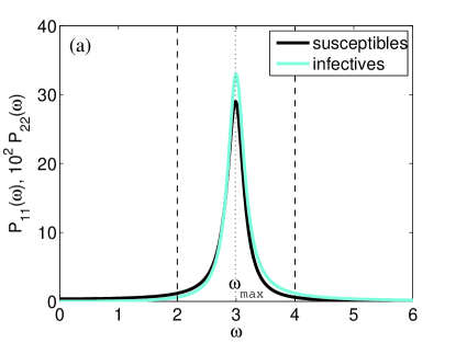
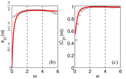
The power spectra of the fluctuations of susceptible and infected individuals computed from Eqs. (17), $P_{11}(\omega)$ and $P_{22}(\omega)$, are shown in Fig. 1 (a). Stochastic amplification gives rise to significant fluctuations in a well-defined frequency range centered at the frequency $\omega_{max}$ where both $P_{11}(\omega)$ and $P_{22}(\omega)$ peak. The coherence, $\left|C_{21}(\omega)\right|$, and phase spectrum, $\phi_{21}(\omega)$, given by Eq. (21) and Eq. (22) are shown in Fig. 1 (c) and (b), respectively, together with the results for the same quantities obtained from numerical simulations. There is very good agreement between the analytic approximation and the simulations in the frequency range where the fluctuations have significant amplitude. Outside of this range, the magnitudes of the power spectra are so low that errors become significant, leading to agreement which is not as good. However within this frequency range the fluctuations of the two kinds of individuals are strongly correlated and have a well-defined phase lag.

The numerical results presented here and in the following sections were obtained from long numerical simulations based on the Gillespie algorithm Gillespie (1976). Each run started from a random initial condition, with the vector of the fluctuations of susceptibles and infectives in $n$ cities, $\mathbf{z}=(x_{1},\ldots,x_{n},y_{1},\ldots,y_{n})$, computed from simulated time series according to Eq. (7), and recorded at equal time intervals. From each simulation run the power and cross spectra for the fluctuations are computed as $\tilde{z}_{J}(\omega)\tilde{z}^{*}_{K}(\omega)$, where $J,K=1,\ldots,2n$ and where $*$ denotes complex conjugation, by using discrete Fourier transforms. The final spectra are averages of $10^{3}$ to $5\times 10^{3}$ simulations. Having computed these, the numerical CCFs, coherence and phase spectra can easily be computed from Eqs. (18)-(20). The values for the epidemiological and demographic parameters used in this paper are those relevant for measles. In all simulations, we take $\mu=1/50$ 1/y and $\gamma=365/13$ 1/y Anderson and May (1991); Keeling and Rohani (2007); Keeling and Grenfell (2002).

V Two cities

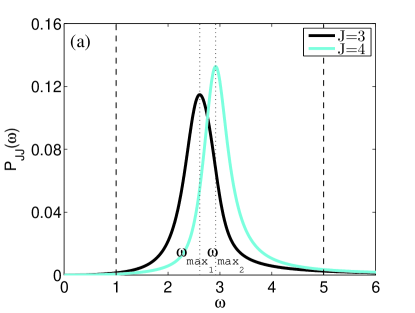
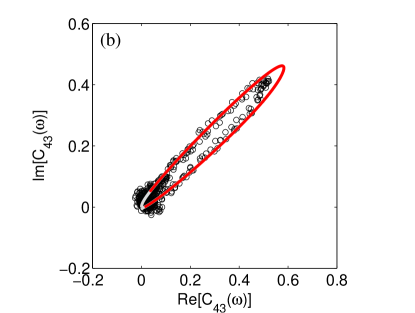
We now turn to the description of the synchronisation and phase-lag between infected individuals in two different cities, using the quantities introduced in Sec. IV. Plots of the power spectra for infectives, $P_{33}(\omega)$ and $P_{44}(\omega)$, are shown in Fig. 2 (a) for a certain choice of parameters (recall that $z_{3}$ and $z_{4}$ are the fluctuations of infection in cities $1$ and $2$ respectively). Different values have been taken for $\beta_{1}$ and $\beta_{2}$, to reflect different social contact patterns in the two cities. In contrast with the spectra for different types of individuals in the one-city case, $P_{33}(\omega)$ and $P_{44}(\omega)$ peak at different frequencies $\omega_{max_{1}}$ and $\omega_{max_{2}}$. The frequency range of interest is bounded by the two dashed vertical lines in the figure — outside this range, $P_{33}$ and $P_{44}$ have negligible amplitude. A parametric plot of the range of the coherence function $C_{43}(\omega)$ in the complex plane is shown in Fig. 2 (b), where the darker (red in the color version) portion of the full line corresponds to the frequency range highlighted in Fig. 2 (a). It can be seen that the fluctuations in the number of those infected in the two cities are correlated and synchronize with a well-defined phase relation in the whole frequency range where both their amplitudes are significant.

Figure 3: Dependence of the synchronisation and phase-lag between infected individuals in city 1 and infected individuals in city 2 on the infection rates in the two-city SIR model. (a) Phase, $\phi_{43}(\omega_{M})$, and (b) coherence, $\left|C_{43}(\omega_{M})\right|$, given by Eq. (20) and by Eq. (19) as a function of $(\beta_{2}-\beta_{1})/(\gamma+\mu)$. (c) The difference between the peak frequencies $\omega_{max_{1}}$ of $P_{33}$ and $\omega_{max_{2}}$ of $P_{44}$ as a function of $(\beta_{2}-\beta_{1})/(\gamma+\mu)$. To obtain the plots $\beta_{2}/(\gamma+\mu)$ was fixed at $15$ and $\beta_{1}/(\gamma+\mu)$ was varied between $5$ and $32.5$. Parameters: $N_{1}=10^{6}$, $N_{2}=2\times 10^{6}$, $f_{12}=0.005$, $f_{21}=0.01$, $\mu=1/50$ 1/y and $\gamma=365/13$ 1/y.

Figure 4: Dependence of the synchronisation and phase-lag between infected individuals in city 1 and infected individuals in city 2 on the fractions of commuters between the cities in the two-city SIR model. The description and coloring are as in Fig. 3. To obtain these log-linear plots, $f_{12}$ was fixed at 0.001 and $f_{21}$ was varied between 0 and 1. Parameters: $\beta_{1}=12(\gamma+\mu)$, $\beta_{2}=17(\gamma+\mu)$, $N_{1}=10^{6}$, $N_{2}=2\times 10^{6}$, $\mu=1/50$ 1/y and $\gamma=365/13$ 1/y.

Also shown in Fig. 2 (b) are the results for $C_{43}(\omega)$ obtained from numerical simulations. There is a good agreement between simulations and analytic results within the frequency resolution limits of the former, showing that for the chosen system sizes the fluctuation cross-correlation behavior is well captured by the linear noise approximation.

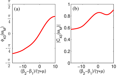
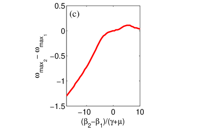
In order to investigate the dependence of the coherence and phase spectrum on the choice of parameters, we have computed the value $\omega_{M}$ for which $\left|C_{43}(\omega)\right|$ attains its maximum, $\left|C_{43}(\omega_{M})\right|$ and $\phi_{43}(\omega_{M})$. A plot of $\phi_{43}(\omega_{M})$ and $\left|C_{43}(\omega_{M})\right|$ as a function of $(\beta_{2}-\beta_{1})/(\gamma+\mu)$ is shown in Fig. 3 (a) and (b). To obtain the plot only the infection rate $\beta_{2}$ was varied while the remaining parameters were kept fixed. With respect to the example of Fig. 2, we have chosen one of the populations, $N_{2}$, to be twice as large and one of the coupling parameters, $f_{12}$, to be five times larger. It should be noted that when $\left(\beta_{2}-\beta_{1}\right)/(\gamma+\mu)$ is so large that the frequency ranges of the stochastic fluctuation peaks in each city no longer overlap, $\left|C_{43}(\omega)\right|$ becomes bimodal instead of unimodal and $\omega_{M}$ is no longer well defined. The difference between the peak frequencies $\omega_{max_{1}}$ of $P_{33}$ and $\omega_{max_{2}}$ of $P_{44}$ is shown in Fig. 3 (c). For values of $\left(\beta_{2}-\beta_{1}\right)/(\gamma+\mu)$ to the left of the represented range, i.e. for values smaller than $-17.5$, this difference becomes larger leading to a more complex synchronization pattern and a bimodal $\left|C_{43}(\omega)\right|$.

We also see that, in this case, fluctuations with a non-trivial phase relation require the two cities to have different values of the infection rates $\beta_{1}$ and $\beta_{2}$. We have found this to be true in general. More precisely, the imaginary parts of the cross spectra of infection $P_{JK}(\omega)$ with $J,K=n+1,\ldots,2n$ and $J\neq K$, as given by Eq. (17), are identically zero when the infection rates $\beta_{i}$, $i=1,\ldots,n$, are the same in all cities, independently of the choice of the population sizes and fractions of commuters. The proof of this result is given in the Appendix. This is compatible with either in-phase or antiphase synchronization.

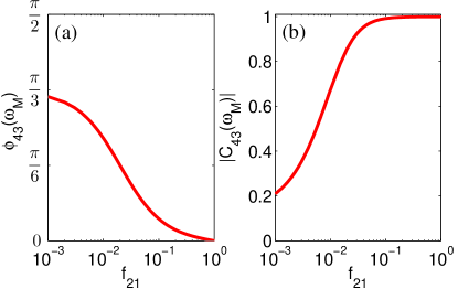
Another condition for $\phi_{43}(\omega_{M})$ to be different from zero is that the coupling between the two cities is not too strong. A plot of $|C_{43}(\omega_{M})|$ and $\phi_{43}(\omega_{M})$ as a function of the coupling $f_{21}$ is shown in Fig. 4. The remaining parameters are as in Fig. 2, except for $N_{2}$, which was taken twice as large. It can be seen that $\left|C_{43}(\omega_{M})\right|$ increases monotonically with $f_{21}$, indicating an increase in cross correlation between infected individuals in the two cities as the coupling gets stronger, but $\phi_{43}(\omega_{M})$ tends to zero with increasing $f_{21}$.

VI Three cities

Figure 5: Synchronisation and phase-lag between infected individuals in three cities with different infection rates in the three-city SIR model. (a) Power spectra of the fluctuations of infectives in city 1, $P_{44}(\omega)$, in city 2, $P_{55}(\omega)$, and in city 3, $P_{66}(\omega)$, given by Eq. (17). The dotted and the dashed vertical lines have the same meanings as in Fig. 2. (b) Parametric plot of the CCFs given by Eq. 18, $C_{54}(\omega)$, $C_{64}(\omega)$, and $C_{65}(\omega)$, in the complex plane. Parameters: $\beta_{1}=7(\gamma+\mu)$, $\beta_{1}\colon\beta_{2}\colon\beta_{3}=7\colon 12\colon 17$, $N_{i}=10^{6}$, $\mu=1/50$ 1/y, $\gamma=365/13$ 1/y, and $f_{ij}=0.005$, where $i=1,2,3$ and $i\neq j$.

Figure 6: An example of synchronisation and phase-lag between infected individuals in three cities in the case when all parameter values are different. The description and coloring are as in Fig. 5. Parameters: $\beta_{1}=7(\gamma+\mu)$, $\beta_{1}\colon\beta_{2}\colon\beta_{3}=7\colon 12\colon 27$, $N_{1}=2\times 10^{6}$, $N_{1}\colon N_{2}\colon N_{3}=2\colon 1\colon 0.5$, $\mu=1/50$ 1/y, $\gamma=365/13$ 1/y, $f_{12}=f_{31}=0.001$, $f_{13}=f_{23}=0.002$, $f_{21}=0.01$, and $f_{32}=0.005$.

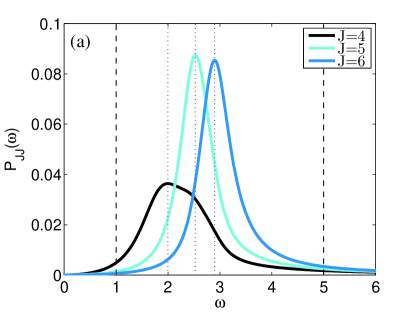
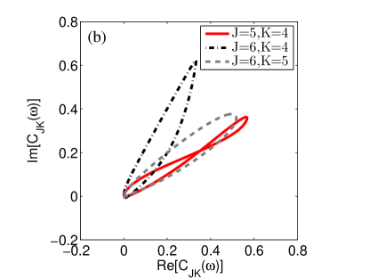
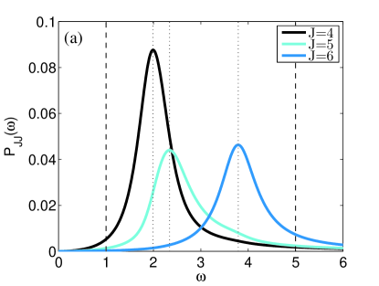
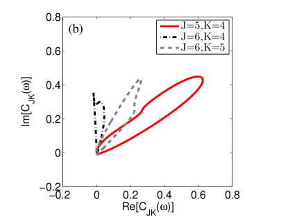
The analysis carried out in Sec. V can be extended to three or more cities. In this Section we will illustrate this by investigating two examples for three cities. We have checked that the approximate analytic description is again in good agreement with the results of simulations, and the plots show the analytic results only, to avoid cluttering.

In the case of Fig. 5, the population sizes are equal, the demographic coupling parameters $f_{ij}$ are all equal, but the three transmission rates $\beta_{j}$, $j=1,2,3$ are different. The power spectra of the fluctuations of infectives in each city, $P_{JJ}$, $J=4,5,6$, shown in Fig. 5 (a), behave as in the example of Fig. 2, as do the coherence and the phase spectra. The ranges of $C_{54}$, $C_{64}$ and $C_{65}$ in the complex plane are plotted in Fig. 5 (b). The phase lags between cities $4$ and $5$ and $5$ and $6$ are approximately the same in this case.

In the example of Fig. 6 we have considered different population sizes and coupling parameters $f_{ij}$ and we have also increased the difference between the transmission rates $\beta_{j}$, $j=1,2,3$ with respect to the previous example. The results for the fluctuation power spectra and for the ranges of $C_{54}$, $C_{64}$ and $C_{65}$ in the complex plane are plotted in Fig. 6 (a) and (b), respectively. In this case we find three different phase lags for the correlated fluctuations in the three city pairs.

These phase lag effects have implications for estimates of the duration of an epidemic and of the likelihood of disease extinction. In a metapopulation model with different transmission rates epidemic bursts should last longer, and disease extinction should occur less frequently than in a single population with the same overall size.

VII Conclusions

In this paper we have considered a stochastic metapopulation version of a susceptible-infected-recovered model representing infection dynamics in different demographically coupled urban centers. We derived the state transition rates of the stochastic process from a microscopic model for the mobility of individuals between cities. Similar rate equations based on a phenomenological coupling parameter have been proposed in the literature. Here we have adopted a bottom-up approach, as an illustration of how the parameters of the general model can be related with the mobility patterns of the sub-populations.

The correlations between the fluctuations in the number of infected in different cities were studied by means of the complex coherence function. It was found that, if the infection rate differed from city to city and the coupling was not too strong, oscillations were observed which were synchronised with a well defined phase lag between cities. We also showed that for realistic population sizes this effect was well described analytically by the linear noise approximation.

The combined effect of stochasticity and demographic coupling as a possible driver of correlations and spatial patterns that are missed by traditional epidemic models was suggested long ago Lloyd and May (1996); Keeling and Rohani (2002). This idea has been left largely unexplored because these early studies based on computer simulations took the infection rate to be the same in different cities. In this case, as we have seen, the fluctuations are trivially synchronized, with no phase lag. However, the infection rate is a phenomenological parameter that depends not only on the disease but also on the rate of potentially infectious contacts that characterize a given social environment. In particular, a strong positive correlation between measles transmission rate and population density was confirmed in recent study based on daily monitoring of urban populations Bharti et al. (2011). The conditions found in this paper for a non-trivial phase relation between the disease incidence fluctuations in connected urban centres can therefore be considered realistic in many settings.

Appendix A Proof that $P^{(4)}$ is real when the infection rates are equal

In this Appendix we will show that the matrix $P_{JK}$ defined by Eq. (17) is real for $J,K=n+1,\ldots,2n$ in the case where the infection rates for each city are equal: $\beta_{j}=\beta$ for all $j$. This shows that the cross-spectra for fluctuations in the number of infected individuals is real, and so that in this case there is either no phase lag or a phase lag of $\pi$. We would expect that the former situation, i.e. no phase lag, would hold, and we have explicitly checked this for the case of two cities. For general $n$ we have a partial proof that the phase lag is zero, and work is underway to complete it.

The results for the situation where $\beta_{j}=\beta$ for all $j$ can be inferred from the results of the current paper, and are given explicitly in Ref. Rozhnova et al. (2011). They are given in terms of the matrices $A$ and $B$ at the fixed point and can be most easily expressed in terms of four $n\times n$ submatrices by writing

$$A=\left[\begin{array}[]{c|c}A^{(1)}&A^{(2)}\\ \hline\cr A^{(3)}&A^{(4)}\end{array}\right],$$ (23)

and similarly for $B$ and $\Phi(\omega)\equiv-i\omega I-A$. Here $I$ is the $n\times n$ identity matrix. The matrices $\Phi^{(1)}$ and $\Phi^{(3)}$ are proportional to the identity matrix and we write them as $\rho I$ and $\sigma I$ respectively. The inverse of $\Phi(\omega)$ then takes the simple form

$$\Phi^{-1}(\omega)=\left[\begin{array}[]{c|c}-\Phi^{(4)}&\Phi^{(2)}\\ \hline\cr\sigma I&-\rho I\end{array}\right]\left[\begin{array}[]{c|c}Y&0\\ \hline\cr 0&Y\end{array}\right],$$ (24)

where $Y^{-1}$ is the $n\times n$ matrix $\sigma\Phi^{(2)}-\rho\Phi^{(4)}$.

In the calculation of $P_{JK}(\omega)$ the matrices $Y$ appear in the combination

$$Z=\left[\begin{array}[]{c|c}Y&0\\ \hline\cr 0&Y\end{array}\right]\left[\begin{array}[]{c|c}B^{(1)}&B^{(2)}\\ \hline\cr B^{(3)}&B^{(4)}\end{array}\right]\left[\begin{array}[]{c|c}Y^{{\dagger}}&0\\ \hline\cr 0&Y^{{\dagger}}\end{array}\right].$$ (25)

However in the case we are interested in Rozhnova et al. (2011), the submatrices $B^{(\alpha)}$, $\alpha=1,\ldots,4$ are diagonal: $B^{(\alpha)}_{jk}\equiv B_{\alpha}\delta_{jk}$ with $j,k=1,\ldots,n$. Therefore

$$Z=\left[\begin{array}[]{c|c}B_{1}YY^{{\dagger}}&B_{2}YY^{{\dagger}}\\ \hline\cr B_{3}YY^{{\dagger}}&B_{4}YY^{{\dagger}}\end{array}\right].$$ (26)

The quantity we wish to study, $P_{JK}(\omega)$, is now given by

$$P=\left[\begin{array}[]{c|c}-\Phi^{(4)}&\Phi^{(2)}\\ \hline\cr\sigma I&-\rho I\end{array}\right]\left[\begin{array}[]{c|c}Z^{(1)}&Z^{(2)}\\ \hline\cr Z^{(3)}&Z^{(4)}\end{array}\right]\left[\begin{array}[]{c|c}-\Phi^{(4){\dagger}}&\bar{\sigma}I\\ \hline\cr\Phi^{(2){\dagger}}&-\bar{\rho}I\end{array}\right],$$ (27)

where $Z^{\alpha}$ is one of the four submatrices given in Eq. (26).

It follows from Eq, (27) that

$$P^{(4)}=\sigma^{2}Z^{(1)}-\sigma\left(\rho+\bar{\rho}\right)Z^{(2)}+|\rho|^{2}Z^{(4)},$$ (28)

where we have used $Z^{(2)}=Z^{(3)}$ which follows from the the symmetry of the matrix $B$ ($B_{2}=B_{3}$), and also used the reality of $\sigma$. We now show that the matrix $Z$ is real, and so that $P^{(4)}$ is real.

To do this we write down the explicit forms for the entries of $\Phi(\omega)$. They are Rozhnova et al. (2011)

$$\rho = \frac{\mu\beta}{\mu+\gamma}-i\omega,$$

$$\sigma = \mu-\frac{\mu\beta}{\mu+\gamma},$$

$$\Phi^{(2)} = \left(\mu+\gamma\right)\chi,$$

$$\Phi^{(4)} = \left(\mu+\gamma-i\omega\right)I-\left(\mu+\gamma\right)\chi,$$ (29)

where $\chi$ is an $n\times n$ matrix given by $\chi_{jk}=\left(N_{j}/N_{k}\right)^{1/2}c_{jk}$, and is real and symmetric (using Eq. (B5) of Rozhnova et al. (2011)). Therefore from the definition of the matrix $Y$

$$Y^{-1}=G(\omega)I+H(\omega)\chi,$$ (30)

with

$$G(\omega)=-\left(\frac{\mu\beta}{\mu+\gamma}-i\omega\right)\left(\mu+\gamma-i\omega\right)$$ (31)

and

$$H(\omega)=\left(\mu+\gamma\right)\left(\mu-i\omega\right).$$ (32)

Using the symmetry and reality of the matrix $\chi$,

$$Y^{-1{\dagger}}Y^{-1} = |G(\omega)|^{2}I+|H(\omega)|^{2}\chi^{2}$$ (33)

$$+ \left\{G(\omega)\overline{H}(\omega)+\overline{G}(\omega)H(\omega)\right\}\chi,$$

which is clearly real. Therefore the inverse of this matrix, $YY^{{\dagger}}$ is also real. From Eq. (26) it follows that $Z$ is real, since $B$ is real.

We end by showing that the cross-spectra for the fluctuations in the number of susceptible individuals is also real in this case. Although we have not explicitly investigated this quantity in the main text, it is also of interest, and by analogy with $P^{(4)}$ we would expect it to be real too. From Eq, (27)

$$P^{(1)} = \Phi^{(4)}Z^{(1)}\Phi^{(4){\dagger}}-\Phi^{(4)}Z^{(2)}\Phi^{(2){\dagger}}$$ (34)

$$- \Phi^{(2)}Z^{(3)}\Phi^{(4){\dagger}}+\Phi^{(2)}Z^{(4)}\Phi^{(2){\dagger}}.$$

Since from Eq. (29), $\Phi^{(4)}=(\mu+\gamma-i\omega)I-\Phi^{(2)}$ and $\Phi^{(2)}$ is real, and since the $Z^{\alpha}$ are real, the imaginary part of $P^{(1)}$ is given by

$${\rm Im}P^{(1)} = \omega\left\{Z^{(1)}\Phi^{(2)}-\Phi^{(2)}Z^{(1)}\right.$$ (35)

$$+ \left.Z^{(2)}\Phi^{(2)}-\Phi^{(2)}Z^{(3)}\right\}.$$

Writing $Z^{\alpha}=B_{\alpha}YY^{{\dagger}}$ and $\Phi^{(2)}=(\mu+\gamma)\chi$ yields

$${\rm Im}P^{(1)}=\omega(\mu+\gamma)\left(B_{1}+B_{2}\right)\left\{\left(YY^{{\dagger}}\right)\chi-\chi\left(YY^{{\dagger}}\right)\right\},$$ (36)

where we have used $B_{3}=B_{2}$. Now from Eq. (33), the matrix $Y^{-1{\dagger}}Y^{-1}$ is a sum of matrices proportional to the identity, $\chi$ and $\chi^{2}$. Therefore it commutes with the matrix $\chi$, that is, $\chi Y^{-1{\dagger}}Y^{-1}=Y^{-1{\dagger}}Y^{-1}\chi$, from which it follows that $YY^{{\dagger}}\chi=\chi YY^{{\dagger}}$, and so from Eq. (36), ${\rm Im}P^{(1)}=0$.

References

- Alonso et al. (2007) D. Alonso, A. J. McKane, and M. Pascual, J. R. Soc. Interface 4, 575 (2007).
- Simoes et al. (2008) M. Simoes, M. M. Telo da Gama, and A. Nunes, J. R. Soc. Interface 5, 555 (2008).
- Rozhnova and Nunes (2009a) G. Rozhnova and A. Nunes, Phys. Rev. E 79, 041922 (2009a).
- Rozhnova and Nunes (2009b) G. Rozhnova and A. Nunes, Phys. Rev. E 80, 051915 (2009b).
- Black et al. (2009) A. J. Black, A. J. McKane, A. Nunes, and A. Parisi, Phys. Rev. E 80, 021922 (2009).
- Rozhnova and Nunes (2010) G. Rozhnova and A. Nunes, Phys. Rev. E 82, 041906 (2010).
- Black and McKane (2010a) A. J. Black and A. J. McKane, J. Theor. Biol. 267, 85 (2010a).
- Black and McKane (2010b) A. J. Black and A. J. McKane, J. R. Soc. Interface 7, 1219 (2010b).
- Kuske et al. (2007) R. Kuske, L. F. Gordillo, and P. E. Greenwood, J. Theor. Biol. 245, 459 (2007).
- Ghose and Adhikari (2010) S. Ghose and R. Adhikari, Phys. Rev. E 82, 021913 (2010).
- Rohani et al. (1999) P. Rohani, D. J. D. Earn, and B. T. Grenfell, Science 286, 968 (1999).
- He and Stone (2003) D. He and L. Stone, Proc. R. Soc. London, Ser. B. 270, 1519 (2003).
- Pikovsky et al. (2001) A. S. Pikovsky, M. G. Rosenblum, and J. Kurths, Synchronization: A Universal Concept in Nonlinear Sciences (Cambridge University Press, Cambridge, 2001).
- (14) T. Galla, arXiv:0811.3689.
- McKane and Newman (2005) A. J. McKane and T. J. Newman, Phys. Rev. Lett. 94, 218102 (2005).
- van Kampen (2007) N. G. van Kampen, Stochastic Processes in Physics and Chemistry (Elsevier, Amsterdam, 2007).
- Rozhnova et al. (2011) G. Rozhnova, A. Nunes, and A. J. McKane, Phys. Rev. E 84, 051919 (2011).
- Guo et al. (2008) H. Guo, M. Y. Li, and Z. Shuai, Proc. Am. Math. Soc. 136, 2793 (2008).
- Lloyd and May (1996) A. L. Lloyd and R. M. May, J. Theor. Biol. 179, 1 (1996).
- Risken (1989) H. Risken, The Fokker-Planck Equation (Springer, Berlin, 1989).
- Gardiner (2009) C. Gardiner, Stochastic Methods: A Handbook for the Natural and Social Sciences (Springer, Berlin, 2009).
- Neiman (1994) A. Neiman, Phys. Rev. E 49, 3484 (1994).
- Marple (1987) S. L. Marple, Digital Spectral Analysis with Applications (Prentice Hall, Upper Saddle River, New Jersey, 1987).
- Stoica and Moses (2005) P. Stoica and R. Moses, Spectral Analysis of Signals (Prentice Hall, Upper Saddle River, New Jersey, 2005).
- Gillespie (1976) D. T. Gillespie, J. Comp. Phys. 22, 403 (1976).
- Anderson and May (1991) R. M. Anderson and R. M. May, Infectious Diseases of Humans: Dynamics and Control (Oxford University Press, Oxford, 1991).
- Keeling and Rohani (2007) M. J. Keeling and P. Rohani, Modelling Infectious Diseases in Humans and Animals (Princeton University Press, Princeton, 2007).
- Keeling and Grenfell (2002) M. J. Keeling and B. T. Grenfell, Proc. R. Soc. London, Ser. B 269, 335 (2002).
- Keeling and Rohani (2002) M. J. Keeling and P. Rohani, Ecol. Lett. 5, 20 (2002).
- Bharti et al. (2011) N. Bharti, A. J. Tatem, M. J. Ferrari, R. F. Grais, A. Djibo, and B. T. Grenfell, Science 334, 1424 (2011).