Precoder Design for Multi-antenna
Partial Decode-and-Forward (PDF)
Cooperative Systems with Statistical CSIT
and MMSE-SIC Receivers

Abstract

Cooperative communication is an important technology in next generation wireless networks. Aside from conventional amplify-and-forward (AF) and decode-and-forward (DF) protocols, the partial decode-and-forward (PDF) protocol is an alternative relaying scheme that is especially promising for scenarios in which the relay node cannot reliably decode the complete source message. However, there are several important issues to be addressed regarding the application of PDF protocols. In this paper, we propose a PDF protocol and MIMO precoder designs at the source and relay nodes. The precoder designs are adapted based on statistical channel state information for correlated MIMO channels, and matched to practical minimum mean-square-error successive interference cancelation (MMSE-SIC) receivers at the relay and destination nodes. We show that under similar system settings, the proposed MIMO precoder design with PDF protocol and MMSE-SIC receivers achieves substantial performance enhancement compared with conventional baselines.

I Introduction

Cooperative communication is an important technology in next generation wireless networks. Exploiting the broadcast nature of wireless transmission, cooperation among different users can be efficiently utilized to significantly increase reliability as well as the achievable rates. In the current literature, various relaying protocols have been proposed taking into consideration of the duplexing constraint [1]. Conventional relaying protocols include amplify-and-forward (AF) and decode-and-forward (DF). For AF protocols, the relay node simply scales and forwards the received signal to the destination node. One disadvantage of AF protocols is the noise amplification in the process of repeating the received signal. On the other hand, for DF protocols, the relay node forwards a clean copy of the decoded source message to the destination node. However, the relay node only assists with data transmission if it can reliably decode the source message, thus resulting in under-utilization of the available resources and performance loss.

To overcome the limitations of conventional AF and DF protocols, various alternative relaying protocols have been proposed in the literature. For example, in [2], the authors proposed a bursty amplify-and-forward (BAF) protocol. It is demonstrated that in the low SNR and low outage probability regime, the achievable $\epsilon$-outage capacity of the BAF protocol is more attractive than conventional AF and DF protocols. In [3], the authors proposed a dynamic decode-and-forward protocol, which is shown to achieve the optimal diversity-multiplexing tradeoff (DMT) when the multiplexing gain is smaller than $1/2$. In [4], the authors proposed a partial decode-and-forward (PDF) protocol for Gaussian broadcast channels. It is assumed that the source node employs a 2-level superposition coding scheme, and the relay node forwards partial information of the source message to the destination node depending on how much information can be decoded. The PDF protocol is especially effective when the relay node cannot reliably decode the complete source message, and can improve upon the relaying efficiency of conventional DF protocols in cooperative relay systems. While a number of works have studied the theoretical capacity of PDF systems, several important practical issues remain to be addressed regarding the application of PDF protocols in multi-antenna cooperative systems.

• Precoder Design for Cooperative PDF Systems: It has been shown that MIMO precoding can effectively boost the performance of multi-antenna cooperative systems [5]. Many prior works considered precoder design at the relay node only (e.g. [6, 7]). In addition, a common assumption is that perfect channel state information (CSI) is available to facilitate precoder design. However, in practice, there may only be imperfect or statistical CSI at the transmitters (CSIT). For instance, in [8], the authors consider relay precoder design in AF relay systems under imperfect CSIT. As we illustrate in this paper, precoder design at both the source and relay nodes is very important to exploit the full benefit of cooperative communication. Furthermore, most existing works on MIMO precoder design for cooperative systems are focused on AF and DF protocols. It is very challenging to design the source and relay node precoders tailoring to the PDF protocol with statistical CSIT.

• Precoder Design Matched to Practical MMSE-SIC Receivers: Precoder design is tightly coupled with the receiver structure at the relay and destination nodes. In [9], the authors consider precoder design for single-stream cooperative system with maximal ratio combining receivers. On the other hand, traditional precoder design for multi-stream cooperative systems assumed either maximum likelihood (ML) receivers [10] or simple linear minimum mean-square-error (LMMSE) receivers [11]. The ML receiver assumption allows for simple precoder design, but ML receivers are difficult to implement in practice and should serve as a performance upper bound. On the other hand, the performance with LMMSE receivers is usually too inferior to the performance with ML receivers. It is well-known that the MMSE successive interference cancelation (MMSE-SIC) receiver is an important practical low-complexity receiver that could bridge the performance gap between ML and LMMSE receivers. While most existing literature consider the power allocation problem to maximize the SINR based system performance [12], very few works have addressed the problem of designing precoders matched to SIC type receivers to enhance system capacity.

In this paper, we propose a MIMO precoder design that is matched to MMSE-SIC receivers for correlated multi-antenna cooperative systems with PDF protocol. Specifically, we consider precoder designs at both the source and relay nodes, given only statistical CSIT, to minimize the average end-to-end per-stream outage probability. We find that under similar system settings, the proposed MIMO precoder design with PDF relay protocol and MMSE-SIC receivers achieves substantial performance enhancement compared with the use of conventional AF and DF relay protocols.

Notations: In the sequel, we adopt the following notations. $\mathbb{C}^{M\times N}$ denotes the set of complex $M\times N$ matrices. Upper and lower case bold letters denote matrices and vectors, respectively. $\textrm{diag}(x_{1},\ldots,x_{N})$ denotes a diagonal matrix with the elements $x_{1},\ldots,x_{N}$ along the diagonal. $\textrm{vec}(\textbf{X})$ denotes the column vector obtained by stacking the columns of X. $[\,\textbf{X}_{1}\,;\,\ldots\,;\,\textbf{X}_{N}\,]$ denotes the matrix obtained by vertically concatenating $\textbf{X}_{1},\ldots,\textbf{X}_{N}$. $[\textbf{X}]_{(a:b,c:d)}$ denotes the $a$-th to the $b$-th row and the $c$-th to the $d$-th column of X. $(\cdot)^{T}$, $(\cdot)^{{\dagger}}$, and $(\cdot)^{\ast}$ denote transpose, Hermitian transpose, and conjugate, respectively. $\det(\cdot)$, $\textrm{Tr}\,(\cdot)$, and $||\cdot||$ denote the determinant, the trace, and the Frobenius norm of a matrix, respectively. $\mathbf{X}\otimes\mathbf{Y}$ denotes the Kronecker product of $\mathbf{X}$ and $\mathbf{Y}$. $\textbf{0}_{M\times N}$ denotes an $M\times N$ matrix of zeros, and $\textbf{I}_{N}$ denotes an $N\times N$ identity matrix. $\mathbb{E}(\cdot)$ denotes expectation. $\textrm{Pr}\,(X|Y)$ denotes the probability of event $X$ given event $Y$.

II System Model

II-A Cooperative Transmission Signal Model

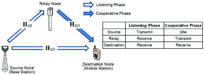
Figure 1: Multi-antenna PDF cooperative system model.

We consider a cooperative system with one source node (a base station), one relay node, and one destination node (a mobile station) as shown in Fig. 1. The source node is equipped with $n_{S}$ antennas, the relay node is equipped with $n_{R}$ antennas, and the destination node is equipped with $n_{D}$ antennas. The source node sends multiple independent data streams to the destination node with the assistance of the relay node, where both the source and relay nodes employ spatial multiplexing transmission. The relay node operates in a half-duplex manner, and data transmission consists of two phases: first, in the listening phase, the source node broadcasts the data to the relay and destination nodes; second, in the cooperative phase, the relay node forwards the source data to the destination node. Each of the listening and cooperative phases lasts for $T$ symbol time slots, and the end-to-end transmission lasts for a transmit time interval (TTI) of $2T$ symbol time slots. We make the following assumptions about the wireless channels.

Assumption 1 (Channel Coherence Properties)

We assume quasi-static frequency flat fading channels, whereby the channel coefficients of all links remain unchanged within each TTI and varies independently from TTI to TTI.  ∎

For each TTI, let $\mathbf{s}^{(1)},\ldots,\mathbf{s}^{(Q)}$ denote the source data streams. Each data stream is separately encoded with an inner space-time block code (STBC) [13, 14, 15] and multiplexed into the data symbols $\mathbf{X}\in\mathbb{C}^{\,n_{\!S}\times T}$. Let $\mathbf{X}_{R}\in\mathbb{C}^{\,n_{\!R}\times T}$ denote the relay node data symbols. The entries of $\mathbf{X}$ and $\mathbf{X}_{R}$ are normalized to have unit average power. Prior to transmission, the source node precodes the data symbols $\mathbf{X}$ using the precoder $\mathbf{P}_{\!S}\in\mathbb{C}^{\,n_{\!S}\times n_{\!S}}$, and the relay node precodes the data symbols $\mathbf{X}_{R}$ using the precoder $\mathbf{P}_{\!R}\in\mathbb{C}^{\,n_{\!R}\times n_{\!R}}$. Let $\mathbf{H}_{SD}\in\mathbb{C}^{\,n_{\!D}\times n_{\!S}}$ denote the channel matrix of the source-destination (SD) link, let $\mathbf{H}_{SR}\in\mathbb{C}^{\,n_{\!R}\times n_{\!S}}$ denote the channel matrix of the source-relay (SR) link, and let $\mathbf{H}_{RD}\in\mathbb{C}^{\,n_{\!D}\times n_{\!R}}$ denote the channel matrix of the relay-destination (RD) link. Accordingly, the received signals of the destination and relay nodes are given by

Listening Phase: $$\mathbf{Y}_{\!D,L}=\mathbf{H}_{SD}\,\mathbf{P}_{\!S}\,\mathbf{X}+\mathbf{Z}_{\!D,L}$$ for the destination node (1a)

Listening Phase: $$\mathbf{Y}_{\!R,L}=\mathbf{H}_{SR}\,\mathbf{P}_{\!S}\,\mathbf{X}+\mathbf{Z}_{\!R,L}$$ for the relay node (1b)

Cooperative Phase: $$\!\!\mathbf{Y}_{\!D,C}=\mathbf{H}_{RD}\,\mathbf{P}_{\!R}\,\mathbf{X}_{R}+\mathbf{Z}_{\!D,C}$$ for the destination node, (2)

where $\mathbf{Z}_{\!D,L},\mathbf{Z}_{\!D,C}\in\mathbb{C}^{\,n_{\!D}\times T}$ and $\mathbf{Z}_{\!R,L}\in\mathbb{C}^{\,n_{\!R}\times T}$ are AWGN with zero mean and variance $N_{0}$. We make the following assumptions about the channel knowledge available at each node.

Assumption 2 (Availability of Channel Knowledge)

• Statistical CSI at the Transmitters: The source node has statistical knowledge of the channel matrices of all links. The relay node has statistical knowledge of the RD link channel matrix.

• Instantaneous CSI at the Receivers: The relay node has knowledge of the precoded channel matrix of the SR link $\mathbf{H}_{SR}\,\mathbf{P}_{\!S}$. The destination node has knowledge of the precoded channel matrices of the SD and RD links $\{\mathbf{H}_{SD}\,\mathbf{P}_{\!S},\mathbf{H}_{RD}\,\mathbf{P}_{\!R}\}$.  ∎

The source and relay nodes derive the precoders $\mathbf{P}_{\!S}$ and $\mathbf{P}_{\!R}$ based on statistical CSI (cf. Section IV). The relay and destination nodes employ MMSE-SIC receivers, where the destination node combines the received signals in the listening and cooperative phases to decode the source data.

Relay Protocol: The form of the relay node data symbols $\mathbf{X}_{R}$ depends on the relay protocol adopted by the cooperative system. Conventional relay protocols can be categorized as AF and DF. For AF protocols, the relay node data symbols are given by the scaled received signals,

$$\textrm{AF: }\mathbf{X}_{R}=\mathbf{Y}_{\!R,L}\mathbf{\Gamma}_{\!R,L},$$ (3)

where $\mathbf{\Gamma}_{\!R,L}\in\mathbb{C}^{\,T\times T}$ is a scaling matrix. In particular, to normalize the entries of $\mathbf{X}_{R}$ to have unit average power, the scaling matrix is given by $\mathbf{\Gamma}_{\!R,L}=\textrm{diag}\Big{(}\frac{n_{\!R}}{||\,[\mathbf{Y}_{\!R,L}]_{(:,1)}||},\ldots,\frac{n_{\!R}}{||\,[\mathbf{Y}_{\!R,L}]_{(:,T)}||}\Big{)}$. For DF protocols, the relay node attempts to decode the source data. If the source data is correctly decoded, the relay node transmits the regenerated data symbols $\widetilde{\mathbf{X}}\in\mathbb{C}^{\,n_{\!R}\times T}$ to the destination node. Conversely, if the source data is incorrectly decoded, the relay node does not transmit. Therefore, the relay node data symbols are given by

$$\textrm{DF: }\mathbf{X}_{R}= \widetilde{\mathbf{X}}\!\!\!\!$$ if the source data is correctly decoded (4a)

$$\textrm{DF: }\mathbf{X}_{R}= \textbf{0}_{n_{\!R}\times T}\!\!\!\!$$ if the source data is incorrectly decoded. (4b)

In Section III-A, we propose a PDF protocol that addresses the deficiencies of the conventional AF and DF protocols.

II-B Correlated MIMO Channel Model

We consider correlated MIMO fading channels that reflect practical communication systems. Specifically, we assume Rayleigh fading with separable correlation properties on the two ends of the link, and the channel matrices can be represented using the Kronecker model.

Definition 1 (Kronecker Model)

The channel matrix $\mathbf{H}\in\mathbb{C}^{M\times N}$ can be represented as $\mathbf{H}=(\mathbf{\Lambda}_{\,r})^{\!1\!\!\>/\!\>2}\mathbf{G}((\mathbf{\Lambda}_{\,t})^{\!1\!\!\>/\!\>2})^{T}$, where $\mathbf{\Lambda}_{\,t}\in\mathbb{C}^{N\times N}$ and $\mathbf{\Lambda}_{\,r}\in\mathbb{C}^{M\times M}$ are the transmit- and receive-side correlation matrices, and $\mathbf{G}\in\mathbb{C}^{M\times N}$ is a random matrix whose entries are independent and identically distributed (i.i.d.) as complex Gaussian with zero mean and unit variance.  ∎

By the Kronecker model, the channel matrices of the different links in the cooperative system can be represented as

$$\mathbf{H}_{SD}=(\mathbf{\Lambda}_{SD,r})^{\!1\!\!\>/\!\>2}\mathbf{G}_{\!SD}((\mathbf{\Lambda}_{SD,t})^{\!1\!\!\>/\!\>2})^{T},\;\mathbf{H}_{SR}=(\mathbf{\Lambda}_{SR,r})^{\!1\!\!\>/\!\>2}\mathbf{G}_{\!SR}((\mathbf{\Lambda}_{SR,t})^{\!1\!\!\>/\!\>2})^{T}$$

$$\mathbf{H}_{RD}=(\mathbf{\Lambda}_{RD,r})^{\!1\!\!\>/\!\>2}\mathbf{G}_{\!RD}((\mathbf{\Lambda}_{RD,t})^{\!1\!\!\>/\!\>2})^{T},$$ (5)

where $\mathbf{\Lambda}_{SD,t}\in\mathbb{C}^{\,n_{\!S}\times\,n_{\!S}}$ and $\mathbf{\Lambda}_{SD,r}\in\mathbb{C}^{\,n_{\!D}\times\,n_{\!D}}$ are the transmit- and receive-side correlation matrices of the SD link, $\mathbf{\Lambda}_{SR,t}\in\mathbb{C}^{\,n_{\!S}\times\,n_{\!S}}$ and $\mathbf{\Lambda}_{SR,r}\in\mathbb{C}^{\,n_{\!R}\times\,n_{\!R}}$ are the transmit- and receive-side correlation matrices of the SR link, and $\mathbf{\Lambda}_{RD,t}\in\mathbb{C}^{\,n_{\!R}\times\,n_{\!R}}$ and $\mathbf{\Lambda}_{RD,r}\in\mathbb{C}^{\,n_{\!D}\times\,n_{\!D}}$ are the transmit- and receive-side correlation matrices of the RD link.

Without loss of generality, we assume that the channel matrices $\{\mathbf{H}_{SD},\mathbf{H}_{SR},\mathbf{H}_{RD}\}$ include the effect of path loss. We discuss a typical operating scenario in the following remark.

Remark 1 (Typical Operating Scenario)

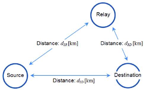
Figure 2: Typical operating scenario. The path loss exponent of the SR link is smaller than those of the SD and RD links. Moreover, the destination node is located closer to the relay node than to the source node. The path loss model for the SR link is given by $-52.4-26\log_{10}(d)~{}\textrm{[dB]}$, the path loss model for the SD and RD links is given by $-52.4-30\log(d)\textrm{[dB]}$, where $d$ is the distance in km between the nodes. The distance of the RD link is smaller than the SD link, so the path loss of the RD link is smaller than the SD link.

In practice, the source node (a base station) and the relay node are mounted on rooftops, whereas the destination node (a mobile station) is at street level. The effect of path loss for the SD link is usually quite severe. Since there is relatively low blockage between the source and relay nodes, the path loss exponent of the SR link is smaller than that of the SD link, and so the SR link is much stronger than the SD link. Moreover, since the destination node always picks a nearby relay node to serve itself, the path loss of the RD link is smaller than that of the SD link, and so the RD link is much stronger than the SD link. We illustrate this typical operating scenario in Fig. 2.  ∎

III Proposed PDF Protocol and Precoder Design Problem Formulation

A number of prior works have focused on theoretical performance characterizations of PDF protocols (e.g. [4]). Instead, in this paper our focus is driven by practical considerations: we propose a PDF protocol and precoder designs that are matched to practical receiver structures, and we characterize the performance of such a system. In the following, we first present the proposed PDF protocol and elaborate its advantages over conventional AF and DF protocols. We then formulate the problem of designing the source and relay node precoders with only statistical CSI at the transmitters. The proposed algorithm is suitable for scenarios in which the relay node cannot reliably decode the complete source message (i.e. when the SR link is not very strong). The PDF protocol and MIMO precoder design lead to a higher probability that the relay node can assist with data transmission and achieve non-uniform diversity protection among spatially multiplexed streams that facilitates successive interference cancelation decoding.

III-A Proposed PDF Protocol

Note that conventional relay protocols have the following key deficiencies.

• For conventional DF protocols, the relay node forwards the source data only if it can correctly decode all the constituent independent data streams. Otherwise, the relay node does not assist with data transmission, thus compromising the achievable cooperative diversity gain.

• With the use of practical MMSE-SIC receivers at the relay and destination nodes (cf. Section II-A), data decoding performance is intricately impacted by the decoding order among the data streams [19]. Specifically, the data streams that are decoded earlier are interfered by the data streams that are decoded subsequently. And yet, decoding errors are propagated over successively decoded data streams. For conventional AF and DF protocols, in the cooperative phase the relay node forwards all (or none) of the source data streams to the destination node. After the destination node combines the received signals in the listening and cooperative phases, all the data streams have the same diversity protection and experience the same order of inter-stream interference. This makes it non-trivial to deduce the decoding order among the data streams that would yield satisfactory overall data decoding performance.

To ameliorate the deficiencies of conventional relay protocols, we propose a PDF protocol whereby the relay node attempts to decode and forward a partial of the source data streams. For notational convenience, we introduce the following definitions.

Definition 2 (Cooperative Streams and Regular Payload Streams)

We define the source data streams that are forwarded by the relay node as the cooperative streams, and define the source data streams that are not forwarded by the relay node as the regular payload streams.  ∎

There is a higher probability that the relay node can correctly decode a partial of the source data streams than it can correctly decode all the data streams. As such, there is a higher probability that the relay node can assist with data transmission based on the proposed PDF protocol than based on conventional DF protocols. Furthermore, after the destination node combines the received signals in the listening and cooperative phases, the cooperative streams that benefit from cooperative spatial diversity have higher diversity protection compared with the regular payload streams. This creates non-uniform diversity protection among the source data streams; the cooperative streams can be reliably decoded first and their interference compensated for, thus the regular payload streams can be decoded free from interference from the cooperative streams.

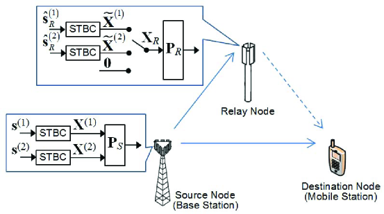
Figure 3: An illustrative example of the proposed PDF protocol. The source node sends two independent data streams to the destination node with the assistance of the relay node. The data streams are space-time block coded and precoded prior to transmission.

For ease of exposition, we present the details of the proposed PDF protocol below focusing on an illustrative scenario where the source node sends two independent data streams to the destination node (cf. Fig. 3).

Processing at the Source Node: Let $\mathbf{s}^{(1)}$ and $\mathbf{s}^{(2)}$ denote the source data streams. Each data stream is separately encoded using STBC: $\mathbf{s}^{(1)}$ is encoded into the symbols $\mathbf{X}^{(1)}\in\mathbb{C}^{\,n_{\!S}^{(1)}\times T}$, $\mathbf{s}^{(2)}$ is encoded into the symbols $\mathbf{X}^{(2)}\in\mathbb{C}^{\,n_{\!S}^{(2)}\times T}$ (where $n_{S}^{(1)}+n_{S}^{(2)}=n_{S}$), and $\mathbf{X}^{(1)}$ and $\mathbf{X}^{(2)}$ are multiplexed into the source node data symbols $\mathbf{X}=[\;\mathbf{X}^{(1)}\,;\mathbf{X}^{(2)}\;]$.

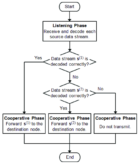
Figure 4: Flow chart of the processing at the relay node. The source node sends two independent data streams to the destination node. The relay node attempts to decode and forward one data stream to the destination node.

Processing at the Relay Node: In the listening phase, the relay node receives the signals $\mathbf{Y}_{\!R,L}$ and attempts to decode one source data stream. In the cooperative phase, the relay node forwards the correctly decoded data stream. The processing at the relay node is illustrated in Fig. 4 and results in three cases.

• PDF Case 1 ($\mathcal{A}_{1}$): In the listening phase, the relay node correctly decodes data stream $\mathbf{s}^{(1)}$. In the cooperative phase, the relay node forwards $\mathbf{s}^{(1)}$ to the destination node.

• PDF Case 2 ($\mathcal{A}_{2}$): In the listening phase, the relay node incorrectly decodes data stream $\mathbf{s}^{(1)}$ but correctly decodes data stream $\mathbf{s}^{(2)}$. In the cooperative phase, the relay node forwards $\mathbf{s}^{(2)}$ to the destination node.

• PDF Case 3 ($\mathcal{A}_{3}$): In the listening phase, the relay node incorrectly decodes both data streams $\mathbf{s}^{(1)}$ and $\mathbf{s}^{(2)}$. In the cooperative phase, the relay node does not transmit.

The cooperative stream is encoded using STBC: when forwarding data stream $\mathbf{s}^{(1)}$ it is encoded into the symbols $\widetilde{\mathbf{X}}^{(1)}\in\mathbb{C}^{\,n_{\!R}\times T}$, and when forwarding data stream $\mathbf{s}^{(2)}$ it is encoded into the symbols $\widetilde{\mathbf{X}}^{(2)}\in\mathbb{C}^{\,n_{\!R}\times T}$. Therefore, the relay node data symbols are given by

$$\textrm{PDF: }\mathbf{X}_{R}= \widetilde{\mathbf{X}}^{(1)}\!\!\!\! \mathbf{s}^{(1)}$$ if is correctly decoded (6a)

$$\textrm{PDF: }\mathbf{X}_{R}= \widetilde{\mathbf{X}}^{(2)}\!\!\!\! \mathbf{s}^{(1)} \mathbf{s}^{(2)}$$ if is incorrectly decoded and is correctly decoded (6b)

$$\textrm{PDF: }\mathbf{X}_{R}= \textbf{0}_{n_{\!R}\times T}\!\!\!\! \mathbf{s}^{(1)} \mathbf{s}^{(2)}$$ if both and are incorrectly decoded. (6c)

Processing at the Destination Node: The destination node combines the received signals in the listening phase $\mathbf{Y}_{\!D,L}$ and the received signals in the cooperative phase $\mathbf{Y}_{\!D,C}$. We first decode the cooperative stream that has higher diversity protection, then after interference cancelation we decode the regular payload stream. For instance, suppose data stream $\mathbf{s}^{(1)}$ is the cooperative stream (i.e. PDF Case 1), we first decode $\mathbf{s}^{(1)}$ and compensate for its interference then decode data stream $\mathbf{s}^{(2)}$.

III-B Precoder Design Problem Formulation

To enhance performance, at the source and relay nodes we employ precoders that are designed to complement the proposed PDF protocol. In particular, we focus on the scenario where the source node sends two independent data streams to the destination node as previously depicted. Suppose each of the source data streams $\mathbf{s}^{(1)}$ and $\mathbf{s}^{(2)}$ contains $L$ information bits, and the data streams are separately channel coded. With strong channel coding (such as convolutional turbo codes (CTC) and low-density parity-check (LDPC) codes), data decoding errors occur due to channel outage. We seek to design the source node precoder $\mathbf{P}_{\!S}$ and the relay node precoder $\mathbf{P}_{\!R}$ to minimize the average end-to-end per-stream outage probability defined as follows.

Definition 3 (Average End-to-End Per-stream Outage Probability)

Let $\mathcal{H}=\{\mathbf{H}_{SD},\mathbf{H}_{SR},\mathbf{H}_{RD}\}$ denote the aggregate channel state of the cooperative system. For source data stream $\textbf{s}^{(i)}$, let ${I\!\;}_{\textrm{PDF}}^{(i)}(\mathcal{H},\mathbf{P}_{\!S},\mathbf{P}_{\!R})$ denote the end-to-end mutual information given the channel state $\mathcal{H}$, the source node precoder $\mathbf{P}_{\!S}$, and the relay node precoder $\mathbf{P}_{\!R}$. Data stream $\textbf{s}^{(i)}$ is in outage if the end-to-end mutual information is less than the data rate of $L/T$ bits per symbol, and the outage event can be modeled as ${I\!\;}_{\textrm{PDF}}^{(i)}(\mathcal{H},\mathbf{P}_{\!S},\mathbf{P}_{\!R})<L/T$, $i=1,2$. We define the average end-to-end per-stream outage probability as

$$\textstyle P_{\textrm{out}}(\mathbf{P}_{\!S},\mathbf{P}_{\!R})=\frac{1}{2}\big{(}\textrm{Pr}\,\big{(}{I\!\;}_{\textrm{PDF}}^{(1)}(\mathcal{H},\mathbf{P}_{\!S},\mathbf{P}_{\!R})\!<\!L/T\big{)}+\textrm{Pr}\,\big{(}{I\!\;}_{\textrm{PDF}}^{(2)}(\mathcal{H},\mathbf{P}_{\!S},\mathbf{P}_{\!R})\!<\!L/T\big{)}\big{)}.\;\;\;\;$$ (7)

∎

In consideration of efficient power utilization in the cooperative system as well as limiting the total interference induced upon the coverage area (which is usually restricted by government policy), we seek to design the source node precoder $\mathbf{P}_{\!S}$ and the relay node precoder $\mathbf{P}_{\!R}$ subject to a total transmit power constraint for the cooperative system. Specifically, the source node transmit power is given by $||\mathbf{P}_{\!S}||^{2}$, the relay node transmit power is given by $||\mathbf{P}_{\!R}||^{2}$, and the total transmit power for the cooperative system is given by $||\mathbf{P}_{\!S}||^{2}+||\mathbf{P}_{\!R}||^{2}$.

Problem 1 (Precoder Design for PDF with MMSE-SIC Receiver)

Let $P_{0}$ denote the total transmit power permitted for the cooperative system. The precoder design problem to minimize the average end-to-end per-stream outage probability is formulated as:

$$\{\mathbf{P}_{\!S}^{\star},\mathbf{P}_{\!R}^{\star}\}=\underset{\mathbf{P}_{\!S},\mathbf{P}_{\!R}}{\arg\min}\;P_{\textrm{out}}(\mathbf{P}_{\!S},\mathbf{P}_{\!R}),\;\;\textrm{s.t.}\;\;||\mathbf{P}_{\!S}||^{2}+||\mathbf{P}_{\!R}||^{2}\leq P_{0}.$$ (8)

∎

Note that Problem 1 is very difficult because it is complicated to derive the closed-form expression for $P_{\textrm{out}}(\mathbf{P}_{\!S},\mathbf{P}_{\!R})$, especially due to the non-linear SIC receiver structure. Since the source and the relay nodes only have statistical CSI, we cannot solve Problem 1 by means of traditional channel diagonalization schemes (e.g. [23]). Moreover, it is nontrivial to extend precoding schemes for point-to-point systems with statistical CSIT and ML receiver [24, 25] to the proposed problem, which requires designing both source and relay node precoders matched to MMSE-SIC receivers.

IV MIMO Precoder Design for PDF Protocol and MMSE-SIC Receiver

In this section, we present the proposed precoder design. First, we derive the closed-form expression for the average end-to-end per-stream outage probability. Then, we employ a primal decomposition approach [26] to solve the precoder design problem.

As shown in Section III-A, the PDF protocol results in three cases (depending on which source data stream is correctly decoded and forwarded by the relay node), and the average end-to-end outage probability (7) can be expressed as

$$P_{\textrm{out}}(\mathbf{P}_{\!S},\mathbf{P}_{\!R})\; =\!\textstyle\sum_{k=1}^{3}\frac{1}{2}\sum_{i=1}^{2}\textrm{Pr}\,\big{(}\underbrace{{I\!\;}_{\textrm{PDF}}^{(i)}(\mathcal{H},\mathbf{P}_{\!S},\mathbf{P}_{\!R})\!<\!L/T\,|\,\mathcal{H}\!\in\!\mathcal{H}_{\!\mathcal{A}_{k}}}_{\textrm{Data stream }\textbf{s}^{(i)}\textrm{ is in outage under PDF~{}Case~{}}k.}\big{)},$$ (9)

where $\mathcal{H}_{\!\mathcal{A}_{k}}$ denotes all the realizations of the aggregate channel state $\mathcal{H}$ that result in PDF Case $k$. We denote the probability of PDF Case $k$ as $\textrm{Pr}\,(\mathcal{A}_{k})$ and the end-to-end outage probability of data stream $\textbf{s}^{(i)}$ under PDF Case $k$ as $P_{\textrm{out}}^{(i)}(\mathbf{P}_{\!S},\mathbf{P}_{\!R}\,|\,\mathcal{A}_{k})$, so

$$\textrm{Pr}\,\big{(}{I\!\;}_{\textrm{PDF}}^{(i)}(\mathcal{H},\mathbf{P}_{\!S},\mathbf{P}_{\!R})\!<\!L/T\,|\,\mathcal{H}\!\in\!\mathcal{H}_{\!\mathcal{A}_{k}}\big{)}=P_{\textrm{out}}^{(i)}(\mathbf{P}_{\!S},\mathbf{P}_{\!R}\,|\,\mathcal{A}_{k})\;\textrm{Pr}\,(\mathcal{A}_{k}).$$ (10)

It follows that (9) can be equivalently expressed as

$$\textstyle P_{\textrm{out}}(\mathbf{P}_{\!S},\mathbf{P}_{\!R})=\!\sum_{k=1}^{3}\frac{1}{2}\,\big{(}P_{\textrm{out}}^{(1)}(\mathbf{P}_{\!S},\mathbf{P}_{\!R}\,|\,\mathcal{A}_{k})+P_{\textrm{out}}^{(2)}(\mathbf{P}_{\!S},\mathbf{P}_{\!R}\,|\,\mathcal{A}_{k})\big{)}\;\textrm{Pr}\,(\mathcal{A}_{k}).$$ (11)

We summarize below in Lemma 1 the probability of each PDF case and the corresponding outage probability of each source data stream. For analytical tractability, we assume that the source and relay nodes employ orthogonal STBC (OSTBC). In addition, for notational convenience, we denote $D=2^{L/T}-1$, $\lambda_{SR}^{(1)}=||\mathbf{H}_{SR}\,[\mathbf{P}_{\!S}]_{(:,1:n_{S}^{(1)})}||^{2}$, $\lambda_{SR}^{(2)}=||\mathbf{H}_{SR}\,[\mathbf{P}_{\!S}]_{(:,n_{S}^{(1)}+1:n_{\!S})}||^{2}$, $\lambda_{RD}=||\mathbf{H}_{RD}\,\mathbf{P}_{\!R}||^{2}$, $\lambda_{SD}^{(1)}=||\mathbf{H}_{SD}\,[\mathbf{P}_{\!S}]_{(:,1:n_{S}^{(1)})}||^{2}$, and $\lambda_{SD}^{(2)}=||\mathbf{H}_{SD}\,[\mathbf{P}_{\!S}]_{(:,n_{S}^{(1)}+1:n_{\!S})}||^{2}$.

Lemma 1 (Outage Probabilities under each PDF Case)

The probability of PDF Case 1 is

$$\textstyle\textrm{Pr}\,(\mathcal{A}_{1})=\textrm{Pr}\bigg{(}\!\frac{\lambda_{SR}^{(1)}}{\lambda_{SR}^{(2)}+N_{0}}\geq D\bigg{)},$$ (12)

and the end-to-end outage probabilities of data streams $\textbf{s}^{(1)}$ and $\textbf{s}^{(2)}$ are given by

$$\textstyle P_{\textrm{out}}^{(1)}(\mathbf{P}_{\!S},\mathbf{P}_{\!R}|\,\mathcal{A}_{1})\!=\!\textrm{Pr}\Bigg{(}\!\frac{\big{(}(\lambda_{SD}^{(1)})^{1\!/2}+(\lambda_{RD})^{1\!/2}\big{)}^{2}}{\lambda_{SD}^{(2)}+2N_{0}}<D\Bigg{)}$$ (13)

$$\textstyle P_{\textrm{out}}^{(2)}(\mathbf{P}_{\!S},\mathbf{P}_{\!R}|\,\mathcal{A}_{1})\!=\!(1\!-\!P_{\textrm{out}}^{(1)}(\mathbf{P}_{\!S},\mathbf{P}_{\!R}|\,\mathcal{A}_{1}))\,\textrm{Pr}\,(\lambda_{SD}^{(2)}\!<\!D)\!+\!P_{\textrm{out}}^{(1)}(\mathbf{P}_{\!S},\mathbf{P}_{\!R}|\,\mathcal{A}_{1})\,\textrm{Pr}\bigg{(}\!\frac{\lambda_{SD}^{(2)}}{4\,\epsilon_{\!\mathcal{A}_{1}}\!\lambda_{SD}^{(1)}+N_{0}}\!<\!D\bigg{)}$$

where $\epsilon_{\mathcal{A}_{1}}\!$ denotes the symbol error rate (SER) in decoding the cooperative stream. The probability of PDF Case 2 is

$$\textstyle\textrm{Pr}\,(\mathcal{A}_{2})=\textrm{Pr}\bigg{(}\!\frac{\lambda_{SR}^{(1)}}{\lambda_{SR}^{(2)}+N_{0}}<D\bigg{)}\,\textrm{Pr}\bigg{(}\!\frac{\lambda_{SR}^{(2)}}{4\epsilon_{\!R}\lambda_{SR}^{(1)}+N_{0}}\geq D\bigg{)}$$ (14)

where $\epsilon_{R}$ denotes the SER in decoding data stream $\textbf{s}^{(1)}$ by the relay node, and the end-to-end outage probabilities of data streams $\textbf{s}^{(1)}$ and $\textbf{s}^{(2)}$ are given by

$$\textstyle P_{\textrm{out}}^{(1)}(\mathbf{P}_{\!S},\mathbf{P}_{\!R}|\,\mathcal{A}_{2})\!=\!(1\!-\!P_{\textrm{out}}^{(2)}(\mathbf{P}_{\!S},\mathbf{P}_{\!R}|\,\mathcal{A}_{2}))\,\textrm{Pr}\,(\lambda_{SD}^{(1)}\!<\!D)\!+\!P_{\textrm{out}}^{(2)}(\mathbf{P}_{\!S},\mathbf{P}_{\!R}|\,\mathcal{A}_{2})\,\textrm{Pr}\bigg{(}\!\frac{\lambda_{SD}^{(1)}}{4\,\epsilon_{\!\mathcal{A}_{2}}\!\lambda_{SD}^{(2)}+N_{0}}\!<\!D\bigg{)}$$

$$\textstyle P_{\textrm{out}}^{(2)}(\mathbf{P}_{\!S},\mathbf{P}_{\!R}|\,\mathcal{A}_{2})\!=\!\textrm{Pr}\Bigg{(}\!\frac{\big{(}(\lambda_{SD}^{(2)})^{1\!/2}+(\lambda_{RD})^{1\!/2}\big{)}^{2}}{\lambda_{SD}^{(1)}+2N_{0}}<D\Bigg{)}$$ (15)

where $\epsilon_{\mathcal{A}_{2}}$ denotes the SER in decoding the cooperative stream. The probability of PDF Case 3 is

$$\textstyle\textrm{Pr}\,(\mathcal{A}_{3})=\textrm{Pr}\bigg{(}\!\frac{\lambda_{SR}^{(1)}}{\lambda_{SR}^{(2)}+N_{0}}<D\bigg{)}\,\textrm{Pr}\bigg{(}\!\frac{\lambda_{SR}^{(2)}}{4\epsilon_{\!R}\lambda_{SR}^{(1)}+N_{0}}<D\bigg{)}$$ (16)

where $\epsilon_{R}$ denotes the SER in decoding data stream $\textbf{s}^{(1)}$ by the relay node, and the end-to-end outage probabilities of data streams $\textbf{s}^{(1)}$ and $\textbf{s}^{(2)}$ are given by

$$\textstyle P_{\textrm{out}}^{(1)}(\mathbf{P}_{\!S},\mathbf{P}_{\!R}|\,\mathcal{A}_{3})\!=\!\textrm{Pr}\bigg{(}\!\frac{\lambda_{SD}^{(1)}}{\lambda_{SD}^{(2)}+N_{0}}<D\bigg{)}$$ (17)

$$\textstyle P_{\textrm{out}}^{(2)}(\mathbf{P}_{\!S},\mathbf{P}_{\!R}|\,\mathcal{A}_{3})\!=\!(1\!-\!P_{\textrm{out}}^{(1)}(\mathbf{P}_{\!S},\mathbf{P}_{\!R}|\,\mathcal{A}_{3}))\,\textrm{Pr}\,(\lambda_{SD}^{(2)}\!<\!D)\!+\!P_{\textrm{out}}^{(1)}(\mathbf{P}_{\!S},\mathbf{P}_{\!R}|\,\mathcal{A}_{3})\,\textrm{Pr}\bigg{(}\!\frac{\lambda_{SD}^{(2)}}{4\epsilon_{\!D}\lambda_{SD}^{(1)}+N_{0}}\!<\!D\bigg{)}$$

where $\epsilon_{D}$ denotes the SER in decoding $\textbf{s}^{(1)}$ by the destination node.

Proof:

Please refer to Appendix A for the proof. ∎

The average end-to-end per-stream outage probability $P_{\textrm{out}}(\mathbf{P}_{\!S},\mathbf{P}_{\!R})$ can be deduced from (11)–(17), but it is non-trivial to design the precoders $\mathbf{P}_{\!S}$ and $\mathbf{P}_{\!R}$ to minimize $P_{\textrm{out}}(\mathbf{P}_{\!S},\mathbf{P}_{\!R})$. In the following, we solve the precoder design problem using a primal decomposition approach [26], where we tailor to the characteristics of the PDF protocol to derive efficient precoder solutions.

Problem 2 (Precoder Design Based on Primal Decomposition)

We introduce the auxiliary variables $\alpha_{S}$ and $\alpha_{R}$. The precoder design problem can be decomposed into the subproblems and master problem below.

$$\textrm{\emph{Subproblem 1 (Optimization w.r.t. }$\mathbf{P}_{\!R}$\emph{):}}\;\,P_{\textrm{out}}^{\star}(\mathbf{P}_{\!S},\alpha_{R})\!=\!\min_{\mathbf{P}_{\!R}}P_{\textrm{out}}(\mathbf{P}_{\!S},\mathbf{P}_{\!R}),\;\,\textrm{s.t.}\;\,||\mathbf{P}_{\!R}||^{2}\!\leq\!\alpha_{R}.\;\;\;\;\;\;$$ (18)

$$\textrm{\emph{Subproblem 2 (Optimization w.r.t. }$\mathbf{P}_{\!S}$\emph{):}}\;\,P_{\textrm{out}}^{\star}(\alpha_{S},\alpha_{R})\!=\!\min_{\mathbf{P}_{\!S}}P_{\textrm{out}}^{\star}(\mathbf{P}_{\!S},\alpha_{R}),\;\,\textrm{s.t.}\;\,||\mathbf{P}_{\!S}||^{2}\!\leq\!\alpha_{S}.\;\;\;\;\;\;$$ (19)

$$\textrm{\emph{Master Problem (Optimization w.r.t. }$\alpha_{R},\alpha_{S}$\emph{):}}\;\,P_{\textrm{out}}^{\star}\!=\!\!\min_{\alpha_{S},\alpha_{R}\;\geq 0}\!P_{\textrm{out}}^{\star}(\alpha_{S},\alpha_{R}),\;\,\textrm{s.t.}\;\,\alpha_{S}\!+\!\alpha_{R}\!\leq\!P_{0}.\;\;\;\;\;\;$$ (20)

∎

The master problem (20) determines the power budget allocation with respect to (w.r.t.) the total transmit power constraint, where the relative values of $\alpha_{S}$ and $\alpha_{R}$ affect the outage probabilities of transmission from the source node and from the relay node. For a given tuple of $\alpha_{R}$ and $\alpha_{S}$, we solve subproblems (18) and (19) to derive the particular precoder solutions.

Remark 2 (Accommodating Per-node Transmit Power Constraints)

The proposed precoder design can readily accommodate per-node transmit power constraints. For such settings, we directly set $\alpha_{S}$ and $\alpha_{R}$ equal to the source node and relay node transmit power constraints, respectively, and solve subproblems (18) and (19) to derive the precoder solutions.  ∎

First, the relay node precoder design is given by the following theorem.

Theorem 1 (Relay Precoder Design)

The relay node precoder solution to subproblem (18) is given by

$$\textstyle\mathbf{P}_{\!R}^{\star}=\sqrt{\frac{\alpha_{R}}{\textrm{Tr}\,((\mathbf{\Sigma}_{\!RD,t})^{-1})}}\,(\mathbf{U}_{\!RD,t})^{\ast}\,(\mathbf{\Sigma}_{\!RD,t})^{-1/2}.$$ (21)

$\mathbf{U}_{\!RD,t}$ and $\mathbf{\Sigma}_{\!RD,t}$ are given by the eigendecomposition $(\mathbf{\Lambda}_{RD,t})^{\!1\!\!\>/\!\>2}((\mathbf{\Lambda}_{RD,t})^{\!1\!\!\>/\!\>2})^{{\dagger}}=\mathbf{U}_{\!RD,t}\mathbf{\Sigma}_{\!RD,t}(\mathbf{U}_{\!RD,t})^{{\dagger}}$, where $\mathbf{\Lambda}_{RD,t}$ is the RD link transmit-side correlation matrix.

Proof:

Please refer to Appendix B for the proof. ∎

The average end-to-end per-stream outage probability given the relay node precoder $\mathbf{P}_{\!R}^{\star}$ is

$$\textstyle P_{\textrm{out}}^{\star}(\mathbf{P}_{\!S},\alpha_{R})=\!\sum_{k=1}^{3}\frac{1}{2}\,\big{(}P_{\textrm{out}}^{(1)}(\mathbf{P}_{\!S},\mathbf{P}_{\!R}^{\star}\,|\,\mathcal{A}_{k})+P_{\textrm{out}}^{(2)}(\mathbf{P}_{\!S},\mathbf{P}_{\!R}^{\star}\,|\,\mathcal{A}_{k})\big{)}\;\textrm{Pr}\,(\mathcal{A}_{k}).$$ (22)

As discussed in Remark 1, in general, the relay link (i.e. transmission through the SR and RD links) is much stronger than the direct link (i.e. transmission through the SD link). Comparing (13), (15), (17), it is straightforward to show that

$$P_{\textrm{out}}^{(1)}(\mathbf{P}_{\!S},\mathbf{P}_{\!R}^{\star}\,|\,\mathcal{A}_{3})\gg P_{\textrm{out}}^{(1)}(\mathbf{P}_{\!S},\mathbf{P}_{\!R}^{\star}\,|\,\mathcal{A}_{1}),P_{\textrm{out}}^{(2)}(\mathbf{P}_{\!S},\mathbf{P}_{\!R}^{\star}\,|\,\mathcal{A}_{2})$$

$$P_{\textrm{out}}^{(2)}(\mathbf{P}_{\!S},\mathbf{P}_{\!R}^{\star}\,|\,\mathcal{A}_{3})\gg P_{\textrm{out}}^{(2)}(\mathbf{P}_{\!S},\mathbf{P}_{\!R}^{\star}\,|\,\mathcal{A}_{1}),P_{\textrm{out}}^{(1)}(\mathbf{P}_{\!S},\mathbf{P}_{\!R}^{\star}\,|\,\mathcal{A}_{2})$$ (23)

so $P_{\textrm{out}}^{\star}(\mathbf{P}_{\!S},\alpha_{R})$ is in fact dominated by the outage probabilities under PDF Case 3. Therefore, we should seek to design the source node precoder $\mathbf{P}_{\!S}$ to minimize the probability of PDF Case 3, $\textrm{Pr}\,(\mathcal{A}_{3})$. In effect, we are interested to design the source node precoder $\mathbf{P}_{\!S}$ to best improve the reliability of the already-strong relay link, and thereby provide a high-quality cooperative stream to the destination node for MMSE-SIC receiver to avoid error propagation. The source node precoder design is given by the following theorem.

Theorem 2 (Source Precoder Design)

The source node precoder solution to subproblem (19) is given by

$$\mathbf{P}_{\!S}^{\star}=\sqrt{\alpha_{S}}\,(\mathbf{U}_{\!SR,t})^{\ast}\!\left[\!\!\begin{array}[]{cc}\sqrt{\frac{\rho_{S}^{(1)}}{\textrm{Tr}\,((\mathbf{\Sigma}_{\!SR,t}^{(1)})^{-1})}}(\mathbf{\Sigma}_{\!SR,t}^{(1)})^{-1/2}\!\!\!\!\!\!&\textbf{0}\\ \textbf{0}\!\!\!\!\!\!&\sqrt{\frac{\rho_{S}^{(2)}}{\textrm{Tr}\,((\mathbf{\Sigma}_{\!SR,t}^{(2)})^{-1})}}(\mathbf{\Sigma}_{\!SR,t}^{(2)})^{-1/2}\end{array}\!\!\right].$$

$\mathbf{U}_{\!SR,t}$, $\mathbf{\Sigma}_{\!SR,t}^{(1)}$ = $[\mathbf{\Sigma}_{\!SR,t}]_{(1:n_{S}^{(1)},1:n_{S}^{(1)})}$, and $\mathbf{\Sigma}_{\!SR,t}^{(2)}$ = $[\mathbf{\Sigma}_{\!SR,t}]_{(n_{S}^{(1)}+1:n_{\!S},n_{S}^{(1)}+1:n_{\!S})}$ are given by the eigendecomposition $(\mathbf{\Lambda}_{SR,t})^{\!1\!\!\>/\!\>2}((\mathbf{\Lambda}_{SR,t})^{\!1\!\!\>/\!\>2})^{{\dagger}}=\mathbf{U}_{\!SR,t}\mathbf{\Sigma}_{\!SR,t}(\mathbf{U}_{\!SR,t})^{{\dagger}}$, where $\mathbf{\Lambda}_{SR,t}$ is the SR link transmit-side correlation matrix. $\rho_{S}^{(1)}$ and $\rho_{S}^{(2)}$ are per-stream power allocation variables with $\rho_{S}^{(1)}+\rho_{S}^{(2)}=1$.

Proof:

Please refer to Appendix C for the proof. ∎

The master problem (20) belongs to the class of quasi-convex optimization problem [26] and can be efficiently solved using, for example, bisection search algorithms. In essence, the master problem determines $\alpha_{R}$ and $\alpha_{S}$ that control how much we rely on the relay link for partial forwarding. If the SR and RD links are in good condition, we allocate more power to the relay link and increase $\alpha_{R}$; otherwise, we allocate more power to the direct link and increase $\alpha_{S}$.

For the system under study, Problem 2 can be solved in a distributed fashion. As per Assumption 2, since the source node has statistical CSI of all links, it can solve Problem 2 and feed back the scalar $\alpha_{R}$ to the relay node. In turn, the relay node, which only has statistical CSI of the RD link, can locally solve subproblem (18) to design the relay node precoder.

V Simulation Results

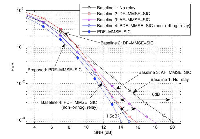
(a)

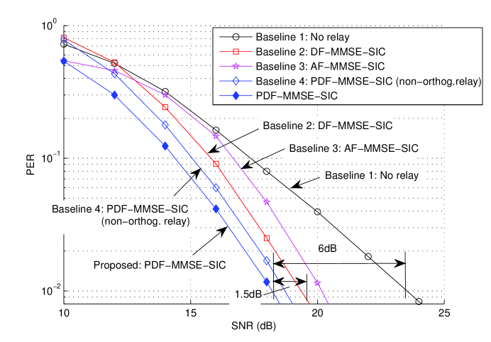
(b)

Figure 5: PER versus receive SNR comparison between the proposed PDF-MMSE-SIC scheme and baseline schemes. The source node is equipped with 4 antennas, whereas the relay and destination nodes are equipped with 2 antennas. We adopt the path loss models specified in Fig. 2: the source, relay and destination nodes are located according to the topology in Fig. 2 with $d_{SR}=400~{}\textrm{m}$, $d_{RD}=300~{}\textrm{m}$, and $d_{SD}=500~{}\textrm{m}$. (a) Performance with QPSK modulation. (b) Performance with 16-QAM modulation.

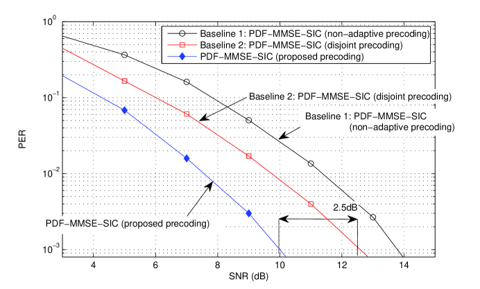
Figure 6: PER versus receive SNR comparison between the proposed precoding structure and baseline schemes. The source node is equipped with 4 antennas, whereas the relay and destination nodes are equipped with 2 antennas. The data streams are modulated using QPSK. We adopt the path loss models specified in Fig. 2: the source, relay and destination nodes are located according to the topology in Fig. 2 with $d_{SR}=400~{}\textrm{m}$, $d_{RD}=300~{}\textrm{m}$, and $d_{SD}=500~{}\textrm{m}$.

In this section, we provide numerical simulation results to assess the performance of the proposed PDF protocol (cf. Fig. 5) and MIMO precoder design (cf. Fig. 6).

For the purpose of illustration, we consider the following practical multi-antenna cooperative system with settings similar to those defined in the IEEE 802.16m standard [17]. We assume that uniform linear antenna arrays are used [27], where the source node has $n_{S}=4$ antennas, the relay node has $n_{R}=2$ antennas, and the destination node has $n_{D}=2$ antennas. At the source node, the data streams $\mathbf{s}^{(1)}$ and $\mathbf{s}^{(2)}$ are transmitted through $n_{S}^{(1)}=n_{S}^{(2)}=2$ diversity streams. We assume the source, the relay, and the destination nodes are located according to the topology in Fig. 2 with distances $d_{SR}=400~{}\textrm{m}$, $d_{RD}=300~{}\textrm{m}$, and $d_{SD}=500~{}\textrm{m}$. We evaluate performance using the end-to-end packet error rate (PER) versus SNR as metric. Specifically, we encode the data streams using the convolutional turbo code defined in the IEEE 802.16m standard [17, Section 16.3.11.1.5]: we assume each transmission phase lasts for $T=96$ symbol time slots, where each data stream contains $L=12$ information bytes coded at rate $1/2$ and modulated using QPSK or 16-QAM.

We show in Fig. 5 the performance of the proposed PDF protocol with non-adaptive precoding. We compare the proposed PDF-MMSE-SIC relay protocol against the following baselines.

• Baseline 1 (No relay): A relay node is not deployed and the destination node can only receive from the direct SD link, where the destination node uses MMSE-SIC receiver.

• Baseline 2 (DF MMSE-SIC): The relay node adopts the DF protocol (cf. (4b)), where the relay and destination nodes use MMSE-SIC receivers.

• Baseline 3 (AF MMSE-SIC): The relay node adopts the AF protocol (cf. (3)), where the relay and destination nodes use MMSE-SIC receivers.

• Baseline 4 (PDF MMSE-SIC with non-orthogonal relaying): The source node repeats transmission in both listening and cooperative phases [28], where the relay and destination nodes use MMSE-SIC receivers.

Let us focus on the performance with QPSK modulation (cf. Figure 5a). It can be seen that at PER of $10^{-3}$ the PDF-MMSE-SIC protocol has SNR gain in excess of 6 dB compared to when a relay node is not deployed, and has SNR gains of over 1.5 dB compared to conventional DF-MMSE-SIC and AF-MMSE-SIC schemes. The superior error performance by applying the PDF protocol is manifested from more effective mitigation of inter-stream interference at the destination node (compared to DF-MMSE-SIC and AF-MMSE-SIC) as well as enhanced probability that the relay node can assist with data transmission (compared to DF-MMSE-SIC). Note that it is inefficient to perform non-orthogonal relaying since transmission by the source node in the cooperative phase increases inter-stream interference in the decoding process at the destination node.

We demonstrate in Fig. 6 the effectiveness of the proposed precoding structure by comparing it with the following baselines:

• Baseline 1 (PDF-MMSE-SIC with non-adaptive precoding): The basic PDF protocol.

• Baseline 2 (PDF-MMSE-SIC with disjoint precoding): The source relay node precoders are determined in similar fashion as Theorem 1 and 2 but the total transmit power is evenly allocated between the source and relay nodes.

It can be seen that the proposed precoding structure yields better error performance than baselines 1 and 2 for all SNR regime. For instance, at PER of $10^{-3}$ the proposed precoder design has over 4 dB SNR gain over non-adaptive precoding (Baseline 1). Compared to disjoint precoding (Baseline 2), the proposed design achieves substantial advantage by adapting the power constraints of the source and relay nodes.

VI Conclusions

In this paper, we consider precoder design at the source and relay nodes for correlated multi-antenna cooperative systems that are matched to the PDF relay protocol and MMSE-SIC receivers. We derived the closed-form solution of the precoders at the source and relay nodes based on a primal decomposition approach. The performance of the proposed precoder designs is compared with several baselines and is shown to achieve significant performance gain compared to the baseline systems with MMSE-SIC receiver.

Appendix A: Proof of Lemma 1

We first show how to derive the mutual information for the SR link; in a similar fashion we can derive the mutual information for each PDF case. As per (1b), the source data streams $\textbf{s}^{(1)}$ and $\textbf{s}^{(2)}$ are respectively encoded into $\textbf{X}^{(1)}$ and $\textbf{X}^{(2)}$, and the received signals of the relay node are given by

$$\mathbf{Y}_{\!R,L}=\mathbf{H}_{SR}\,[\mathbf{P}_{\!S}]_{(:,1:n_{S}^{(1)})}\mathbf{X}^{(1)}+\mathbf{H}_{SR}\,[\mathbf{P}_{\!S}]_{(:,n_{S}^{(1)}+1:n_{\!S})}\mathbf{X}^{(2)}\!+\;\mathbf{Z}_{\!R,L}.$$ (25)

Suppose we decode $\textbf{s}^{(1)}$ first while treating $\textbf{s}^{(2)}$ as interference. Let $\lambda_{SR}^{(1)}=||\mathbf{H}_{SR}\,[\mathbf{P}_{\!S}]_{(:,1:n_{S}^{(1)})}||^{2}$ and $\lambda_{SR}^{(2)}=||\mathbf{H}_{SR}\,[\mathbf{P}_{\!S}]_{(:,n_{S}^{(1)}+1:n_{\!S})}||^{2}$. As shown in [29], after space-time processing the effective signal model for $\textbf{s}^{(1)}$ is $\textbf{y}_{\!R,L}^{(1)}=\lambda_{SR}^{(1)}\,\textbf{s}^{(1)}+\textbf{z}_{\!R,L}^{(1)}$, where $\textbf{z}_{\!R,L}^{(1)}$ denotes white Gaussian aggregate interference and noise terms with zero mean and variance$\lambda_{SR}^{(1)}\lambda_{SR}^{(2)}+\lambda_{SR}^{(1)}N_{0}$. Specifically, the noise variance is given by $||(\mathbf{H}_{SR}\,[\mathbf{P}_{\!S}]_{(:,1:n_{S}^{(1)})})^{{\dagger}}\;\mathbf{H}_{SR}\,[\mathbf{P}_{\!S}]_{(:,n_{S}^{(1)}+1:n_{\!S})}||^{2}+\lambda_{SR}^{(1)}N_{0}\leq\lambda_{SR}^{(1)}\lambda_{SR}^{(2)}+\lambda_{SR}^{(1)}N_{0}$. The SINR of $\textbf{s}^{(1)}$ is given by $\gamma_{\!R,L}^{(1)}=\frac{\lambda_{SR}^{(1)}}{\lambda_{SR}^{(2)}+N_{0}}$. Suppose $\textbf{s}^{(1)}$ is decoded as $\widehat{\textbf{s}}{\,}_{R}^{(1)}$ at SER $\epsilon_{R}$. We re-encode $\widehat{\textbf{s}}{\,}_{R}^{(1)}$ into $\widehat{\textbf{X}}^{(1)}$ and cancel it from the received signals $\mathbf{Y}_{\!R,L}$; the resultant signals are

$$\widetilde{\textbf{Y}}{}_{\!R,L}=\mathbf{H}_{SR}\,[\mathbf{P}_{\!S}]_{(:,n_{S}^{(1)}+1:n_{\!S})}\mathbf{X}^{(2)}+\mathbf{H}_{SR}\,[\mathbf{P}_{\!S}]_{(:,1:n_{S}^{(1)})}(\mathbf{X}^{(1)}-\widehat{\mathbf{X}}^{(1)})+\;\mathbf{Z}_{\!R,L}.$$ (26)

After space-time processing, we can express the effective signal model for data stream $\textbf{s}^{(2)}$ as $\textbf{y}_{\!R,L}^{(2)}=\lambda_{SR}^{(2)}\,\textbf{s}^{(2)}+\textbf{z}^{(2)}$, where $\textbf{z}^{(2)}$ denotes zero-mean white Gaussian aggregate residual interference and noise terms. The variance of $\textbf{z}^{(2)}$ depends on whether data stream $\textbf{s}^{(1)}$ is correctly decoded: if $\textbf{s}^{(1)}=\widehat{\textbf{s}}{\,}_{R}^{(1)}$, the variance of $\textbf{z}^{(2)}$ is given by $\lambda_{SR}^{(2)}N_{0}$; otherwise, the variance of $\textbf{z}^{(2)}$ is $4\epsilon_{R}\lambda_{SR}^{(2)}\lambda_{SR}^{(1)}+\lambda_{SR}^{(2)}N_{0}$. Specifically, the noise variance is given by

$||(\mathbf{H}_{SR}\,[\mathbf{P}_{\!S}]_{(:,n_{S}^{(1)}+1:n_{\!S})})^{{\dagger}}\;\mathbf{H}_{SR}\,[\mathbf{P}_{\!S}]_{(:,1:n_{S}^{(1)})}||^{2}\mathbb{E}(||\textbf{X}^{(1)}-\widehat{\textbf{X}}^{(1)}||^{2})+\lambda_{SR}^{(2)}N_{0}$.

If $\textbf{X}^{(1)}\!\neq\!\widehat{\textbf{X}}^{(1)}$, $\mathbb{E}(||\textbf{X}^{(1)}\!-\!\widehat{\textbf{X}}^{(1)}||^{2})\!\leq\!\mathbb{E}(||\textbf{X}^{(1)}||^{2})\!+\!\mathbb{E}(2\textrm{Re}(\textbf{X}^{(1)}(\widehat{\textbf{X}}^{(1)})^{{\dagger}}))\!+\!\mathbb{E}(||\widehat{\textbf{X}}^{(1)}||^{2})\!\leq\!4\mathbb{E}(||\textbf{X}^{(1)}||^{2})$. Hence, $\mathbb{E}(||\textbf{X}^{(1)}-\widehat{\textbf{X}}^{(1)}||^{2})\leq 4\epsilon_{R}$, and the noise variance can be expressed as $4\epsilon_{R}\lambda_{SR}^{(2)}\lambda_{SR}^{(1)}+\lambda_{SR}^{(2)}N_{0}$. Correspondingly, if $\textbf{s}^{(1)}=\widehat{\textbf{s}}{\,}_{R}^{(1)}$, the SINR of $\textbf{s}^{(2)}$ is given by $\gamma_{\!R,L}^{(2)}=\lambda_{SR}^{(2)}\,/\!N_{0}$; otherwise, the SINR of $\textbf{s}^{(2)}$ is given by $\gamma_{\!R,L}^{(2)}=\frac{\lambda_{SR}^{(2)}}{4\epsilon_{\!R}\lambda_{SR}^{(1)}+N_{0}}$. Therefore, the mutual information for $\textbf{s}^{(1)}$ is given by

$$\textstyle I(\mathbf{s}^{(1)};\mathbf{Y}_{\!R,L}\,|\,\mathbf{H}_{SR},\mathbf{P}_{\!S})=\log_{2}(1+\gamma_{\!R,L}^{(1)})=\log_{2}\!\bigg{(}\!1+\frac{\lambda_{SR}^{(1)}}{\lambda_{SR}^{(2)}+N_{0}}\bigg{)},$$ (27)

and the mutual information for $\textbf{s}^{(2)}$ is given by

$$I(\mathbf{s}^{(2)};\mathbf{Y}_{\!R,L}\,|\,\mathbf{H}_{SR},\mathbf{P}_{\!S},\widehat{\textbf{s}}{\,}_{R}^{(1)})=\log_{2}(1+\gamma_{\!R,L}^{(2)})= \;\;\;\;\;\log_{2}(1+\lambda_{SR}^{(2)}\,/\!N_{0}) \textbf{s}^{(1)}=\widehat{\textbf{s}}{\,}_{R}^{(1)}$$ ​​​​​​if , (28a)

$$I(\mathbf{s}^{(2)};\mathbf{Y}_{\!R,L}\,|\,\mathbf{H}_{SR},\mathbf{P}_{\!S},\widehat{\textbf{s}}{\,}_{R}^{(1)})=\log_{2}(1+\gamma_{\!R,L}^{(2)})= \textstyle\log_{2}\!\bigg{(}\!1+\frac{\lambda_{SR}^{(2)}}{4\epsilon_{\!R}\lambda_{SR}^{(1)}+N_{0}}\bigg{)}$$ ​​​​​​otherwise. (28b)

PDF Case 1: This case results when the relay node correctly decodes source data stream $\textbf{s}^{(1)}$. Let $D=2^{L/T}-1$. As per (27)-(28b) the probability of PDF Case 1 is given by

$$\textstyle\textrm{Pr}\,(\mathcal{A}_{1})=\textrm{Pr}\,\big{(}I(\mathbf{s}^{(1)};\mathbf{Y}_{\!R,L}\,|\,\mathbf{H}_{SR},\mathbf{P}_{\!S})\geq L/T\big{)}=\textrm{Pr}\bigg{(}\!\frac{\lambda_{SR}^{(1)}}{\lambda_{SR}^{(2)}+N_{0}}\geq D\bigg{)}.$$

Data stream $\textbf{s}^{(1)}$ is the cooperative stream and is forwarded by the relay node to the destination node. Combining the received signals in the listening and cooperative phases, it can be shown that the end-to-end mutual information for $\textbf{s}^{(1)}$ is ${I\!\;}_{\textrm{PDF}}^{(1)}(\mathcal{H},\mathbf{P}_{\!S},\mathbf{P}_{\!R})=\log_{2}\!\Bigg{(}\!1+\frac{\big{(}(\lambda_{SD}^{(1)})^{1\!/2}+(\lambda_{RD})^{1\!/2}\big{)}^{2}}{\lambda_{SD}^{(2)}+2N_{0}}\Bigg{)}$, where $\lambda_{SD}^{(1)}=||\mathbf{H}_{SD}\,[\mathbf{P}_{\!S}]_{(:,1:n_{S}^{(1)})}||^{2}$, $\lambda_{SD}^{(2)}=||\mathbf{H}_{SD}\,[\mathbf{P}_{\!S}]_{(:,n_{S}^{(1)}+1:n_{\!S})}||^{2}$, and $\lambda_{RD}=||\mathbf{H}_{RD}\,\mathbf{P}_{\!R}||^{2}$. Thus, the end-to-end outage probability of $\textbf{s}^{(1)}$ is $P_{\textrm{out}}^{(1)}(\mathbf{P}_{\!S},\mathbf{P}_{\!R}\,|\,\mathcal{A}_{1})=\textrm{Pr}\Bigg{(}\!\frac{\big{(}(\lambda_{SD}^{(1)})^{1\!/2}+(\lambda_{RD})^{1\!/2}\big{)}^{2}}{\lambda_{SD}^{(2)}+2N_{0}}<D\Bigg{)}$. On the other hand, data stream $\textbf{s}^{(2)}$ is the regular payload stream and is not forwarded by the relay node. Suppose the cooperative stream $\textbf{s}^{(1)}$ is decoded as $\widehat{\textbf{s}}{\,}_{D}^{(1)}$ at SER $\epsilon_{\mathcal{A}_{1}}\!$ and we cancel its interference from the SD link received signals. If $\textbf{s}^{(1)}=\widehat{\textbf{s}}{\,}_{D}^{(1)}$, then the end-to-end mutual information for $\textbf{s}^{(2)}$ is ${I\!\;}_{\textrm{PDF}}^{(2)}(\mathcal{H},\mathbf{P}_{\!S},\mathbf{P}_{\!R})=\log_{2}(1+\lambda_{SD}^{(2)}\,/\!N_{0})$; otherwise, the end-to-end mutual information for $\textbf{s}^{(2)}$ is ${I\!\;}_{\textrm{PDF}}^{(2)}(\mathcal{H},\mathbf{P}_{\!S},\mathbf{P}_{\!R})=\log_{2}\!\bigg{(}\!1+\frac{\lambda_{SD}^{(2)}}{4\,\epsilon_{\!\mathcal{A}_{1}}\!\lambda_{SD}^{(1)}+N_{0}}\bigg{)}$. Therefore, the end-to-end outage probability of $\textbf{s}^{(2)}$ is

$P_{\textrm{out}}^{(2)}(\mathbf{P}_{\!S},\mathbf{P}_{\!R}|\,\mathcal{A}_{1})\!=\!(1\!-\!P_{\textrm{out}}^{(1)}(\mathbf{P}_{\!S},\mathbf{P}_{\!R}|\,\mathcal{A}_{1}))\,\textrm{Pr}\,(\lambda_{SD}^{(2)}\!<\!D)\!+\!P_{\textrm{out}}^{(1)}(\mathbf{P}_{\!S},\mathbf{P}_{\!R}|\,\mathcal{A}_{1})\,\textrm{Pr}\bigg{(}\!\frac{\lambda_{SD}^{(2)}}{4\,\epsilon_{\!\mathcal{A}_{1}}\!\lambda_{SD}^{(1)}+N_{0}}\!<\!D\bigg{)}$.

PDF Case 2: This case results when the relay node incorrectly decodes source data stream $\mathbf{s}^{(1)}$ but correctly decodes data stream $\mathbf{s}^{(2)}$. As per (27)-(28b), the probability of PDF Case 2 is

$$\textstyle\textrm{Pr}\,(\mathcal{A}_{2})\; \textstyle=\textrm{Pr}\,\big{(}I(\mathbf{s}^{(1)};\mathbf{Y}_{\!R,L}\,|\,\mathbf{H}_{SR},\mathbf{P}_{\!S})<L/T\big{)}\,\textrm{Pr}\,\big{(}I(\mathbf{s}^{(2)};\mathbf{Y}_{\!R,L}\,|\,\mathbf{H}_{SR},\mathbf{P}_{\!S},\textbf{s}^{(1)}\neq\widehat{\textbf{s}}{\,}_{R}^{(1)})\geq L/T\big{)}$$

$$\textstyle=\textrm{Pr}\bigg{(}\!\frac{\lambda_{SR}^{(1)}}{\lambda_{SR}^{(2)}+N_{0}}<D\bigg{)}\,\textrm{Pr}\bigg{(}\!\frac{\lambda_{SR}^{(2)}}{4\epsilon_{\!R}\lambda_{SR}^{(1)}+N_{0}}\geq D\bigg{)}.$$

We can derive the outage probabilities of $\textbf{s}^{(1)}$ and $\textbf{s}^{(2)}$ analogous to PDF Case 1, but instead we treat $\textbf{s}^{(1)}$ as the regular payload stream and $\textbf{s}^{(2)}$ as the cooperative stream.

PDF Case 3: This case results when the relay node incorrectly decodes both source data streams $\mathbf{s}^{(1)}$ and $\mathbf{s}^{(2)}$. As per (27)-(28b), the probability of PDF Case 3 is given by

$$\textstyle\textrm{Pr}\,(\mathcal{A}_{3})\; \textstyle=\textrm{Pr}\,\big{(}I(\mathbf{s}^{(1)};\mathbf{Y}_{\!R,L}\,|\,\mathbf{H}_{SR},\mathbf{P}_{\!S})<L/T\big{)}\,\textrm{Pr}\,\big{(}I(\mathbf{s}^{(2)};\mathbf{Y}_{\!R,L}\,|\,\mathbf{H}_{SR},\mathbf{P}_{\!S},\textbf{s}^{(1)}\neq\widehat{\textbf{s}}{\,}_{R}^{(1)})<L/T\big{)}$$

$$\textstyle=\textrm{Pr}\bigg{(}\!\frac{\lambda_{SR}^{(1)}}{\lambda_{SR}^{(2)}+N_{0}}<D\bigg{)}\,\textrm{Pr}\bigg{(}\!\frac{\lambda_{SR}^{(2)}}{4\epsilon_{\!R}\lambda_{SR}^{(1)}+N_{0}}<D\bigg{)}.$$

Since neither $\mathbf{s}^{(1)}$ nor $\mathbf{s}^{(2)}$ is forwarded by the relay node, at the destination node we decode the data streams only from the SD link received signals. The mutual information for each data stream can be determined similar to the derivation of (27)-(28b) focusing instead on the SD link.

Appendix B: Proof of Theorem 1

For analytical tractability, we assume that under PDF Case 1 and 2 the SER of the cooperative stream is reasonably low (e.g. $\epsilon_{\mathcal{A}_{1}},\epsilon_{\mathcal{A}_{2}}\ll 1$), and the outage probabilities of the regular payload stream under PDF Case 1 and 2 can be approximated as:

$$P_{\textrm{out}}^{(2)}(\mathbf{P}_{\!S},\mathbf{P}_{\!R}\,|\,\mathcal{A}_{1})\!\approx\textrm{Pr}\,(\lambda_{SD}^{(2)}\,/\!N_{0}\!<D)\;\;\textrm{and}\;\;P_{\textrm{out}}^{(1)}(\mathbf{P}_{\!S},\mathbf{P}_{\!R}\,|\,\mathcal{A}_{2})\!\approx\textrm{Pr}\,(\lambda_{SD}^{(1)}\,/\!N_{0}\!<D).\;\;\;\;\;\;$$ (29)

Thus, the average end-to-end per-stream outage probability $P_{\textrm{out}}(\mathbf{P}_{\!S},\mathbf{P}_{\!R})$ is related to the relay node precoder $\mathbf{P}_{\!R}$ only w.r.t. the probabilities $P_{\textrm{out}}^{(1)}(\mathbf{P}_{\!S},\mathbf{P}_{\!R}\,|\,\mathcal{A}_{1})\!\!<\textrm{Pr}\Big{(}\!\lambda_{RD}\!<\!(\lambda_{SD}^{(2)}\!+\!2N_{0})D\!-\!\lambda_{SD}^{(1)}\Big{)}$ and $P_{\textrm{out}}^{(2)}(\mathbf{P}_{\!S},\mathbf{P}_{\!R}\,|\,\mathcal{A}_{2})\!\!<\textrm{Pr}\Big{(}\!\lambda_{RD}\!<\!(\lambda_{SD}^{(1)}\!+\!2N_{0})D\!-\!\lambda_{SD}^{(2)}\Big{)}$. To minimize $P_{\textrm{out}}^{(1)}(\mathbf{P}_{\!S},\mathbf{P}_{\!R}\,|\,\mathcal{A}_{1})$ and $P_{\textrm{out}}^{(2)}(\mathbf{P}_{\!S},\mathbf{P}_{\!R}\,|\,\mathcal{A}_{2})$, we design $\mathbf{P}_{\!R}$ to minimize the probability density function (p.d.f.) of $\lambda_{RD}$.

The p.d.f. of $\lambda_{RD}$ is given as follows. By definition, $\lambda_{RD}=||\mathbf{H}_{RD}\,\mathbf{P}_{\!R}||^{2}=(\mathbf{g}_{RD})^{\!{\dagger}}\mathbf{g}_{RD}$, where $\mathbf{g}_{RD}=\textrm{vec}(\mathbf{H}_{RD}\,\mathbf{P}_{\!R})\stackrel{{\scriptstyle(a)}}{{=}}((\mathbf{P}_{\!R})^{T}(\mathbf{\Lambda}_{RD,t})^{\!1\!\!\>/\!\>2}\otimes(\mathbf{\Lambda}_{RD,r})^{\!1\!\!\>/\!\>2})\,\textrm{vec}(\mathbf{G}_{\!RD})$ and (a) follows from (5). Since the entries of $\mathbf{G}_{\!RD}$ are i.i.d. complex Gaussian with zero mean and unit variance, $\mathbf{g}_{RD}$ is multivariate Gaussian distributed whose p.d.f. is given by $p(\mathbf{g}_{RD})=\frac{\exp(-(\mathbf{g}_{RD})^{{\dagger}}\mathbf{\Omega}^{-1}\mathbf{g}_{RD})}{(2\pi)^{V}\det(\mathbf{\Omega})}$, where $V=n_{\!D}n_{\!R}$, $\mathbf{\Omega}=(\mathbf{P}_{\!R})^{T}\mathbf{\Xi}_{RD,t}(\mathbf{P}_{\!R})^{\ast}\otimes\mathbf{\Xi}_{RD,r}$, $\mathbf{\Xi}_{RD,t}=(\mathbf{\Lambda}_{RD,t})^{\!1\!\!\>/\!\>2}((\mathbf{\Lambda}_{RD,t})^{\!1\!\!\>/\!\>2})^{{\dagger}}$, and $\mathbf{\Xi}_{RD,r}=(\mathbf{\Lambda}_{RD,r})^{\!1\!\!\>/\!\>2}((\mathbf{\Lambda}_{RD,r})^{\!1\!\!\>/\!\>2})^{{\dagger}}$. Let $\mathbf{\Omega}^{-1}=\textbf{U}_{\mathbf{\Omega}}(\mathbf{\Sigma}_{\mathbf{\Omega}})^{-1}(\textbf{U}_{\mathbf{\Omega}})^{{\dagger}}$ denote the eigendecomposition of $\mathbf{\Omega}^{-1}$, where $\mathbf{\Sigma}_{\mathbf{\Omega}}=\textrm{diag}(\delta_{\max},\ldots,\delta_{\min})$ with $\delta_{\max}$ and $\delta_{\min}$ denote the maximum and minimum eigenvalues of $\mathbf{\Omega}$. Hence, $(\mathbf{g}_{RD})^{{\dagger}}\mathbf{\Omega}^{-1}\mathbf{g}_{RD}\geq(\mathbf{g}_{RD})^{{\dagger}}\textbf{U}_{\mathbf{\Omega}}\big{(}\frac{1}{\delta_{\max}}\textbf{I}_{V}\big{)}(\textbf{U}_{\mathbf{\Omega}})^{{\dagger}}\mathbf{g}_{RD}=\frac{1}{\delta_{\max}}(\mathbf{g}_{RD})^{{\dagger}}\mathbf{g}_{RD}$ and the p.d.f. of $\lambda_{RD}$ is upper bounded by $p(\lambda_{RD})\leq\frac{\exp(-\lambda_{RD}/\delta_{\max})}{(2\pi)^{V}(\delta_{\min})^{V}}$.

To minimize the p.d.f. of $\lambda_{RD}$ (and thereby minimize $P_{\textrm{out}}(\mathbf{P}_{\!S},\mathbf{P}_{\!R})$), we seek to minimize $\delta_{\max}$ and maximize $\delta_{\min}$; this implies minimizing the condition number of $\mathbf{\Omega}$, $\chi(\mathbf{\Omega})=\frac{\delta_{\max}}{\delta_{\min}}$. It can be shown that $\chi(\mathbf{\Omega})=\chi((\mathbf{P}_{\!R})^{T}\mathbf{\Xi}_{RD,t}(\mathbf{P}_{\!R})^{\ast}\otimes\mathbf{\Xi}_{RD,r})=\chi((\mathbf{P}_{\!R})^{T}\mathbf{\Xi}_{RD,t}(\mathbf{P}_{\!R})^{\ast})\chi(\mathbf{\Xi}_{RD,r})$. Therefore, we recast subproblem (18) as

$$\min_{\mathbf{P}_{\!R}}\chi((\mathbf{P}_{\!R})^{T}\mathbf{\Xi}_{RD,t}(\mathbf{P}_{\!R})^{\ast}),\;\;\textrm{s.t.}\;\;||\mathbf{P}_{\!R}||^{2}\leq\alpha_{R}.$$ (30)

Let $\mathbf{\Xi}_{RD,t}=\mathbf{U}_{\!RD,t}\mathbf{\Sigma}_{\!RD,t}(\mathbf{U}_{\!RD,t})^{{\dagger}}$ denote the eigendecomposition of $\mathbf{\Xi}_{RD,t}$, and the solution to (30) is given by $\mathbf{P}_{\!R}^{\star}=\sqrt{\frac{\alpha_{R}}{\textrm{Tr}\,((\mathbf{\Sigma}_{\!RD,t})^{-1})}}\,(\mathbf{U}_{\!RD,t})^{\ast}\,(\mathbf{\Sigma}_{\!RD,t})^{-1/2}$. The physical meaning of this precoder design is to equalize the RD link transmit-side correlation matrix.

Appendix C: Proof of Theorem 2

The probability of PDF Case 3 can be upper bounded as

$$\textrm{Pr}\,(\mathcal{A}_{3})\; \textstyle=\textrm{Pr}\bigg{(}\!\frac{\lambda_{SR}^{(1)}}{\lambda_{SR}^{(2)}+N_{0}}<2^{L/T}-1\bigg{)}\,\textrm{Pr}\bigg{(}\!\frac{\lambda_{SR}^{(2)}}{4\epsilon_{\!R}\lambda_{SR}^{(1)}+N_{0}}<2^{L/T}-1\bigg{)}$$

$$\textstyle<C(\epsilon_{R},D)\textrm{Pr}\Big{(}\!\frac{\lambda_{SR}^{(2)}}{4\epsilon_{\!R}D}-\frac{N_{0}}{4\epsilon_{\!R}}<\lambda_{SR}^{(1)}<\lambda_{SR}^{(2)}D+D\Big{)}$$

$$\textstyle=C(\epsilon_{R},D)\int_{k=0}^{\infty}\textrm{Pr}\Big{(}\!\frac{k}{4\epsilon_{\!R}D}-\frac{N_{0}}{4\epsilon_{\!R}}<\lambda_{SR}^{(1)}<kD+D\Big{)}\textrm{Pr}(\lambda_{SR}^{(2)}=k)dk,$$

where $D=2^{L/T}-1$ is the data rate, and $C(\epsilon_{R},D)$ is a constant that is a function of the SER $\epsilon_{R}$ and $D$. To minimize (Appendix C: Proof of Theorem 2), we seek to design the source precoder $\mathbf{P}_{\!S}$ to minimize the inner probability expression for given $k$:

$$\min_{\mathbf{P}_{\!S}}\textstyle\textrm{Pr}\Big{(}\!\frac{k}{4\epsilon_{\!R}D}-\frac{N_{0}}{4\epsilon_{\!R}}<\lambda_{SR}^{(1)}<kD+D\Big{)}\textrm{Pr}(\lambda_{SR}^{(2)}=k),\;\;\textrm{s.t.}\;\;||\mathbf{P}_{\!S}||^{2}\leq\alpha_{S}.$$ (33)

We solve (33) by first deriving the precoder structure that minimizes the joint p.d.f. of $\lambda_{SR}^{(1)}$ and $\lambda_{SR}^{(2)}$, and the p.d.f. is given as follows. By definition, $\lambda_{SR}^{(1)}=||\mathbf{H}_{SR}\,[\mathbf{P}_{\!S}]_{(:,1:n_{S}^{(1)})}||^{2}$ and $\lambda_{SR}^{(2)}=||\mathbf{H}_{SR}\,[\mathbf{P}_{\!S}]_{(:,n_{S}^{(1)}+1:n_{\!S})}||^{2}$; let $\lambda_{SR}=\lambda_{SR}^{(1)}+\lambda_{SR}^{(2)}=||\mathbf{H}_{SR}\,\mathbf{P}_{\!S}||^{2}=(\mathbf{g}_{SR})^{\!{\dagger}}\mathbf{g}_{SR}$, where $\mathbf{g}_{RD}=\textrm{vec}(\mathbf{H}_{RD}\,\mathbf{P}_{\!R})$. It can be shown, in analogy to the proof of Theorem 1, that the p.d.f. of $\mathbf{g}_{SR}$ is $p(\mathbf{g}_{SR})=\frac{\exp(-(\mathbf{g}_{SR})^{{\dagger}}\mathbf{\Phi}^{-1}\mathbf{g}_{SR})}{(2\pi)^{W}\det(\mathbf{\Phi})}$, where $W=n_{\!R}n_{\!S}$, $\mathbf{\Phi}=(\mathbf{P}_{\!S})^{T}\mathbf{\Xi}_{SR,t}(\mathbf{P}_{\!S})^{\ast}\otimes\mathbf{\Xi}_{SR,r}$, $\mathbf{\Xi}_{SR,t}=(\mathbf{\Lambda}_{SR,t})^{\!1\!\!\>/\!\>2}((\mathbf{\Lambda}_{SR,t})^{\!1\!\!\>/\!\>2})^{{\dagger}}$, and $\mathbf{\Xi}_{SR,r}=(\mathbf{\Lambda}_{SR,r})^{\!1\!\!\>/\!\>2}((\mathbf{\Lambda}_{SR,r})^{\!1\!\!\>/\!\>2})^{{\dagger}}$. Let $\mathbf{\Xi}_{SR,t}=\mathbf{U}_{\!SR,t}\mathbf{\Sigma}_{\!SR,t}(\mathbf{U}_{\!SR,t})^{{\dagger}}$ denote the eigendecomposition of $\mathbf{\Xi}_{SR,t}$. Without loss of generality, let the source node precoder be given by

$$\mathbf{P}_{\!S}=\sqrt{\alpha_{S}}\,(\mathbf{U}_{\!SR,t})^{\ast}\,\mathbf{\Sigma}_{S},$$ (34)

where $\mathbf{\Sigma}_{S}$ is a diagonal matrix. Thus, $\mathbf{\Phi}=\alpha_{S}\mathbf{\Sigma}_{S}\mathbf{\Sigma}_{\!SR,t}\mathbf{\Sigma}_{S}\otimes\mathbf{\Xi}_{SR,r}=\Bigg{[}\!\!\begin{array}[]{cc}\mathbf{\Phi}^{(1)}\!\!\!\!&\textbf{0}\\ \textbf{0}\!\!\!\!&\mathbf{\Phi}^{(2)}\end{array}\!\!\Bigg{]}$ with $\mathbf{\Phi}^{(1)}=\alpha_{S}[\mathbf{\Sigma}_{S}\mathbf{\Sigma}_{\!SR,t}\mathbf{\Sigma}_{S}]_{(1:n_{S}^{(1)},1:n_{S}^{(1)})}\otimes\mathbf{\Xi}_{SR,r}$ and $\mathbf{\Phi}^{(2)}=\alpha_{S}[\mathbf{\Sigma}_{S}\mathbf{\Sigma}_{\!SR,t}\mathbf{\Sigma}_{S}]_{(n_{S}^{(1)}+1:n_{\!S},n_{S}^{(1)}+1:n_{\!S})}\otimes\mathbf{\Xi}_{SR,r}$, and the p.d.f. of $\mathbf{g}_{SR}$ can be expressed as

$$\textstyle p(\mathbf{g}_{SR})=\frac{\exp(-([\mathbf{g}_{SR}]_{(1:W^{(1)})})^{{\dagger}}(\mathbf{\Phi}^{(1)})^{-1}[\mathbf{g}_{SR}]_{(1:W^{(1)})})}{(2\pi)^{W^{(1)}}\det(\mathbf{\Phi}^{(1)})}\frac{\exp(-([\mathbf{g}_{SR}]_{(W^{(1)}+1:W)})^{{\dagger}}(\mathbf{\Phi}^{(2)})^{-1}[\mathbf{g}_{SR}]_{(W^{(1)}+1:W)})}{(2\pi)^{W^{(2)}}\det(\mathbf{\Phi}^{(2)})}$$

for $W^{(1)}=n_{\!R}n_{\!S}^{(1)}$ and $W^{(2)}=n_{\!R}n_{\!S}^{(2)}$. Let $(\mathbf{\Phi}^{(i)})^{-1}=\textbf{U}_{\mathbf{\Phi}^{(1)}}(\mathbf{\Sigma}_{\mathbf{\Phi}^{(i)}})^{-1}(\textbf{U}_{\mathbf{\Phi}^{(i)}})^{{\dagger}}$ denote the eigendecomposition of $(\mathbf{\Phi}^{(i)})^{-1}$, where $\mathbf{\Sigma}_{\mathbf{\Phi}^{(i)}}=\textrm{diag}(\delta_{\max}^{(i)},\ldots,\delta_{\min}^{(i)})$ with $\delta_{\max}^{(i)}$ and $\delta_{\min}^{(i)}$ denote, respectively, the the maximum and minimum eigenvalues of $\mathbf{\Phi}^{(i)}$. Therefore, the joint p.d.f. of $\lambda_{SR}^{(1)}$ and $\lambda_{SR}^{(2)}$ is upper bounded by $p(\lambda_{SR}^{(1)},\lambda_{SR}^{(2)})=p(\lambda_{SR}^{(1)})p(\lambda_{SR}^{(2)})$, where $p(\lambda_{SR}^{(1)})\leq\frac{\exp(-\lambda_{SR}^{(1)}/\delta_{\max}^{(1)})}{(2\pi)^{W^{(1)}}(\delta_{\min}^{(1)})^{W^{(1)}}}$ and $p(\lambda_{SR}^{(2)})\leq\frac{\exp(-\lambda_{SR}^{(2)}/\delta_{\max}^{(2)})}{(2\pi)^{W^{(2)}}(\delta_{\min}^{(2)})^{W^{(2)}}}$.

Since the joint p.d.f. of $\lambda_{SR}^{(1)}$ and $\lambda_{SR}^{(2)}$ is separable, we decompose and the precoder design problem (33) as follows. Let $\rho_{S}^{(1)},\rho_{S}^{(2)}\geq 0$, $\rho_{S}^{(1)}+\rho_{S}^{(2)}=1$, be power allocation variables (which we address subsequently), and we can recast (33) as

$$\min_{\mathbf{P}_{\!S}}\textstyle\textrm{Pr}\Big{(}\!\frac{k}{4\epsilon_{\!R}D}-\frac{N_{0}}{4\epsilon_{\!R}}<\lambda_{SR}^{(1)}<kD+D\Big{)},\;\;\textrm{s.t.}\;\;||[\mathbf{P}_{\!S}]_{(:,1:n_{S}^{(1)})}||^{2}\leq\rho_{S}^{(1)}\alpha_{S},$$

$$\min_{\mathbf{P}_{\!S}}\textstyle\textrm{Pr}(\lambda_{SR}^{(2)}=k),\;\;\textrm{s.t.}\;\;||[\mathbf{P}_{\!S}]_{(:,n_{S}^{(1)}+1:n_{\!S})}||^{2}\leq\rho_{S}^{(2)}\alpha_{S},$$

To solve (Appendix C: Proof of Theorem 2) we seek to minimize the condition number of $\mathbf{\Phi}^{(1)}$, and similarly to solve (Appendix C: Proof of Theorem 2) we seek to minimize the condition number of $\mathbf{\Phi}^{(2)}$. As per (34), the solution to (Appendix C: Proof of Theorem 2) is given by

$$\mathbf{P}_{\!S}^{\star}=\sqrt{\alpha_{S}}\,(\mathbf{U}_{\!SR,t})^{\ast}\!\left[\!\!\begin{array}[]{cc}\sqrt{\frac{\rho_{S}^{(1)}}{\textrm{Tr}\,((\mathbf{\Sigma}_{\!SR,t}^{(1)})^{-1})}}(\mathbf{\Sigma}_{\!SR,t}^{(1)})^{-1/2}\!\!\!\!\!\!&\textbf{0}\\ \textbf{0}\!\!\!\!\!\!&\sqrt{\frac{\rho_{S}^{(2)}}{\textrm{Tr}\,((\mathbf{\Sigma}_{\!SR,t}^{(2)})^{-1})}}(\mathbf{\Sigma}_{\!SR,t}^{(2)})^{-1/2}\end{array}\!\!\right],$$

where $\mathbf{\Sigma}_{\!SR,t}^{(1)}$ = $[\mathbf{\Sigma}_{\!SR,t}]_{(1:n_{S}^{(1)},1:n_{S}^{(1)})}$ and $\mathbf{\Sigma}_{\!SR,t}^{(2)}$ = $[\mathbf{\Sigma}_{\!SR,t}]_{(n_{S}^{(1)}+1:n_{\!S},n_{S}^{(1)}+1:n_{\!S})}$.

Given the precoder structure in (Appendix C: Proof of Theorem 2), we recast (33) to solve for the power allocation variables $\rho_{S}^{(1)}$ and $\rho_{S}^{(2)}$. The probabilities in (Appendix C: Proof of Theorem 2) are given by

$$\textstyle\textrm{Pr}\Big{(}\!\frac{k}{4\epsilon_{\!R}D}\!-\!\frac{N_{0}}{4\epsilon_{\!R}}\!<\!\lambda_{SR}^{(1)}\!<\!kD\!+\!D\Big{)}\leq\frac{\delta_{\max}^{(1)}}{(2\pi)^{W^{(1)}}(\delta_{\min}^{(1)})^{W^{(1)}}}\left(\!\exp\!\left(\!-\frac{\frac{k}{4\epsilon_{\!R}D}-\frac{N_{0}}{4\epsilon_{\!R}}}{\delta_{\max}^{(1)}}\right)-\exp\!\left(\!-\frac{kD+D}{\delta_{\max}^{(1)}}\right)\!\right),\;\;\;\;\;\;$$

$$\textstyle\textrm{Pr}(\lambda_{SR}^{(2)}=k)\leq\frac{\exp(-k/\delta_{\max}^{(2)})}{(2\pi)^{W^{(2)}}(\delta_{\min}^{(2)})^{W^{(2)}}},$$

where $\delta_{\max}^{(1)}=\frac{\rho_{S}^{(1)}\alpha_{S}\sigma_{\max}(\mathbf{\Xi}_{SR,r})}{\textrm{Tr}\,((\mathbf{\Sigma}_{\!SR,t}^{(1)})^{-1})}$, $\delta_{\min}^{(1)}=\frac{\rho_{S}^{(1)}\alpha_{S}\sigma_{\min}(\mathbf{\Xi}_{SR,r})}{\textrm{Tr}\,((\mathbf{\Sigma}_{\!SR,t}^{(1)})^{-1})}$, $\delta_{\max}^{(2)}=\frac{\rho_{S}^{(2)}\alpha_{S}\sigma_{\max}(\mathbf{\Xi}_{SR,r})}{\textrm{Tr}\,((\mathbf{\Sigma}_{\!SR,t}^{(2)})^{-1})}$, and $\delta_{\min}^{(2)}=\frac{\rho_{S}^{(2)}\alpha_{S}\sigma_{\min}(\mathbf{\Xi}_{SR,r})}{\textrm{Tr}\,((\mathbf{\Sigma}_{\!SR,t}^{(2)})^{-1})}$. Substituting (Appendix C: Proof of Theorem 2) into (33), and let $\widetilde{\delta}^{(1)}=\frac{\delta_{\max}^{(1)}}{\rho_{S}^{(1)}}$ and $\widetilde{\delta}^{(2)}=\frac{\delta_{\max}^{(2)}}{\rho_{S}^{(2)}}$, we have

$$\min_{\rho_{S}^{(1)},\rho_{S}^{(2)}\geq 0}\textstyle\frac{\exp\left(-\frac{k}{\rho_{S}^{(2)}\widetilde{\delta}^{(2)}}\right)}{(\rho_{S}^{(2)})^{W^{(2)}}(\rho_{S}^{(2)})^{W^{(1)}-1}}\left(\!\exp\!\left(\!-\frac{\frac{k}{4\epsilon_{\!R}D}-\frac{N_{0}}{4\epsilon_{\!R}}}{\rho_{S}^{(1)}\widetilde{\delta}^{(1)}}\right)-\exp\!\left(\!-\frac{kD+D}{\rho_{S}^{(1)}\widetilde{\delta}^{(1)}}\right)\!\right)$$

$$\;\;\;\;\textrm{s.t.}\;\;\;\;\;\rho_{S}^{(1)}\!+\!\rho_{S}^{(2)}\!\leq\!1.\;\;$$

Finally, we can determine $\rho_{S}^{(1)}$ and $\rho_{S}^{(2)}$ as follows. Substitute $\rho_{S}^{(2)}=1-\rho_{S}^{(1)}$ into (Appendix C: Proof of Theorem 2) and take the first order derivative w.r.t. $\rho_{S}^{(1)}$ whose roots give the optimal value of $\rho_{S}^{(1)}$ and they can be found using, for example, bisection search or Newton’s algorithm [26]. After that, it is straightforward to determine $\rho_{S}^{(2)}$.

References

• [1] J. N. Laneman, D. N. C. Tse, and G. W. Wornell, “Cooperative diversity in wireless networks: Efficient protocols and outage behavior,” IEEE Trans. Inf. Theory, vol. 50, pp. 3062–3080, Dec. 2004.
• [2] A. S. Avestimehr and D. N. C. Tse, “Outage capacity of the fading relay channel in the low SNR regime,” IEEE Trans. Inf. Theory, vol. 53, pp. 1401–1415, Apr. 2007.
• [3] K. Azarian, H. E. Gamal, and P. Schniter, “On the achievable diversity multiplexing tradeoff in half-duplex cooperative channels,” IEEE Trans. Inf. Theory, vol. 51, pp. 4152–4172, Dec. 2005.
• [4] M. Yuksel and E. Erkip, “Broadcast strategies for the fading relay channel,” in Proc. IEEE MILCOM’04, 2004.
• [5] Y. Ding, J.-K. Zhang, and K. Wong, “Optimal precoder for amplify-and-forward half-duplex relay system,” IEEE Trans. Wireless Commun., vol. 7, pp. 2890–2895, Aug. 2008.
• [6] X. Tang and Y. Hua, “Optimal design of non-regenerative MIMO wireless relays,” IEEE Trans. Wireless Commun., vol. 6, pp. 1398–1407, Apr. 2007.
• [7] O. Munoz, J. Vidal, and A. Agustin, “Non-regenerative MIMO relaying with channel state information,” in Proc. IEEE ICASSP’05, Mar. 2005.
• [8] C. Xing, S. Ma, and Y.-C. Wu, “Robust joint design of linear relay precoder and destination equalizer for dual-hop amplify-and-forward MIMO relay systems,” IEEE Trans. Signal Process., vol. 58, pp. 2273–2283, Apr. 2010.
• [9] B. Khoshnevis, W. Yu, and R. Adve, “Grassmannian beamforming for MIMO amplify-and-forward relaying,” IEEE J. Sel. Areas Commun., vol. 26, pp. 1397–1407, Oct. 2008.
• [10] S. S. Lokesh, A. Kumar, and M. Agrawal, “Structure of an optimum linear precoder and its application to ML equalizer,” IEEE Trans. Signal Process., vol. 56, pp. 3690–3701, Aug. 2008.
• [11] A. Sezgin, A. Paulraj, and M. Vu, “Impact of correlation on linear precoding in QSTBC coded systems with linear MSE detection,” in Proc. IEEE GLOBECOM’07, Nov. 2007.
• [12] C. Meng and J. Tuqan, “Precoded STBC-VBLAST for MIMO wireless communication systems,” in Proc. IEEE ICASSP’07, 2007.
• [13] S. Alamouti, “A simple transmit diversity technique for wireless communications,” IEEE J. Sel. Areas Commun., vol. 16, pp. 1451–1458, Oct. 1998.
• [14] V. Tarokh, H. Jafarkhani, and A. R. Calderbank, “Space-time block codes from orthogonal designs,” IEEE Trans. Inf. Theory, vol. 45, pp. 744–765, Jul. 1999.
• [15] H. Jafarkhani, “A quasi orthogonal space-time block code,” IEEE Trans. Commun., vol. 49, pp. 1–4, Jan. 2001.
• [16] A. Pascual-Iserte, D. P. Palomar, A. I. Prez-Neira, and M. A. Lagunas, “A robust maximin approach for MIMO communications with partial channel state information based on convex optimization,” IEEE Trans. Signal Process., vol. 54, pp. 346–360, Jan. 2006.
• [17] Draft Amendment to IEEE Standard for Local and Metropolitan Area Networks, Part 16: Air Interface for Fixed and Mobile Broadband Wireless Access Systems, IEEE Std. P802.16m/D10, 2010.
• [18] W. Weichselberger, M. Herlin, H. Ozcelik, and E. Bonek, “A stochastic MIMO channel model with joint correlation of both link ends,” IEEE Trans. Wireless Commun., vol. 5, pp. 90–100, Jan. 2006.
• [19] G. J. Foschini, G. D. Golden, R. A. Valenzuela, and P. W. Wolniansky, “Simplified processing for high spectral efficiency wireless communication employing multi-element arrays,” IEEE Trans. Commun., vol. 17, pp. 1841–1852, Nov. 1999.
• [20] S. Senthuran, A. Anpalagan, and O. Das, “Cooperative subcarrier and power allocation for a two-hop decode-and-forward OFCDM based relay network,” IEEE Trans. Wireless Commun., vol. 8, pp. 4797–4805, Sep. 2009.
• [21] M. Chen, S. Serbetli, and A. Yener, “Distributed power allocation strategies for parallel relay networks,” IEEE Trans. Wireless Commun., vol. 7, pp. 552–561, Feb. 2008.
• [22] N. Zhou, X. Zhu, Y. Huang, and H. Lin, “Adaptive resource allocation for multi-destination relay systems based on OFDM modulation,” in Proc. IEEE ICC’09, Jun. 2009.
• [23] D. P. Palomar, J. M. Cioffi, and M. A. Lagunas, “Joint Tx-Rx beamforming design for multicarrier MIMO channels: A unified framework for convex optimization,” IEEE Trans. Signal Process., vol. 51, pp. 2381–2401, Sep. 2003.
• [24] H. Sampath and A. Paulraj, “Linear precoding for space-time coded systems with known fading correlations,” IEEE Commun. Lett., vol. 6, pp. 239–241, Jun. 2002.
• [25] H. R. Bahrami and T. Le-Ngoc, “Precoder design based on correlation matrices for mimo systems,” IEEE Trans. Wireless Commun., vol. 5, pp. 3579–3587, Dec. 2006.
• [26] S. Boyd and L. Vandenberghe, Convex Optimization.   Cambridge University Press, 2003.
• [27] IEEE 802.16m evaluation methodology document. IEEE 802.16m-08/004r4.
• [28] R. U. Nabar, H. B$\ddot{\textrm{o}}$lcskei, and F. W. Kneub$\ddot{\textrm{u}}$hler, “Fading relay channels: Performance limits and space-time signal design,” IEEE J. Sel. Areas Commun., vol. 22, pp. 1099–1109, Aug. 2004.
• [29] G. Ganesan and P. Stoica, “Space-time block codes: A maximum SNR approach,” IEEE Trans. Inf. Theory, vol. 47, pp. 1650–1656, May 2001.
Refer to caption