Non-local correlations in the Haldane phase for an XXZ spin-1 chain: A perspective from infinite matrix product state representation

Abstract

String correlations are investigated in an infinite-size XXZ spin-1 chain. By using the infinite matrix product state representation, we calculate a long-range string order directly rather than an extrapolated string order in a finite-size system. In the Néel phase, the string correlations decay exponentially. In the XY phase (Tomonaga-Luttinger liquid phase), the behaviors of the string correlations show a unique two-step decaying to zero within a relatively very large lattice distance, which makes a finite-size study difficult to verify the non-existence of the string order. Thus, in the Haldane phase, the non-vanishing string correlations in the limit of a very large distance allow to characterize the phase boundaries to the XY phase and the Néel phase, which implies that the transverse long-range string order is the order parameter for the Haldane phase. In addition, the singular behaviors of the von Neumann entropy and the fidelity per lattice site are shown to capture clearly the phase transition points that are consistent with the results from the transverse long-range string order. The estimated critical points including a Berezinsky-Kosterlitz-Thouless transition from the XY phase to the Haldane phase agree well with the previous results: $\Delta_{c2}=0$ for the XY-Haldane phase transition and $\Delta_{c3}=1.185$ for the Haldane-Néel phase transition from the density renormalization group. From a finite-entanglement scaling of the von Neumann entropy with respect to the truncation dimension, the central charges are found to be $c\simeq 1.0$ at $\Delta_{c2}=0$ and $c\simeq 0.5$ at $\Delta_{c3}=1.185$, respectively, which shows that the XY-Haldane phase transition at $\Delta_{c2}=0$ belongs to the Heisenberg universality class, while the Haldane-Néel phase transition at $\Delta_{c2}=1.185$ belongs to the two-dimensional classical Ising universality class. It is also shown that, the long-range order parameters and the von Neumann entropy, as well as the fidelity per site approach, can be applied to characterize quantum phase transitions as a universal phase transition indicator for one-dimensional lattice many-body systems.

I Introduction

Since Landau introducd the theory of second order phase transitions, understanding local order parameters characterizing different quantum phases has become one of the main paradigms in condensed matter physics Landau ; QPT . Local order parameters are then known to detect a spontaneous symmetry breaking for quantum phase transitions Belitz ; Chaikin . In some cases, however, this local order parameter approach does not work because quantum phase transitions arise from the cooperative behavior of a system due to emergence of non-local order Hatsugai . Although a non-local order parameter could not be directly probed in experiments, it can be useful for understanding the underlying physics of quantum phases as well as for marking phase boundaries. Thus, understanding non-local orders in low-dimensional spin systems at absolute zero temperature have been an important subject in quantum phase transitions in recent years Kitazawa1 ; Schollw ; Kennedy1 ; Kennedy2 ; Garlea ; Charrier ; Alcaraz1 .

A prototype example, in particular, is the spin-1 antiferromagnetic Heisenberg chain Schulz ; Alcaraz2 . The groundstate of the spin chain is in a distinct phase with a finite energy gap, but does not exhibit any local order parameter Kennedy1 . These properties of the groundstate are comprehensively understood by a non-vanishing non-local string correlation Tasaki introduced by den Nijs and Rommelse Nijs , and by understanding the Affleck-Kennedy-Lieb-Tasaki (AKLT) Hamiltonians for interger-spin chains Affleck ; Kolezhuk . The distinct phase of the groundstate is called the Haldane phase Haldane . The energy gap is also called the Haldane gap, which has been manifested by experimental evidences found in CsNiCl₃ Buyers and the organic crystal Ni(C₂H₈N₂)₂NO₂ClO₄ Katsumata .

Indeed, in order to characterize the Haldane phase, such non-local string correlations have been extensively studied in various finite-size spin systems such as anisotropic spin-1 Heisenberg chains Alcaraz2 , frustrated antiferromagnetic Heisenberg spin-1 chains Kolezhuk , alternating Heisenberg chains Hida ; Yamamoto , spin ladders White1 ; Shelton ; Anfuso and tubes Garlea , restricted solid-on-solid model Nijs , lattice boson systems Berg , and so on. The density matrix renormalization group (DMRG) Sakai , the large-cluster-decomposition Monte Carlo method Nomura , and exact diagonalization with Lanczos method Yajima ; Botet have been applied for these studies. In a recently developed tensor network (TN) representation, i.e, matrix product state (MPS) representation mps , the DMRG method Ueda also has been applied to explore a string correlation for a finite-size lattice. The non-local string order inferred from the string correlation behaviors in such finite-size spin systems has been used to characterize the Haldane phase from other phases Ueda ; Alcaraz2 . In fact, it is then believed that string correlations can characterize the Haldane phase. However, no characterization of the Haldane phase, to the best of our knowledge, has been made by directly computing long-range string order (LRSO) instead of the extrapolated behaviors of string correlations till now because all pervious studies have been carried out in finite-size systems.

Thus, in this study, we will investigate string correlations and their extreme values for very large spin lattices, i.e., directly computing the string order. To do this, we consider the infinite-size spin-1 antiferromagnetic Heisenberg chain with anisotropic exchange interaction $\Delta$. We will employ the infinite matrix product state (iMPS) representation Vidal1 ; Vidal2 ; Zhao1 for the ground state wavefunction of the infinite lattice system. The groundstate wavefunction can be obtained numerically by using the infinite time evolving block decimation (iTEBD) method Vidal2 within the iMPS representation. To investigate string correlations, we will introduce an efficient way to calculate a non-local correlation and its extreme value for a large-size lattice system in the iMPS representation. It is found that, except for the Haldane phase, the string correlations decay exponentially in the Néel phase, while they show a unique behavior of decaying to zero within very large lattice distance in the XY phase (Tomonaga-Luttinger liquid phase). For the Haldane phase, the string correlations are saturated to finite values, which shows a LRSO as the lattice distance goes to infinity. Also, from the LRSO with respect to the anisotropic interaction parameter $\Delta$, it is clearly shown that both the $x$- and $y$-components rather than the $z$-component of the LRSO play a role as the order parameters characterizing the Haldane phase. As a consequence, the string order parameters enable us to directly characterize the possible phases of the system with respect to the anisotropic exchange interaction. Moreover, the von Neumann entropy and the fidelity per lattice site (FLS) are calculated to show that their singular behaviors correspond to the phase transition points. The central charges from the finite-entanglement scaling quantify the universality classes of the transition points. The FLS is shown to capture a Berezinsky-Kosterlitz-Thouless (BKT) type transition, in contrast to the fidelity susceptibility that fails to detect it.

This paper is organized as follows. In Sec. II, a brief explanation for the iMPS representation is given. We discuss how to capture non-local correlations including string correlations and string orders directly by exploiting the iTEBD method. In Sec. III, the spin-1 XXZ chain model is introduced. We discuss the behaviors of the string correlations and Néel correlations as a function of the lattice distance for given anisotropic interaction strengths in Sev. IV. The phase diagram of the spin-1 XXZ chain model is presented based on the non-local correlations and the string and Néel order parameters in Sec. V. In Sec. VI, we discuss local and non-local properties of the iMPS groundstate that allow to introduce pseudo symmetry breaking order for the XY phase for finite truncation dimensions. In Sec. VII, the phase transitions and their universality classes are discussed from the von Neumann entropy and the central charges via the finite-entanglement scaling. In Sec. VIII, the groundstate FLS is shown to have a clear pinch point that corresponds to a quantum phase transition. In Sec. IX, our conclusions and remarks are given.

II iMPS representation and non-local correlations in numerical method

Recently, significant progress has been made in numerical studies based on TN representations mps ; Ueda ; Vidal1 ; Vidal2 ; Murg ; Zhao1 ; Wang1 ; DMRG ; Verstraete ; Li for the investigation of quantum phase transitions, which offers a new perspective from quantum entanglement and fidelity, thus providing a deeper understanding on characterizing critical phenomena in finite and infinite spin lattice systems. Actually, a wave function represented in TNs allows to perform the classical simulation of quantum many-body systems. Especially, in one-dimensional spin systems, a wave function for infinite-size lattices can be described by the iMPS representation mps . The iMPS representation have been successfully applied to investigate the properties of ground-state wave functions in various infinite spin lattice systems. The examples include Ising model in a transverse magnetic field Zhao1 and with antisymmetric anisotropic and alternative bond interactionsLi , XYX model in an external magnetic field Zhao1 , and spin-1/2 XXZ model Wang1 . However, the iMPS has not been applied much to explore spin correlations. Few studies have shown the behaviors of spin-spin correlations in the infinite Ising spin chain Vidal2 . Furthermore, non-local spin correlations have not been explored yet in infinite-size systems with the iMPS representation. Then, in this section, we will discuss how to calculate a non-local spin correlation within the iMPS representation.

II.1 iMPS representation and iTEBD algorithm

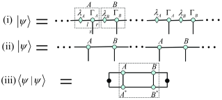
Figure 1: (color online) (i) Diagrammatic infinite matrix product state (iMPS) representation of a wavefunction $|\Psi\rangle$ having two-site translational invariance for infinite one-dimensional lattice systems. $\lambda_{A(B)}$ denoted by filled diamonds are a diagonal (singular value) matrix, respectively, depending on the $2i$-th ($A$) and $2i+1$-th ($B$) bonds. $\Gamma_{A(B)}$ indicated by filled circles are a three-index tensor for the $2i$-th and $2i+1$-th sites, respectively. $r$ and $l$ indicate the bond indices. (ii) A compact form of the pictorial representation in (i), where $A$ and $B$ (filled circles) by absorbing $\lambda$ into the tensors $\Gamma$ (indicated by the dashed-line box in (i)) present the lattice sites. (iii) The norm $\langle\Psi|\Psi\rangle$ of a given state $|\Psi\rangle$ in (i). The black dots indicate the left and right dominant eigenvectors that can be determined for the dominant eigenvalue of the transfer matrix $T$. The transfer matrix $T$ is obtained by the contraction on the tensors $A$, $A^{*}$, $B$, and $B^{*}$ in the dashed-line box.

For an infinite one-dimensional lattice system, a state can be written as Vidal2 ; Wolf

$$|\Psi\rangle=\sum_{\{S\}}\sum_{\{\alpha\}}\cdots\lambda^{[i]}_{\alpha_{i}}\Gamma^{[i]}_{\alpha_{i},s_{i},\alpha_{i+1}}\lambda^{[i+1]}_{\alpha_{i+1}}\Gamma^{[i+1]}_{\alpha_{i+1},s_{i+1},\alpha_{i+2}}\lambda^{[i+2]}_{\alpha_{i+2}}\cdots$$

$$~{}\hskip 56.9055pt\times|\cdots S_{i-1}S_{i}S_{i+1}\cdots\rangle,$$ (1)

where $|S_{i}\rangle$ denote a basis of the local Hilbert space at the site $i$, the elements of a diagonal matrix $\lambda^{[i]}_{\alpha_{i}}$ are the Schmidt decomposition coefficients of the bipartition between the semi-infinite chains $L(-\infty,...,i)$ and $R(i+1,...,\infty)$, and $\Gamma^{[i]}_{\alpha_{i},S_{i},\alpha_{i+1}}$ are a three-index tensor. The physical indices $S_{i}$ take the value $1,\cdots,d$ with the local Hilbert space dimension $d$ at the site $i$. The bond indices $\alpha_{i}$ take the value $1,\cdots,\chi$ with the truncation dimension of the local Hilbert space at the site $i$. The bond indices connect the tensors $\Gamma$ in the nearest neighbor sites. Such a representation in Eq. (1) is called the iMPS representation Vidal2 . If a system Hamiltonian has a translational invariance, one can introduce a translational invariant iMPS representation for a state. Practically, for instance, for a two-site translational invariance, the state can be reexpressed in terms of only the three-index tensors $\Gamma_{A(B)}$ and the two diagonal matrices $\lambda_{A(B)}$ for the even (odd) sites Li , where $\{\Gamma,\lambda\}$ are in the canonical form, i.e.,

$$|\Psi\rangle=\sum_{\{S\}}\sum_{\{l,r\}}\cdots\lambda_{A}\Gamma_{A}\lambda_{B}\Gamma_{B}\lambda_{A}\cdots|\cdots S_{i-1}S_{i}S_{i+1}\cdots\rangle,$$ (2)

where $l$ and $r$ are the left and right bond indices, respectively. In Fig. 1 (i), a state $|\Psi\rangle$ with a two-site translational invariance is pictorially displayed in the iMPS representation for infinite one-dimensional lattice systems. In a more compact form, further, the quantum state can be reexpressed as the state in Fig. 1 (ii) by absorbing the diagonal matrices $\lambda$ into the tensors $\Gamma$.

Once a random initial state $|\Psi(0)\rangle$ is prepared in the iMPS representation, one may employ the iTEBD algorithm Vidal2 to calculate a groundstate wavefunction numerically. For instance, if a system Hamiltonian is translational invariant and the interaction between spins consists of the nearest-neighbor interactions, i.e., the Hamiltonian can be expressed by $H=\sum_{i}h^{[i,i+1]}$, where $h^{[i,i+1]}$ is the nearest-neighbor two-body Hamiltonian density, a groundstate wavefunction of the system can be expressed in the form in Eq. (2). The imaginary time evolution of the prepared initial state $|\Psi(0)\rangle$, i.e.,

$$|\Psi(\tau)\rangle=\frac{\exp[-H\tau]|\Psi(0)\rangle}{||\exp[-H\tau]|\Psi(0)\rangle||},$$ (3)

leads to a groundstate of the system for a large enough $\tau$. By using the Suzuki-Trotter decomposition suzuki , actually, the imaginary time evolution operator $U=\exp[-H\tau]$ can be reduced to a product of two-site evolution operators $U(i,i+1)$ that only acts on two successive sites $i$ and $i+1$. For the numerical imaginary time evolution operation, the continuous time evolution can be approximately realized by a sequence of the time slice evolution gates $U(i,i+1)=\exp\left[-h^{[i,i+1]}\delta\tau\right]$ for the imaginary time slice $\delta\tau=\tau/n\ll 1$. A time-slice evolution gate operation contracts $\Gamma_{A}$, $\Gamma_{B}$, one $\lambda_{A}$, two $\lambda_{B}$, and the evolution operator $U(i,i+1)=\exp\left[-h^{[i,i+1]}\delta\tau\right]$. In order to recover the evolved state in the iMPS representation, a singular value decomposition (SVD) is performed and the $\chi$ largest singular values are obtained. From the SVD, the new tensors $\Gamma_{A}$, $\Gamma_{B}$, and $\lambda_{A}$ are generated. The latter is used to update the tensors $\lambda_{A}$ as the new one for all other sites. Similar contraction on the new tensors $\Gamma_{A}$, $\Gamma_{B}$, two new $\lambda_{A}$, one $\lambda_{B}$, and the evolution operator $U(i+1,i+2)=\exp\left[-h^{[i+1,i+2]}\right]$, and its SVD produce the updated $\Gamma_{A}$, $\Gamma_{B}$, and $\lambda_{B}$ for all other sites. After the time-slice evolution, then, all the tensors $\Gamma_{A}$, $\Gamma_{B}$, $\lambda_{A}$, and $\lambda_{B}$ are updated. This procedure is repeatedly performed until the system energy converges to a groundstate energy that yields a groundstate wavefunction in the iMPS representation. The normalization of the groundstate wavefunction is guaranteed by requiring the norm $\langle\Psi|\Psi\rangle=1$ in Fig. 1 (iii).

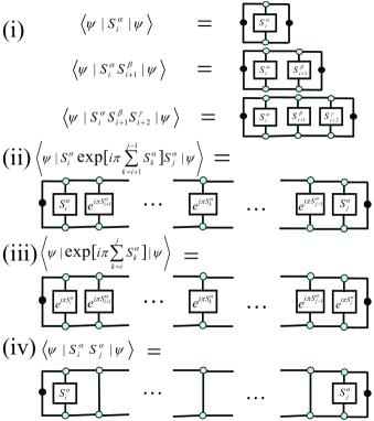
Figure 2: (color online) Diagrammatic representations of the expectation values in the iMPS representation. The black dots in left (right) side denote the dominant eigenvectors of the transfer matrix. In between a given wave function $|\Psi\rangle$ and its complex conjugate, each spin operator act on each site. (i) Local order computations including one, two, and three spins such as magnetization, dimer order, and chiral orders. Non-local correlations can also be calculated in the iMPS representation, e.g., (ii) string correlation $O^{\alpha}_{\textrm{S}}(i,j)=-\langle S^{\alpha}_{i}\exp[i\pi\sum_{k=i+1}^{j-1}S^{\alpha}_{k}]S^{\alpha}_{j}\rangle\,(\alpha\in\{x,y,z\})$, (iii) parity correlation $O^{\alpha}_{\textrm{P}}(i,j)=\langle\exp[i\pi\sum_{k=i}^{j}S^{\alpha}_{k}]\rangle$, and (iv) Néel correlation (two point spin correlation) $O^{\alpha}_{\textrm{N}}(i,j)=(-1)^{i-j}\langle S^{\alpha}_{i}S^{\alpha}_{j}\rangle.$

II.2 Non-local correlations

In principle, once one obtains a groundstate wavefunction, the expectation values of physical quantities can be calculated. In Fig. 2, we depict the diagrammatic iMPS representations for some examples of various expectation value calculations. Figure 2 (i) presents the computation of successive spin operators such as magnetization Zhao1 $\langle S^{\alpha}_{i}\rangle$, dimer order Yu $\langle S^{\alpha}_{i}S^{\beta}_{i+1}\rangle$, and chiral order Selinger ; Hikihara $\langle S^{\alpha}_{i}S^{\beta}_{i+1}S^{\gamma}_{i+2}\rangle$ ($\alpha,\beta,\gamma\in\{x,y,z\}$). On calculating the expectation values, each spin operator acting on a site is sandwiched between a given wave function $|\Psi\rangle$ and its complex conjugate. The left and right dominant eigenvectors of the transfer matrix denoted by the black dots act on the tensor, for instance, contracting the tensors $A$, $A^{*}$, (or $B$, $B^{*}$) and the local spin operator $S_{i}$ for $\langle S^{\alpha}_{i}\rangle$. This leads to the expectation value $\langle S^{\alpha}_{i}\rangle$.

This procedure can be simply expanded to the calculation of spin-spin correlations as well as non-local correlations. Examples are the string correlation ${\cal O}_{S}$ Nijs , the parity correlation ${\cal O}_{P}$ Hikihara , and the Néel correlation ${\cal O}_{N}$ Yu given by, respectively,

$${\cal O}^{\,\alpha}_{\textrm{S}}(i,j) = -\Bigg{\langle}S^{\alpha}_{i}\exp\Bigg{[}i\pi\sum_{k=i+1}^{j-1}S^{\alpha}_{k}\Bigg{]}S^{\alpha}_{j}\Bigg{\rangle},$$ (4a)

$${\cal O}^{\,\alpha}_{\textrm{P}}(i,j) = \Bigg{\langle}\exp\Bigg{[}i\pi\sum_{k=i}^{j}S^{\alpha}_{k}\Bigg{]}\Bigg{\rangle},$$ (4b)

$${\cal O}^{\,\alpha}_{\textrm{N}}(i,j) = (-1)^{i-j}\langle S^{\alpha}_{i}S^{\alpha}_{j}\rangle,$$ (4c)

where $i$ and $j$ denote the site locations in the lattice and then the lattice distance is $|i-j|$. Figures 2 (ii), (iii), and (iv) present the computation of the string, parity, and Néel correlations, respectively, in the iMPS representation. Note that, for the calculation of these correlations, the $(i-j)$ tensors are involved. For the parity correlation, the multi-site operator $\exp[i\pi\sum S^{\alpha}_{k}]$ acts on each site between the site $i$ and site $j$. For the string correlations, the spin operators $S_{i}$ and $S_{j}$ act on sites $i$ and $j$ while the multi-site operator $\exp[i\pi\sum S^{\alpha}_{k}]$ acts on the sites in between the sites $i$ and $j$. Compared to the string correlations, the Néel correlations can be calculated by replacing the multi-site operator $\exp[i\pi\sum S^{\alpha}_{k}]$ with the identity operator, i.e., $I_{i+1}\cdots I_{j-1}$ while the parity correlation can be obtained by expanding the multi-site spin operator to the both ends of the lattice distance. Then, it should be noted that, in principle, the iMPS representation allows to calculate any correlations in the limit of the infinite distance, i.e., $|i-j|\rightarrow\infty$. For numerical calculations, in order to obtain the correlations in the limit of the infinite distance, one can set a truncation error $\varepsilon$ rather than the lattice distance, i.e., ${\cal O}^{\,\alpha}(i,j)-{\cal O}^{\,\alpha}(i,j+1)<\varepsilon$. In this study, for instance, $\varepsilon=10^{-8}$ is chosen.

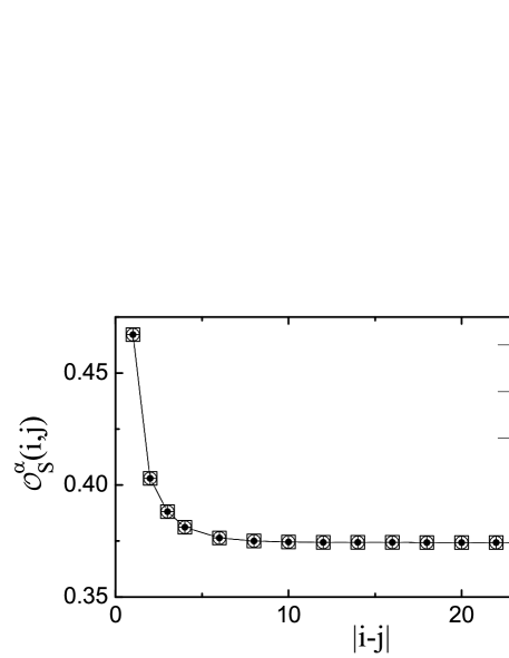
Figure 3: (color online) String correlation ${\cal O}^{\alpha}_{S}(i,j)$ for the Haldane spin-1 chain with truncation dimension $\chi=32$ in the iMPS representation. All components of the string correlations are well saturated to the value $O^{\alpha}_{S}=0.37434447$, which agrees very well with the result from the DMRG in Ref. White, .

As an example, for the spin-1 Haldane chain $H=\sum_{i}\mathbf{S}_{i}\cdot\mathbf{S}_{i+1}$, the exact-diagonalization calculations of a 14-site lattice have estimated ${\cal O}^{\,z}_{\textrm{S}}(\infty)\simeq 0.38$ Girvin . The DMRG methods have verified the existence of LRSO by estimating ${\cal O}^{\,z}_{\textrm{S}}(\infty)=0.37432509$ for the Haldane chain White . In Fig. 3, we plot the string correlation ${\cal O}^{\,\alpha}_{\textrm{S}}(i,j)$ as a function of the lattice distance $|i-j|$ with the truncation dimension $\chi=32$. It is shown clearly that the ${\cal O}^{\,\alpha}_{\textrm{S}}(i,j)$ starts to saturate around the lattice distance $|i-j|\simeq 10$ and ${\cal O}^{\,x}_{\textrm{S}}(i,j)={\cal O}^{\,y}_{\textrm{S}}(i,j)={\cal O}^{\,z}_{\textrm{S}}(i,j)$ for the Haldane chain. The saturated value of the string correlation from our iMPS representation approach is given as ${\cal O}^{\alpha}_{\textrm{S}}(\infty)=0.37434447$, which agrees very well with the value ${\cal O}^{z}_{\textrm{S}}(\infty)=0.37432509$ as well as the saturation behavior of the string correlations from the DMRG method in Fig. 5 of Ref. White, . As is well-known, further, the spin-1 AKLT model $H^{S=1}_{AKLT}=\sum_{i}[(1/2)\mathbf{S}_{i}\cdot\mathbf{S}_{i+1}+(1/6)(\mathbf{S}_{i}\cdot\mathbf{S}_{i+1})^{2}+1/3]$ is exactly solvable and the string order is given as the exact value $4/9$ Affleck ; Kolezhuk . In our iMPS representation, the value of the string order has been confirmed to be $4/9$ for the spin-1 AKLT model within the machine accuracy.

III spin-1 $XXZ$ Heisenberg chain

Spin-1 Heisenberg chains are one of the prototypical examples in understanding non-local correlations Alcaraz1 , i.e., string correlation. Then, to investigate non-local correlations in one-dimensional spin systems, we consider an infinite spin-1 $XXZ$ Heisenberg chain described by the Hamiltonian

$$H=J\sum^{\infty}_{i=-\infty}[S^{x}_{i}S^{x}_{i+1}+S^{y}_{i}S^{y}_{i+1}+\Delta S^{z}_{i}S^{z}_{i+1}],$$ (5)

where $S^{\alpha}_{i}(\alpha=x,y,z)$ are the spin-1 operators at the lattice site $i$, $J$ denotes the antiferromagnetic spin-exchange interaction between the nearest neighbor spins, and $\Delta$ is responsible for the anisotropy of the exchange interaction. This model has been intensively studied for a couple of decades Hatsugai ; Kennedy1 ; Kennedy2 ; Ueda ; wei ; Murashima ; Pan ; Alcaraz1 ; Botet ; Nomura ; Sakai ; Yajima ; Totsuka ; Tonegawa ; Yamanaka ; Boschi ; Ren ; Gu1 . The studies have shown that there are the four characteristic phases with respect to the anisotropic exchange interaction $\Delta$. If the anisotropic interaction is much smaller than $-1$, i.e., $\Delta\ll-1$, the Hamiltonian can be reduced to a spin-1 ferromagnetic Ising model $H\approx-\sum_{i}S^{z}_{i}S^{z}_{i+1}$ and the system is in the ferromagnetic phase. At $\Delta_{c1}=-1$, a first-order transition occurs between the ferromagnetic phase and the XY phase. If the anisotropic interaction is much greater than $1$, i.e., $\Delta\gg 1$, the Hamiltonian is reduced to a spin-1 antiferromagnetic Ising model $H\approx\sum_{i}S^{z}_{i}S^{z}_{i+1}$ and the system is in the antiferromagnetic (AF) phase. At $\Delta_{c3}=1.17\pm 0.02$, the Haldane-Néel phase transition occurs, which belongs to the two-dimensional Ising universality class Nomura ; Sakai . In between the two phase transition points $\Delta_{c1}<\Delta<\Delta_{c3}$, the XY-Haldane phase transition occurs, which has been thought to be a BKT transition at $\Delta_{c2}$ Alcaraz1 ; Botet ; Nomura ; Sakai .

As is well-known, many antiferromagnetic spin systems can be explored by the standard spin-spin correlations (Néel correlations) Yu . However, in the Haldane phase, the spin-spin correlations decay exponentially with a finite correlation length Lajko ; White ; Yamanaka ; Ueda and the Haldane gap exists. In this aspect, the Haldane phase can be considered as a disordered phase Charrier . Also, the XY phase is characterized by the power law decay of the spin-spin correlations (Néel correlations) Lajko with gapless excitations. Characterizing both the XY and Haldane phases therefore is a non-trivial task in the aspect of the spin-spin correlations. By investigating the spin correlations, the transition point $\Delta_{c2}$ has been estimated to be $0\lesssim\Delta_{c2}\lesssim 0.2$ from the exact numerical calculations and the finite-cell-scaling analysis Botet , $\Delta_{c2}=-0.01\pm 0.03$ from the phenomenological renormalization-group technique and the finite-size scaling analysis with 16 spin sites Sakai , and $\Delta_{c2}=0.068\pm 0.003$ from the criterion exponents of the spin correlations $\eta_{x}=1/4$ in the exact diagonalization method with 16 spin sites Yajima . Investigating the excitation gap, as the anisotropic interaction strength varies, is also a method to characterize the Haldane phase. By using the lowest-energy levels and finite-size scaling for energy gaps from the Lanczos method, the critical point has been conjectured to be at $\Delta_{c2}=0$ in Ref. Alcaraz1, . As an alternative way to characterize the Haldane phase, the string order arising due to the fully broken $Z_{2}\times Z_{2}$ hidden symmetry has been investigated Kennedy1 ; Kennedy2 . The XY-Haldane transition point has been estimated $\Delta_{c2}\sim 0$ by exploring the string correlations from a finite size analysis Alcaraz2 and by a finite-size scaling of the string order Ueda .

IV Behaviors of the string and Néel correlations in spin-1 XXZ chain

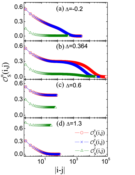
Figure 4: (color online) String correlations ${\cal O}^{\alpha}_{S}$ as a function of the lattice distance $|i-j|$ with the truncation dimension $\chi=32$ for various anisotropic interaction (a) $\Delta=-0.2$ and (b) $\Delta=0.364$ in the XY phase, (c) $\Delta=0.6$ in the Haldane phase, and (d) $\Delta=1.3$ in the Néel phase. In fact, for the truncation dimension $\chi=32$, the phase transition points are given as $\Delta_{c2}(\chi=32)=0.366$ and $\Delta_{c3}(\chi=32)=1.180$ in Fig. 6. It should be noted that, in the XY phase, the string correlations decay to zero with a unique two-step decaying behavior.

A non-vanishing correlation in the limit of the infinite lattice distance ($|i-j|\rightarrow\infty$), i.e., a long-rang order reveals that the system is in a ordered state. For the non-local correlations, the string and Néel orders are respectively defined by

$$O^{\,\alpha}_{\textrm{S}} = \lim_{|i-j|\rightarrow\infty}{\cal O}^{\,\alpha}_{\textrm{S}}(i,j),$$ (6a)

$$O^{\,\alpha}_{\textrm{N}} = \lim_{|i-j|\rightarrow\infty}{\cal O}^{\,\alpha}_{\textrm{N}}(i,j).$$ (6b)

For instance, the non-vanishing spin-spin (Néel) correlations for $|i-j|\rightarrow\infty$ indicate that the system is in an antiferromagnetic state. Also, the ground state in the Haldane phase is known to be characterized by the string order Kennedy2 . In the viewpoint of the string order, then, the Haldane phase could be an ordered phase. Further, if the string order plays a role as the order parameter for the Haldane phase, from the string order, the phase transition boundary from the Haldane phase to other phases can be captured. This view has been applied to the investigations of the Haldane phase of spin-1 systems Alcaraz2 ; Boschi ; Totsuka ; Tonegawa . By using numerical-diagonalization, however, available system sizes were too small to convince string order behaviors as an order parameter. Thus, in Ref. Ueda, , comparisons between the behaviors of the string and the Néel correlations from a finite size spin lattice (up to 300 sites), and their finite-size scaling behaviors have been used to capture the phase boundary. However, directly capturing the critical behavior of the string order near the transition point was quite difficult due to a very limited lattice size. Compared to such approaches, as discussed in Sec. II, the iMPS approach enables to explore the behaviors of the string order directly in the limit of the infinite lattice distance ($|i-j|\rightarrow\infty$).

In Fig. 4, we plot the string correlations ${\cal O}^{\,\alpha}_{S}(i,j)$ as a function of $|i-j|$ for various anisotropic interactions $\Delta$. In Figs. 4 (c) for the Haldane phase and (d) for the Néel (antiferromagnetic) phase, the string correlations show a logarithmical decaying to its saturated value or zero as the lattice distance $|i-j|$ increases up to a few hundreds. While, in the XY phase in Figs. 4 (a) and (b) , the string correlations show a unique two-step decaying to zero. As the lattice distance $|i-j|$ increases, that is, the string correlations undergo a decaying behavior for a few hundreds of the lattice distance, a saturation-like behavior for a few thousands of the lattice distance, and then eventually decaying again down to zero around a few tens of thousands. Hence, in contrast to the Haldane phase, there is no long-range string order in the XY phase. Also, it should be noted that, near the transition point in the XY phase in Fig. 4 (b), such saturation-like behaviors of the string correlations occur for a very wide range of the lattice distance from a few hundreds to a few thousands, i.e, roughly $10^{2}\lesssim|i-j|\lesssim 10^{4}$. While, away from the transition point in Fig. 4 (a), such saturation-like behaviors of the string correlations occur for a relatively narrow range of the lattice distance roughly $2\times 10^{2}\lesssim|i-j|\lesssim 10^{3}$. This saturation-like behavior of the string correlations makes the characterization of the Haldane phase quite difficult directly from a string order behavior in finite size systems. Indeed, compared to our iMPS results, a finite size system in the XY phase has given a finite value of the string correlation ${\cal O}^{\alpha}_{S}(i,j)$ within the limitation of the finite system sizes (up to 300 sites) Ueda .

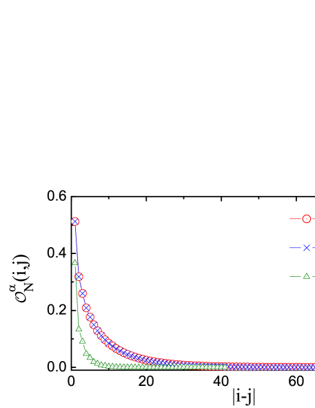
Figure 5: (color online) Néel correlations ${\cal O}^{\alpha}_{\textrm{N}}(i,j)$ in the Haldane phase ($\Delta=0.8$) with truncation dimension $\chi=32$. All components of the Néel correlations decay to zero exponentially. The transverse ($x$- and $y$- components) Néel correlations have a same value, i.e., ${\cal O}^{\,x}_{N}={\cal O}^{\,y}_{N}$.

In Fig. 5, a Néel correlation is displayed as a function of the lattice distance $|i-j|$. It is shown that, in the Haldane phase $\Delta=0.8$, the spin correlations (Néel correlations) decay exponentially to zero, which allows to characterize the phase transition from the Néel phase to the Haldane phase. As shown in Fig. 4 (d), in the Néel phase, in contrast to the $z$-component of the string correlations that survives for very large distances, the $x$- and $y$-components of the string correlations also decay exponentially to zero. Also, as shown in Fig. 4 (c), all the components of the string correlations in the Haldane phase have non-zero values in the limit of the infinite lattice distance. Then, alternatively, the $x$- and $y$-components of the string order make it possible to distinguish the Haldane phase from the Néel phase. Further, in the XY phase in Fig. 4 (b), all the components of the string order become zero with the unique two-step decaying behavior. As a consequence, the $x$- and $y$-components of the string order play a role of a true order parameter characterizing the Haldane phase from the XY phase and the Néel phase.

V Haldane phase and order parameter

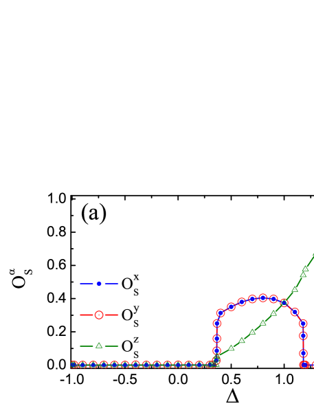
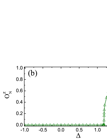
Figure 6: (color online) (a) String order parameters ${O}_{S}^{\,x,y}$ for the Haldane phase and (b) Néel order parameter ${O}^{\,z}_{N}$ for the Néel phase as a function of $\Delta$ with truncation dimension $\chi=32$. Note that the string order ${O}_{S}^{\,z}$ does not play a role as the order parameter to characterize the Haldane phase in (a). For this truncation dimension $\chi=32$, the system is in the XY phase for $-1<\Delta<0.366$, the Haldane phase for $0.366<\Delta<1.180$, and the Néel phase for $\Delta>1.180$. For the truncation dimension $\chi=32$, then, the transition points are $\Delta_{c2}=0.366$ and $\Delta_{c3}=1.180$.

As discussed in Sec. IV, the LRSOs can characterize the Haldane phase. In Fig. 6, we plot (a) the string orders ${\cal O}^{\,\alpha}_{S}$ and (b) the Néel order parameter ${O}^{\,z}_{N}$ as a function of the isotropic exchange interaction strength $\Delta$ for the truncation dimension $\chi=32$. It is shown that the ${O}^{\,x}_{S}={O}^{\,y}_{S}$ have non-zero values for $0.366<\Delta<1.180$, while the ${O}^{\,z}_{S}$ has a finite value for $\Delta>1.180$. The string orders become zero for $-1<\Delta<0.366$. Also, the Néel order parameter ${O}^{\,z}_{N}$ has a non-zero value for $\Delta>1.180$, which characterizes the Néel phase. This implies that the ${O}^{\,x}_{S}$ and ${O}^{\,y}_{S}$ are the order parameters for the Haldane phase. Then, the Haldane phase exists in the range of the anisotropic interaction strength $0.366<\Delta<1.180$, which implies $\Delta_{c2}=0.366$ and $\Delta_{c3}=1.180$ for the truncation dimension $\chi=32$. Thus, the XY phase occurs for $-1<\Delta<0.366$.

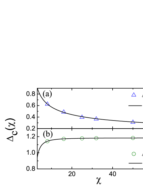
Figure 7: (color online) Phase transition points $\Delta_{c2}(\chi)$ and $\Delta_{c3}(\chi)$ as a function of the truncation dimension $\chi$. Here, the truncation dimensions are taken as $\chi=8$, $16$, $25$, $32$, $50$, and $64$. For the numerical extrapolation, the fitting functions are chosen as $\Delta_{c}(\chi)=a+b\chi^{-c}$, where $a$, $b$, and $c$ are a real number. A best numerical fitting gives (a) $a=0.015$, $b=1.366$, and $c=0.387$ for the XY-Haldane phase transition $\Delta_{c2}(\chi)$, and (b) $a=1.185$, $b=-1.748$, and $c=1.800$ for the Haldane-Néel phase transition $\Delta_{c3}(\chi)$. The estimated critical points in the thermodynamic limit are given by $\Delta_{c2}(\infty)=0.015$ for the XY-Haldane phase transition and $\Delta_{c3}(\infty)=1.185$ for the Haldane-Néel phase transition. The critical points agree well with the results from the previous studies Botet ; Sakai ; Yajima ; Ueda ; Nomura .

Actually, the transition points between the phases depend on the truncation dimension $\chi$, i.e., $\Delta_{c2}=\Delta_{c2}(\chi)$ and $\Delta_{c3}=\Delta_{c3}(\chi)$. As the truncation dimension $\chi$ increases from a lower truncation dimension (e.g., $\chi=8$), the phase transitions $\Delta_{c2}(\chi)$ and $\Delta_{c3}(\chi)$ occur starting at the lower and the higher values of $\Delta$’s, respectively. Then, the critical points $\Delta_{c2}(\infty)$ and $\Delta_{c3}(\infty)$ in the thermodynamic limit can be extrapolated to $\chi\rightarrow\infty$. In Fig. 7, we plot the transition points (a) $\Delta_{c2}(\chi)$ and (b) $\Delta_{c3}(\chi)$ as a function of the truncation dimension $\chi$. We employ an extrapolation function $\Delta(\chi)=a+b\chi^{-c}$, characterized by the fitting constants $a$, $b$, and $c$, which guarantees that $\Delta(\infty)$ becomes a finite value. The numerical fittings give, respectively, $a=0.015$, $b=1.366$ and $c=0.387$ for the phase transition between the XY and Haldane phases and $a=1.185$, $b=-1.748$, and $c=1.800$ for the phase transition from the Haldane phase to the Néel phase. In Fig. 7, in the limit of the infinite truncation dimension, i.e., $\chi\rightarrow\infty$, the fitting function are shown to saturate well to the extrapolated value $\Delta(\infty)=a$ which can be regarded as a critical point $\Delta_{c}=\Delta(\infty)$. As a result, our extrapolations give the critical points $\Delta_{c2}(\infty)=0.015$ and $\Delta_{c3}(\infty)=1.185$. Our critical points agree well with the results $\Delta_{c2}=0.068\pm 0.003$ from the exact diagonalization Yajima , $\Delta_{c2}=-0.01\pm 0.03$ from the phenomenological renormalization group with the finite-size scaling analysis Sakai , $\Delta_{c3}=1.17\pm 0.02$ Botet ; Sakai ; Nomura and $\Delta_{c3}=1.186$ Ueda from the DMRG.

VI XY phase

The XY phase is known to have a power-law decay of the spin-spin correlations with a gapless excitation. This implies that there exists no long-range order in the XY phase in the thermodynamic limit. Actually, in numerical approaches, directly characterizing a XY phase from a power-law decay of the spin-spin correlation is a non-trivial task. This may be the reason why a level spectroscopy of numerical approaches has been invented as a useful way to characterize the XY phase. However, directly detecting a vanishing excitation gap from numerical calculations near the transition point is also not a trivial work due to a very limited lattice size. As discussed in Sec. V, our iMPS approach has verified that the transverse string order parameter and the longitudinal Néel order parameter clearly characterize the Haldane phase and the Néel phase, respectively, in Figs. 6 (a) and (b). Obviously, the longitude Néel order and all the components of the string order become zero in the XY phase even for the finite truncation dimension $\chi$.

However, such vanishing behaviors of the long-range order parameters in the XY phase do not guarantee the existence of a XY phase in the iMPS representation. In this sense, it would be worthwhile to discuss a practical way to characterize the XY phase in the iMPS representation by defining a pseudo order parameter for a finite truncation dimension $\chi$. Then, some local or non-local properties of our iMPS groundstate will be introduced as indicators that can be used to distinguish a XY phase from other phases in the iMPS representation Zhou1 ; Wang1 .

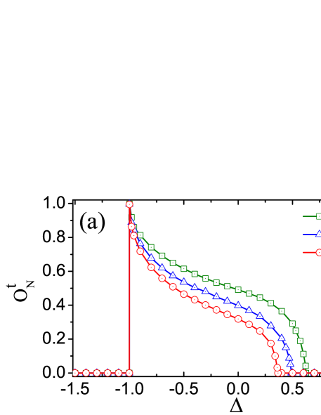
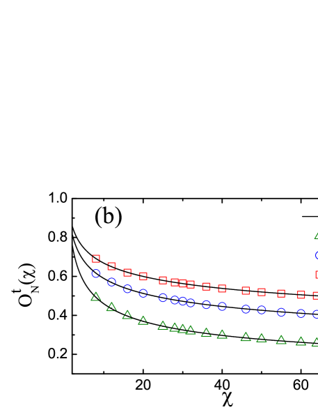
Figure 8: (color online) (a) Transverse Néel order ${O}^{\,t}_{N}={O}^{\,x}_{N}+{O}^{\,y}_{N}$ as a function of the anisotropic interaction $\Delta$ with for various values of the truncation dimension $\chi$. Note that, in the XY phase, the transverse Néel order is not zero for the finite truncation dimensions. (b) Transverse Néel order $O^{\,t}_{N}(\chi)$ as a function of the truncation dimension $\chi$ for $\Delta=0.0$, $-0.5$, and $-0.7$. For the numerical extrapolation, the fitting functions are chosen as ${O}^{\,t}_{N}(\chi)=a+b\chi^{-c}$, where $a$, $b$, and $c$ are a real number. A best fitting gives the fitting constants as (i) $a=0.446\times 10^{-4}$, $b=0.948$, and $c=0.315$ for $\Delta=0.0$, (ii) $a=3.643\times 10^{-3}$, $b=0.936$, and $c=0.203$ for $\Delta=-0.5$, and (iii) $a=0.897\times 10^{-4}$, $b=0.956$, and $c=0.156$ for $\Delta=-0.7$. These results show that, in the thermodynamic limit, the transverse Néel order does not exist in the XY phase, i.e., ${O}^{\,t}_{N}(\chi=\infty)=0$.

VI.1 Transverse Néel order for finite truncation dimensions

Let us consider the transverse Néel order in the XY phase. In Fig. 8 (a), we plot the transverse Néel order as a function of the anisotropic interaction strength $\Delta$ for various truncation dimensions. Here, the transverse Néel order is defined by the sum of the $x$- and $y$- components of the Néel order, ${O}^{\,t}_{N}(\chi)={O}^{\,x}_{N}(\chi)+{O}^{\,y}_{N}(\chi)$. It is shown that the transverse Néel order has a finite value in the XY phase. Actually, as the truncation dimension increases, as discussed in Sec. V, the interaction parameter range of the XY phase becomes narrower because the transition point $\Delta_{c2}(\chi)$ between the XY phase and the Haldane phase moves to a lower value for a higher truncation dimension. Note that, from the transverse Néel order, the transition points between the XY phase and the Haldane phase (non-zero values of the transverse Néel order) are the same with the values from the string order parameter, while the ferromagnetic-XY transition point does not move at $\Delta_{c1}=-1.0$. Thus, the non-vanishing transverse Néel order can be used as a pseudo order parameter characterizing the XY phase for a finite truncation dimension $\chi$.

Also, it should be noted that the overall amplitude of the transverse Néel order becomes smaller as the truncation dimension increases in Fig. 8 (a). In order to understand the transverse Néel order in the thermodynamic limit, i.e., $\chi\rightarrow\infty$, in Fig. 8 (b), we plot the transverse Néel order as a function of the truncation dimension $\chi$ for, as examples, three anisotropic interaction strengthes $\Delta=0$, $-0.5$, and $-0.7$. It is shown clearly that the transverse Néel order decreases as the truncation dimension increases. We perform an extrapolation by especially introducing a power-law fitting function ${O}^{\,t}_{N}(\chi)=a+b\chi^{-c}$ with respect to the truncation dimension $\chi$. The numerical fittings give (i) $a=0.446\times 10^{-4}$, $b=0.948$ and $c=0.315$ for $\Delta=0$, (ii) $a=3.643\times 10^{-3}$, $b=0.936$ and $c=0.203$ for $\Delta=-0.5$, and (iii) $a=0.897\times 10^{-4}$, $b=0.956$ and $c=0.156$ for $\Delta=-0.7$. Hence, the extrapolated values of the transverse Néel order for $\chi\rightarrow\infty$ are given as ${O}^{\,t}_{N}(\infty)=0.446\times 10^{-4}$, $3.643\times 10^{-3}$, and $0.897\times 10^{-4}$ for $\Delta=0$, $-0.5$, and $-0.7$, respectively. This implies that, similar to the power-law decay of spin-spin correlations with respect to the lattice distance, the transverse Néel order follows a power-law decaying to zero with respect to the truncation dimension $\chi$. These results show that, in the XY phase, the transverse Néel order as well as the longitudinal one also becomes zero, ${O}^{\,\alpha}_{N}(\infty)=0$. As a consequence, both the string and the Néel long-range orders do not exist in the XY phase.

VI.2 Pseudo local order for finite truncation dimensions

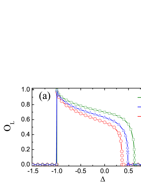
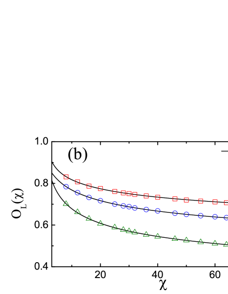
Figure 9: (color online) (a) Pseudo local order $O_{L}=\sqrt{\langle S_{x}\rangle^{2}+\langle S_{y}\rangle^{2}}$ for the XY phase as a function of the anisotropic interaction $\Delta$ for various values of the truncation dimension $\chi$. (b) Pseudo local order $O_{L}(\chi)$ as a function of the truncation dimension $\chi$ for $\Delta=0.0$, $-0.5$, and $-0.7$. By using the fitting function ${O}_{L}(\chi)=a\chi^{-b}(1+c\chi^{-1})$ with $a$, $b$, and $c$ being a real number, the numerical extrapolations give the fitting constants as (i) $a=0.980$, $b=0.159$, and $c=-0.028$ for $\Delta=0.0$, (ii) $a=0.998$, $b=0.108$, and $c=-0.120$ for $\Delta=-0.5$, and (iii) $a=0.967$, $b=0.075$, and $c=0.048$ for $\Delta=-0.7$.

Recently, a pseudo local order have been suggested for the XY phase in the iMPS representation in Ref. Wang1, . The local order can be defined as ${\cal O}_{L}=\sqrt{\langle S_{x}\rangle^{2}+\langle S_{y}\rangle^{2}}$. In Fig. 9 (a), we plot the pseudo local order ${\cal O}_{L}$ as a function of the anisotropic interaction strength $\Delta$ for various truncation dimensions. It is shown that the defined local order has a finite value in only the XY phase. Similar to the transverse Néel order, from the defined local order, the transition points between the XY phase and the Haldane phase (non-zero values of the defined local order) are detected at the same values from the string order parameter for the same truncation dimension $\chi$. Also, the ferromagnetic-XY transition points from the defined local order does not move at $\Delta_{c1}=-1.0$. Compared with the transverse Néel order, Fig. 9 (a) shows that the overall amplitude of the defined local order becomes smaller as the truncation dimension $\chi$ increases. In Fig. 9 (b), we plot the transverse Néel order as a function of the truncation dimension $\chi$ for, as examples, three anisotropic interaction strengthes $\Delta=0$, $-0.5$, and $-0.7$. It is shown clearly that the defined local order decreases as the truncation dimension increases. We perform an extrapolation with respect to the truncation dimension $\chi$ by using the same fitting function ${O}_{L}(\chi)=a\chi^{-b}(1+c\chi^{-1})$, with $a$, $b$, and $c$ being a real number, given in Ref. Wang1, . Figure 9 (b) shows the behaviors of the defined local order for the XY phase agree well with the results of spin-1/2 XXZ model in Ref. Wang1, . Hence, similar to the transverse Néel order, the defined local order can be used as a pseudo order parameter characterizing the XY phase for a finite truncation dimension $\chi$.

VII Entanglement entropy, Central charge, and universality class for phase transitions

Instead of using order parameters, recently, various types of quantum entanglement measures have been proposed as an indicator characterizing quantum phase transitions QPT ; Skr . One of successful measures is the von Neumann entropy for a bipartite system Osborne ; Chung ; Cho ; Vidal3 . Singular behaviors of bipartite entanglements for a pure state reveal quantum critical behaviors, which has been verified as being universal by extensive studies in many one-dimensional systems Osterloh ; entropy .

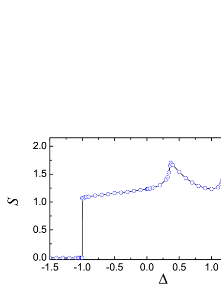
Figure 10: (color online) Von Neumann entropy as a function of the anisotropic interaction $\Delta$ for the truncation dimension $\chi=32$. The transition points are seen at $\Delta_{c1}=-1.0$, $\Delta_{c2}=0.366$, and $\Delta_{c3}=1.180$. This result is consistent with the phase transition points from the order parameters in Fig. 6.

Von Neumann entropy singularities.$-$ In the iMPS approach, the von Neuman entropy can be explored. Let us recall the diagonal matrix $\lambda$. As discussed in Sec. II, the elements of the diagonal matrix $\lambda^{[i]}_{\alpha_{i}}$ are the Schmidt decomposition coefficients of the bipartition between the semi-infinite chains $L(-\infty,...,i)$ and $R(i+1,...,\infty)$. This implies that Eq. (1) can be rewritten by $|\Psi\rangle=\sum^{\chi}_{\alpha=1}\lambda_{\alpha}|\psi^{L}_{\alpha}\rangle|\psi^{R}_{\alpha}\rangle$, where $|\psi^{L}_{\alpha}\rangle$ and $|\psi^{R}_{\alpha}\rangle$ are the Schmidt bases for the semi-infinite chains $L(-\infty,...,i)$ and $R(i+1,...,\infty)$, respectively. For the bipartition, then, the von Neumann entropy $S$ can be defined as Bennett $S=-{\rm Tr}[\varrho_{L}\log\varrho_{L}]=-{\rm Tr}[\varrho_{R}\log\varrho_{R}]$, where $\varrho_{L}={\rm Tr}_{R}\,\varrho$ and $\varrho_{R}={\rm Tr}_{L}\,\varrho$ are the reduced density matrices of the subsystems $L$ and $R$, respectively, with the density matrix $\varrho=|\Psi\rangle\langle\Psi|$. For the semi-infinite chains $L$ and $R$ in the iMPS representation, the von Neumann entropy $S$ is given by

$$S=-\sum_{\alpha=1}^{\chi}\lambda^{2}_{\alpha}\log\lambda^{2}_{\alpha}.$$ (7)

In Fig. 10, we plot the von Neumann entropy as a function of $\Delta$ for $\chi=32$. In the entropy, there are three singular points that consist of two local peaks ( $\Delta=0.366$ and $\Delta=1.180$, respectively ) and one discontinuous point ($\Delta=-1.0$). In fact, the singular points correspond to the transition points from the string order parameters and the Néel order parameter. It is shown that the von Neumann entropy captures the phase transitions. The discontinuity of the von Neumann entropy indicates that a discontinuous phase transition occurs between the Ferromagnetic phase and the XY phase. The two singular peaks show that the XY-Haldane phase transition and the Haldane-Néel phase transition belong to a continues phase transition. Especially, it should be noted that, in our iMPS representation, the von Neumann entropy can detect the BKT phase transition between the XY phase and the Haldane phase.

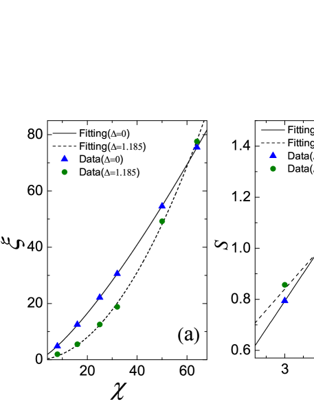
Figure 11: (color online) (a) Correlation length $\xi$ as a function of the truncation dimension $\chi$ at the critical points $\Delta_{c2}=0$ and $\Delta_{c3}=1.185$, respectively. The power curve fittings $\xi=\eta\chi^{\,\kappa}$ yields $\eta=0.330$ and $\kappa=1.306$ at $\Delta_{c2}=0$, and $\eta=0.023$ and $\kappa=1.955$ at $\Delta_{c3}=1.185$, respectively. (b) Scaling of the von Neumann entropy $S$ with respect to the truncation dimension $\chi$ at the critical points. From the fitting function $S(\chi)=a+b\log\chi$, the fitting constants are given as $a=0.139$ and $b=0.218$ at $\Delta_{c2}=0$, and $a=0.343$ and $b=0.166$ at $\Delta_{c3}=1.185$. From (i) $\kappa=1.306$ and $b=0.218$ at $\Delta_{c2}=0.0$, and (ii) $\kappa=1.955$ and $b=0.166$ at $\Delta_{c3}=1.185$ in (a) and (b), the central charges are determined as (i) $c=1.001$ and (ii) $c=0.509$, respectively.

Central charge and universality class.$-$ For one-dimensional quantum spin models, in general, the logarithmic scaling of von Neumann entropy was conformed to exhibit conformal invariance Korepin and the scaling is governed by a universal factor, i.e., a central charge of the associated conformal field theory. In fact, in the iMPS representation, a diverging entanglement at quantum criticality gives simple scaling relations for (i) the von Neumann entropy $S$ and (ii) a correlation length $\xi$ with respect to the truncation dimension $\chi$ as Korepin ; Tagliacozzo ; Pollmann

$$S \sim \frac{c\kappa}{6}\log\chi,$$ (8a)

$$\xi \sim \eta\chi^{\,\kappa},$$ (8b)

where $c$ is a central charge and $\kappa$ is a so-called finite-entanglement scaling exponent. Here, $\eta$ is a constant. By using Eqs. (8a) and (8b), then, a central charge can be obtained numerically at a critical point.

In the iMPS approach, the correlation length $\xi$ can be obtained from the transfer matrix $T$ defined in Fig. 1 (c). Actually, for a given $\chi$, the finite correlation length in the iMPS representation can be defined as $\xi(\chi)=1/\log{|\mu_{0}(\chi)/\mu_{1}(\chi)|}$, where the $\mu_{0}$ and $\mu_{1}$ are the largest and the second largest eigenvalues of the transfer matrix $T$, respectively. In Fig. 11, we plot (a) the correlation length $\xi$ and (b) the von Neumann entropy as a function of the truncation dimension $\chi$ at the critical points $\Delta_{c2}=0.0$ and $\Delta_{c3}=1.185$. Here, the truncation dimensions are taken as $\chi=8$, $16$, $25$, $32$, $50$, and $64$. It is shown that both the correlation length $\xi$ and the von Neumann entropy $S$ diverge as the truncation dimension $\chi$ increases. In order to obtain the central charges, we use the numerical fitting functions, i.e., $S(\chi)=a+b\log\chi$ and $\xi(\chi)=\eta\chi^{\,\kappa}$. From the numerical fittings of the von Neumann entropies $S$, the fitting constants are given as $a=0.139$ and $b=0.218$ for $\Delta_{c2}=0$, and $a=0.343$ and $b=0.166$ for $\Delta_{c3}=1.185$. Also, the power-law fittings on the correlation lengthes $\xi$ give the numerical fitting constants as $\kappa=1.306$ and $\eta=0.330$ for $\Delta_{c2}=0$, and $\kappa=1.955$ and $\eta=0.023$ for $\Delta_{c3}=1.185$. As a result, the central charges are given by $c=1.001$ for $\Delta_{c2}=0$ and $c=0.509$ for $\Delta_{c3}=1.185$. Our central charges are very close to the exact values $c=1$ and $c=0.5$, respectively. Therefore, the XY-Haldane phase transition at $\Delta_{c2}=0$ belongs to the Heisenberg universality class, while the Haldane-Néel phase transition at $\Delta_{c2}=1.185$ belongs to the two-dimensional classical Ising universality class.

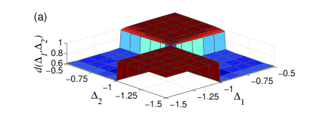
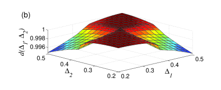
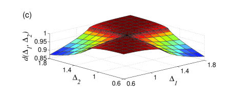
Figure 12: (color online) Fidelity per lattice site (FLS) $d(\Delta_{1},\Delta_{2})$ as a function of the anisotropic interactions $\Delta_{1}$ and $\Delta_{2}$ for the truncation dimension $\chi=32$. The pinch points are seen at (a) $\Delta=-1.0$, (b) $\Delta=0.366$, and (c) $\Delta=1.180$. These pinch points in the FLS are consistent with the phase transition points from the order parameters in Fig. 6. In (a) for the ferromagnetic-XY phase transition, the FLS discontinuity indicates that a first-order phase transition occurs at the transition point $\Delta=-1.0$. In (b) for the XY-Haldane phase transition and (c) for the Haldane-Néel phase transition, the continuous behaviors of the FLS across the pinch points implies that a continuous phase transition occurs at the transition points. It should be noted that the FLS captures a BKT phase transition between the XY and Haldane phases in (b).

VIII Fidelity per lattice site for phase transitions

For a quantum phase transition, the groundstate of a system undergoes a drastic change in its structure at a critical point Zanardi ; Zhou2 ; Rams . In fact, the groundstates in different phases should be orthogonal because the states are distinguishable in the thermodynamic limit Zhao1 ; Zhou2 . It implies that a comparison between quantum many-body states in different phases can signal quantum phase transitions regardless of what type of internal order exists in the states. Thus, as an alternative way to explore quantum phase transitions, the groundstate fidelity has been used in the last few years Zanardi ; Zhou2 ; Gu3 ; Rams ; Gong ; Zhao2 ; Mukherjee ; Liu ; Gu2 ; Xiao ; Chen . In contrast to quantum entanglement, the fidelity is a measure of similarity between two states. An abrupt change of the fidelity can then be expected across a critical point (in the thermodynamic limit). Based on understanding such a property of the groundstate fidelity near critical points, several measures have been suggested such as FLS Zhou2 , reduced fidelity Liu , fidelity susceptibility Gu3 , density-functional fidelity Gu2 , and operator fidelity Xiao . However, it is known that the fidelity susceptibility cannot detect a BKT type phase transition Ren ; Chen . Thus, the fidelity approaches have been thought to be a model-dependent indicator for quantum phase transitions. In order to show that a BKT type phase transition can be captured by the FLS approach, therefore, we discuss the FLS in the iMPS representation in this section.

Once one obtains the groundstate as a function of the anisotropic interaction strength $\Delta$, the groundstate fidelity is defined as $F(\Delta_{1},\Delta_{2})=|\langle\psi(\Delta_{2})|\psi(\Delta_{1})\rangle|$. Following Ref. Zhou3, , we define the groundstate FLS as

$$\ln d(\Delta_{1},\Delta_{2})\equiv\lim_{L\rightarrow\infty}\frac{\ln F(\Delta_{1},\Delta_{2})}{L},$$ (9)

where $L$ is the system size. The FLS is well defined in the thermodynamic limit even if $F(\Delta_{1},\Delta_{2})$ becomes trivially zero. From the fidelity $F(\Delta_{1},\Delta_{2})$, the FLS has several properties as (i) normalization $d(\Delta,\Delta)=1$, (ii) symmetry $d(\Delta_{1},\Delta_{2})=d(\Delta_{2},\Delta_{1})$, and (iii) range $0\leq d(\Delta_{1},\Delta_{2})\leq 1$. Within the iMPS approach, the FLS $d(\Delta_{1},\Delta_{2})$ Zhou3 is given by the largest eigenvalue $\mu_{0}$ of the transfer matrix $T$ up to the corrections that decay exponentially in the linear system size $L$. Then, for the infinite-size system, $d(\Delta_{1},\Delta_{2})=\mu_{0}$.

In Fig. 12, the groundstate FLSs $d$ are displayed as a function of the anisotropic interaction parameters ($\Delta_{1}$,$\Delta_{2}$) with the truncation dimension $\chi=32$. In the FLS surfaces, it is shown that there are three pinch points in the spin-1 XXZ model. Each pinch points correspond to the transition points identified from the order parameters. In Fig. 12 (a), the fidelity undergoes an abrupt change, which means that the first-order phase transition between the Ferromagnetic phase and the XY phase occurs at the pinch point. It is consistent with the discontinuous entropy in Fig. 10. In Fig. 12 (b), the pinch point corresponds to the XY-Haldane phase transition point. Contrasted to the fidelity susceptibility, the FLS is able to detect a BKT transition successfully, which is consistent with the result of our von Neumann entropy. Figure 12 (c) shows another continuous phase transition, i.e., the Haldane-Néel phase transition. Hence, it is shown that the FLS approach can be applied to characterize quantum phase transitions as a universal indicator Zhou2 ; Zhou3 .

IX Conclusions and remarks

We have investigated the string correlations in an infinite-size lattice of a spin-1 XXZ chain. In order to obtain a LRSO directly rather than an extrapolated string order in a finite-size system, the iMPS presentation has been employed and the groundstate wavefunction of the infinite lattice system has been numerically generated by the iTEBD algorithm. It was shown that the $x$- and $y$-components of the string correlations decay exponentially in the Néel phase, while they show a unique behavior of two-step decaying to zero within a relatively very large lattice distance in the XY phase. That is, there is no long-range transverse string order in the XY phase and the Néel phase. However, in the Haldane phase, the string correlations are saturated to finite values for a relatively smaller lattice distance, which shows clearly the existence of a LRSO. Consistently, the Néel order does not exit in both the XY phase and the Haldane phase. This result verifies that both the $x$- and $y$-components of the LRSO are the order parameters characterizing the Haldane phase. The estimated critical points agree well with the previous results as $\Delta_{c2}=0$ for the XY-Haldane phase transition and $\Delta_{c3}=1.185$ for the Haldane-Néel phase transition.

Further, the behaviors of the von Neumann entropy and the FLS have been discussed at the phase transition points. Both the von Neumann entropy and the FLS capture the corresponding phase transition points including the BKT point, which is consistent with the results from the string order parameter. Consequently, the von Neumann entropy as well as the fidelity approach based on the FLS can be applied to characterize quantum phase transitions as a universal phase transition indicator. Moreover, from a finite-entanglement scaling of the von Neumann entropy with respect to the truncation dimension, the central charges are obtained as $c\simeq 1$ at $\Delta_{c2}=0$ and $c\simeq 0.5$ at $\Delta_{c3}=1.185$, respectively, which shows the XY-Haldane phase transition at $\Delta_{c2}=0$ belongs to the Heisenberg universality class while the Haldane-Néel phase transition at $\Delta_{c2}=1.185$ belongs to the two-dimensional classical Ising universality class.

Contrary to other approaches, a feature of the iMPS approach is that, just from the iMPS groundstate, its critical behavior can be captured irrespective of whether a system has a finite excitation energy gap or not because, in principle, local and non-local order parameters can be calculated directly. Furthermore, von Neumann entropy and FLS can be used as a universal phase transition indicator for quantum phase transition in the iMPS representation. Hence, this iMPS approach would be widely applicable for capturing quantum critical phenomena in one-dimensional lattice many-body systems.

- (1) L. D. Landau and E. M. Lifshitz, Statistical Physicx (Pergamon, New York, 1958).
- (2) S. Sachdev, Quantum Phase Transitions (Cambridge University, Cambridge, 1999).
- (3) P. M. Chaikin and T. C. Lubensky, Pinciples of condensed matter physics (Cambridge University, Cambridge, 1995).
- (4) D. Belitz, T. R. Kirkpatrick, and T. Vojta, Phys. Rev. B 65, 165112 (2002).
- (5) Y. Hatsugai, J. Phys.: Condens Matter 19, 145209 (2007).
- (6) T. Kennedy, J. Phys.: Condens Matter 2, 5737 (1990).
- (7) T. Kennedy and H. Tasaki, Phys. Rev. B 45, 304 (1992).
- (8) F. C. Alcaraz and A. Moreo, Phys. Rev. B 46, 2896 (1992).
- (9) A. Kitazawa, K. Nomura, and K. Okamoto, Phys. Rev. Lett. 76, 4038 (1996).
- (10) U. Schollwöck, Th. Jolicoeur, and T. Garel, Phys. Rev. B 53, 3304 (1996).
- (11) V. O. Garlea, A. Zheludev, L.-P. Regnault, J.-H. Chung, Y. Qiu, M. Boehm, K. Habicht, and M. Meissner, Phys. Rev. Lett. 100, 037206 (2008).
- (12) D. Charrier, S. Capponi, M. Oshikawa, and P. Pujol, Phys. Rev. B 82, 075108 (2010).
- (13) H. J. Schulz, Phys. Rev. B 34, 6372 (1986).
- (14) F. C. Alcaraz and Y. Hatsugai, Phys. Rev. B 46, 13914 (1992).
- (15) H. Tasaki, Phys. Rev. Lett. 66, 798 (1991).
- (16) M. den Nijs and K. Rommelse, Phys. Rev. B 40, 4709 (1989).
- (17) I. Affleck, T. Kennedy, E. H. Lieb, and H. Tasaki, Phys. Rev. Lett. 59, 799 (1987).
- (18) A. K. Kolezhuk and U. Schollwöck, Phys. Rev. B 65, 100401 (2002).
- (19) F. D. M. Haldane, Phys. Lett. 93 A, 464 (1983); F. D. M. Haldane, Phys. Rev. Lett. 50, 1153 (1983).
- (20) W. J. L. Buyers, R. M. Morra, R. L. Armstrong, M. J. Hogan, P. Gerlach, and K. Hirakawa, Phys. Rev. Lett. 56, 371 (1986).
- (21) K. Katsumata, H. Hori, T. Takeuchi, M. Date, A. Yamagishi, and J. P. Renard, Phys. Rev. Lett. 63, 86 (1989).
- (22) K. Hida, Phys. Rev. B 45, 2207 (1992).
- (23) S. Yamamoto, Phys. Rev. B 55, 3603 (1997).
- (24) F. Anfuso and A. Rosch, Phys. Rev. B 76, 085124 (2007).
- (25) S. R. White, Phys. Rev. B 53, 52 (1996).
- (26) D. G. Shelton, A. A. Nersesyan, and A. M. Tsvelik, Phys. Rev. B 53, 8521 (1996).
- (27) E. Berg, E. G. DallaTorre, T. Giamarchi, and E. Altman, Phys. Rev. B 77, 245119 (2008).
- (28) T. Sakai and M. Takahashi, J. Phys. Soc. Jpn. 59, 2688 (1990).
- (29) K. Nomura, Phys. Rev. B 40, 9142 (1989).
- (30) R. Botet and R. Jullien, Phys. Rev. B 27, 613 (1983).
- (31) M. Yajima and M. Takahashi, J. Phys. Soc. Jpn. 63, 3634 (1994).
- (32) M. Fannes, B. Nachtergaele, and R. F. Werner, Comm. Math. Phys, 144, 3 (1994); S. Östlund and S. Rommer. Phys. Rev. Lett. 75, 3537 (1995).
- (33) H. Ueda, H. Nakano, and K. Kusakabe, Phys. Rev. B 78, 224402 (2008).
- (34) G. Vidal, Phys. Rev. Lett. 91, 147902 (2003).
- (35) G. Vidal, Phys. Rev. Lett. 98, 070201 (2007).
- (36) J.-H. Zhao, H.-L. Wang, B. Li, and H.-Q. Zhou, Phys. Rev. E 82, 061127 (2010).
- (37) B. Li, S. Y. Cho, H.-L. Wang, and B.-Q. Hu, J. Phys. A: Math. Theor. 44, 392002 (2011).
- (38) H.-L. Wang, J.-H. Zhao, B. Li, and H.-Q. Zhou, J. Stat. Mech., 10, L001 (2011).
- (39) V. Murg, F. Verstraete, and J. I. Cirac, Phys. Rev. A 75, 033605 (2007).
- (40) S. R. White, Phys. Rev. Lett. 69, 2863 (1992); S. R. White, Phys. Rev. B. 48, 10345 (1993); U. Schollwöck, Rev. Mod. Phys. 77, 259 (2005).
- (41) F. Verstraete and J. I. Cirac, arXiv:cond-mat/0407066.
- (42) M. M. Wolf, G. Ortiz, F. Verstraete, and J. I. Cirac, Phys. Rev. Lett. 97, 110403 (2006).
- (43) M. Suzuki, Phys. Lett. A 146, 319 (1990).
- (44) Y. Yu, G. Müller, and V. S. Viswanath, Phys. Rev. B 54, 9242(1996).
- (45) J. V. Selinger and R. L. B. Selinger, Phys. Rev. Lett. 76, 58 (1996).
- (46) T. Hikihara, M. Kaburagi, and H. Kawamura, Phys. Rev. B 63, 174430 (2001).
- (47) S. M. Girvin and D. P. Arovas, Phys. Scr. T 27, 156 (1989).
- (48) S. R. White and D. A. Huse, Phys. Rev. B 48, 3844 (1993).
- (49) M. Yamanaka, Y. Hatsugai, and M. Kohmoto, Phys. Rev. B 48, 9555 (1993).
- (50) C. D. E. Boschi and F. Ortolani, Eur. Phys. J. B 41, 503 (2004).
- (51) K. Totsuka, Y. Nishiyama, N. Hatano, and M. Suzuki, J. Phys.: Condens. Matter 7, 4895 (1995).
- (52) T. Tonegawa, T. Nakao, and M Kaburagi, J. Phys. Soc. Jpn. 65, 3317 (1996).
- (53) W. Chen, K. Hida, and B. C. Sanctuary, Phys. Rev. B 67, 104401 (2003).
- (54) T. Murashima, K. Hijii, K. Nomura, and T. Tonegawa, J. Phys. Soc. Jpn. 74, 1544 (2005).
- (55) S.-J. Gu, G.-S. Tian, and H.-Q. Lin, New J. Phys. 8, 61 (2006).
- (56) J. Ren and S. Zhu, Phys. Rev. A 79, 034302 (2009).
- (57) K.-K. Pan, Phys. Rev. B 79, 134414 (2009).
- (58) P. Lajkó, E. Carlon, H. Rieger, and F. Iglói, Phys. Rev. B 72, 094205 (2005).
- (59) H.-Q. Zhou, arXiv:cond-mat/0803.0585v1.
- (60) S. O. Skrøvseth, Phys. Rev. A 74, 022327 (2006).
- (61) G. Vidal, J. I. Latorre, E. Rico, and A. Kitaev, Phys. Rev. Lett. 90, 227902 (2003).
- (62) T. J. Osborne and M. A. Nielsen, Phys. Rev. A 66, 032110 (2002).
- (63) S. Y. Cho and R. H. McKenzie, Phys. Rev. A 73, 012109 (2006).
- (64) M.-H. Chung and D. P. Landau, Phys. Rev. B 83, 113104 (2011).
- (65) A. Osterloh, L. Amico, G. Falci, and R. Fazio, Nature (London) 416, 608 (2002).
- (66) L. Amico, R. Fazio, A. Osterloh, and V. Vedral, Rev. Mod. Phys. 80, 517 (2008).
- (67) C. H. Bennett, H. J. Bernstein, S. Popescu, and B. Schumacher, Phys. Rev. A 53, 2046 (1996).
- (68) V. E. Korepin, Phys. Rev. Lett. 92, 096402 (2004); P. Calabrese and J. Cardy, J. Stat. Mech.: Theory Exp., P06002 (2004).
- (69) L. Tagliacozzo, T. R. de Oliveira, S. Iblisdir, and J. I. Latorre, Phys. Rev. B 78, 024410 (2008).
- (70) F. Pollmann, S. Mukerjee, A. M. Turner, and J. E. Moore, Phys. Rev. Lett. 102, 255701 (2009).
- (71) P. Zanardi and N. Paunković, Phys. Rev. E 74, 031123 (2006);
- (72) H.-Q. Zhou and J.P. Barjaktarevič, J. Phys. A: Math. Theor. 41, 412001 (2008). H.-Q. Zhou, J.-H. Zhao, and B. Li, J. Phys. A: Math. Theor. 41, 492002 (2008); H.-Q. Zhou, arXiv:0704.2945.
- (73) M. M. Rams and B. Damski, Phys. Rev. Lett. 106, 055701 (2011).
- (74) J.-H. Liu, Q.-Q. Shi, J.-H. Zhao, and H.-Q. Zhou, arXiv:0905.3031; S.-H. Li, H.-L. Wang, Q.-Q. Shi, and H.-Q. Zhou, arXiv:1105.3008.
- (75) S. Yang, S.-J. Gu, C.-P. Sun, and H.-Q. Lin, Phys. Rev. A 78, 012304 (2008); S.-J. Gu, Int. J. Mod. Phys. B 24, 4371 (2010).
- (76) S.-J. Gu, Chin. Phys. Lett. 26, 026401 (2009).
- (77) X.-M. Lu, Z. Sun, X. Wang, and P. Zanardi, Phys. Rev. A 78, 032309 (2008); X. Wang, Z. Sun, and Z. D. Wang, Phys. Rev. A 79, 012105 (2009).
- (78) S. Chen, L. Wang, S. J. Gu, and Y. Wang, Phys. Rev. E 76, 061108 (2007).
- (79) V. Mukherjee and A. Dutta, Phys. Rev. B 83, 214302 (2011).
- (80) L. Gong and P. Tong, Phys. Rev. B 78, 115114 (2008).
- (81) J.-H. Zhao and H.-Q. Zhou, Phys. Rev. B 80, 014403 (2009).
- (82) H.-Q. Zhou, R. Orús, and G. Vidal, Phys. Rev. Lett. 100, 080601 (2008).