Cyber-Physical Systems under Attack – Part I:
Models and Fundamental Limitations

Attack Detection and Identification in Cyber-Physical Systems – Part I:
Models and Fundamental Limitations

Abstract

Cyber-physical systems integrate computation, communication, and physical capabilities to interact with the physical world and humans. Besides failures of components, cyber-physical systems are prone to malignant attacks, and specific analysis tools as well as monitoring mechanisms need to be developed to enforce system security and reliability. This paper proposes a unified framework to analyze the resilience of cyber-physical systems against attacks cast by an omniscient adversary. We model cyber-physical systems as linear descriptor systems, and attacks as exogenous unknown inputs. Despite its simplicity, our model captures various real-world cyber-physical systems, and it includes and generalizes many prototypical attacks, including stealth, (dynamic) false-data injection and replay attacks. First, we characterize fundamental limitations of static, dynamic, and active monitors for attack detection and identification. Second, we provide constructive algebraic conditions to cast undetectable and unidentifiable attacks. Third, by using the system interconnection structure, we describe graph-theoretic conditions for the existence of undetectable and unidentifiable attacks. Finally, we validate our findings through some illustrative examples with different cyber-physical systems, such as a municipal water supply network and two electrical power grids.

I Introduction

Cyber-physical systems arise from the tight integration of physical processes, computational resources, and communication capabilities. More precisely, processing units monitor and control physical processes by means of sensors and actuators networks. Examples of cyber-physical systems include transportation networks, power generation and distribution networks, water and gas distribution networks, and advanced communication systems. Due to the crucial role of cyber-physical systems in everyday life, cyber-physical security needs to be promptly addressed.

Besides failures and attacks on the physical infrastructure, cyber-physical systems are also prone to cyber attacks on their data management and communication layer. Recent studies and real-world incidents have demonstrated the inability of existing security methods to ensure a safe and reliable functionality of cyber-physical infrastructures against unforeseen failures and, possibly, external attacks [1, 2, 3, 4]. The protection of critical infrastructures is, as of today, one of the main focus of the Department of Homeland Security [5].

Concerns about security of control systems are not new, as the numerous manuscripts on systems fault detection, isolation, and recovery testify; see for example [6, 7]. Cyber-physical systems, however, suffer from specific vulnerabilities which do not affect classical control systems, and for which appropriate detection and identification techniques need to be developed. For instance, the reliance on communication networks and standard communication protocols to transmit measurements and control packets increases the possibility of intentional and worst-case (cyber) attacks against physical plants. On the other hand, information security methods, such as authentication, access control, message integrity, and cryptography methods, appear inadequate for a satisfactory protection of cyber-physical systems. Indeed, these security methods do not exploit the compatibility of the measurements with the underlying physical process and control mechanism, which are the ultimate objective of a protection scheme [8]. Moreover, such information security methods are not effective against insider attacks carried out by authorized entities, as in the famous Maroochy Water Breach case [3], and they also fail against attacks targeting directly the physical dynamics [9].

Related work. The analysis of vulnerabilities of cyber-physical systems to external attacks has received increasing attention in the last years. The general approach has been to study the effect of specific attacks against particular systems. For instance, in [10] deception and denial of service attacks against a networked control system are introduced, and, for the latter ones, a countermeasure based on semi-definite programming is proposed. Deception attacks refer to the possibility of compromising the integrity of control packets or measurements, and they are cast by altering the behavior of sensors and actuators. Denial of service attacks, instead, compromise the availability of resources by, for instance, jamming the communication channel. In [11] false data injection attacks against static state estimators are introduced. False data injection attacks are specific deception attacks in the context of static estimators. It is shown that undetectable false data injection attacks can be designed even when the attacker has limited resources. In a similar fashion, stealthy deception attacks against the Supervisory Control and Data Acquisition system are studied, among others, in [12, 13]. In [14] the effect of replay attacks on a control system is discussed. Replay attacks are cast by hijacking the sensors, recording the readings for a certain amount of time, and repeating such readings while injecting an exogenous signal into the system. It is shown that this type of attack can be detected by injecting a signal unknown to the attacker into the system. In [15] the effect of covert attacks against networked control systems is investigated. Specifically, a parameterized decoupling structure allows a covert agent to alter the behavior of the physical plant while remaining undetected from the original controller. In [16] a resilient control problem is studied, in which control packets transmitted over a network are corrupted by a human adversary. A receding-horizon Stackelberg control law is proposed to stabilize the control system despite the attack. Recently the problem of estimating the state of a linear system with corrupted measurements has been studied [17]. More precisely, the maximum number of faulty sensors that can be tolerated is characterized, and a decoding algorithm is proposed to detect corrupted measurements. Finally, security issues of some specific cyber-physical systems have received considerable attention, such as power networks [1, 2, 12, 18, 19, 20, 21, 22, 9], linear networks with misbehaving components [23, 24], and water networks [3, 13, 15, 25].

Contributions. The contributions of this paper are as follows. First, we describe a unified modeling framework for cyber-physical systems and attacks. Motivated by existing cyber-physical systems and proposed attack scenarios, we model a cyber-physical system under attack as a descriptor system subject to unknown inputs affecting the state and the measurements. For our model, we define the notions of detectability and identifiability of an attack by its effect on output measurements. Informed by the classic work on geometric control theory [26], our framework includes the deterministic static detection problem considered in [11, 12], and the prototypical deception and denial of service [10], stealth [18], (dynamic) false-data injection [27], replay [14], and covert attacks [15] as special cases. Second, we show the fundamental limitations of static, dynamic, and active detection and identification procedures. Specifically, we show that static detection procedures are unable to detect any attack affecting the dynamics, and that attacks corrupting the measurements can be easily designed to be undetectable. On the contrary, we show that undetectability in a dynamic setting is much harder to achieve for an attacker. Specifically, a cyber-physical attack is undetectable if and only if the attackers’ signal excites uniquely the zero dynamics of the input/output system. Additionally, we show that active monitors capable of injecting test signals are as powerful as dynamic (passive) monitors, since an attacker can design undetectable and unidentifiable attacks without knowing the signal injected by the monitor into the system. This analysis bring us also to the conclusion that undetectable attacks can be cast even without knowledge of system noise. Third, we provide a graph theoretic characterization of undetectable attacks. Specifically, we borrow some tools from the theory of structured systems, and we identify conditions on the system interconnection structure for the existence of undetectable attacks. These conditions are generic, in the sense that they hold for almost all numerical systems with the same structure, and they can be efficiently verified. As a complementary result, we extend a result of [28] on structural left-invertibility to regular descriptor systems. Fourth and finally, we illustrate the potential impact of our theoretical findings through compelling examples. In particular, we design (i) an undetectable state attack to destabilize the WSSC 3-machine 6-bus power system, (ii) an undetectable output attack for the IEEE 14 bus system, and (iii) an undetectable state and output attack to steal water from a reservoir of the EPANET network model 3. Through these examples we show the advantages of dynamic monitors against static ones, and we provide insight on the design of attacks.

Paper organization. The remainder of the paper is organized as follows. Section II presents some examples of cyber-physical systems. Section III contains our models of cyber-physical systems, attacks, and monitors. Our main results are presented in Section IV and in Section V. In particular, in Section IV we describe the fundamental limitations of static, dynamic, and active detectors, and we provide constructive algebraic conditions for the existence of undetectable and unidentifiable attacks. In Section V, instead, we derive graph-theoretic conditions for the existence of undetectable and unidentifiable attacks. Finally, Section VI and Section VII contain, respectively, our illustrative examples and our conclusion.

II Examples of cyber-physical systems

We now motivate our study by introducing important cyber-physical systems requiring advanced security mechanisms.

II-A Power networks

Future power grids will combine physical dynamics with a sophisticated coordination infrastructure. The cyber-physical security of the grid has been identified as an issue of primary concern [1, 2], which has recently attracted the interest of the control and power systems communities, see [12, 18, 19, 20, 21, 22].

We adopt the small-signal version of the classical structure-preserving power network model; see [19, 20] for a detailed derivation from the full nonlinear structure-preserving power network model. Consider a connected power network consisting of $n$ generators $\{g_{1},\dots,g_{n}\}$ and $m$ load buses $\{b_{n+1},\dots,b_{n+m}\}$. The interconnection structure of the power network is encoded by a connected susceptance-weighted graph. The generators $g_{i}$ and buses $b_{i}$ are the vertex set of this graph, and the edges are the transmission lines $\{b_{i},b_{j}\}$ weighted by the susceptance between buses $b_{i}$ and $b_{j}$, as well as the connections $\{g_{i},b_{i}\}$ weighted by the transient susceptance between generator $g_{i}$ and its adjacent bus $b_{i}$. The Laplacian associated with the susceptance-weighted graph is the symmetric susceptance matrix $\mathcal{L}=\left[\begin{smallmatrix}{\mathcal{L}}_{\textup{gg}}&{\mathcal{L}}_{\textup{gl}}\\ {\mathcal{L}}_{\textup{lg}}&{\mathcal{L}}_{\textup{ll}}\end{smallmatrix}\right]\in\mathbb{R}^{(n+m)\times(n+m)}$, where the first $n$ rows are associated with the generators and the last $m$ rows correspond to the buses. The dynamic model of the power network is

$$\begin{bmatrix}I\!\!&0\!\!&0\\ 0\!\!&{M}_{\textup{g}}\!\!&0\\ 0\!\!&0\!\!&0\end{bmatrix}\begin{bmatrix}\dot{\delta}(t)\\ \dot{\omega}(t)\\ \dot{\theta}(t)\end{bmatrix}\!=\!-\begin{bmatrix}0\!\!&-I\!\!&0\\ {\mathcal{L}}_{\textup{gg}}\!\!&{D}_{\textup{g}}\!\!&{\mathcal{L}}_{\textup{gl}}\\ {\mathcal{L}}_{\textup{lg}}\!\!&0\!\!&{\mathcal{L}}_{\textup{ll}}\end{bmatrix}\!\!\begin{bmatrix}\delta(t)\\ \omega(t)\\ \theta(t)\end{bmatrix}\!+\!\begin{bmatrix}0\\ P_{\omega}(t)\\ P_{\theta}(t)\end{bmatrix}\!,$$ (1)

where $\delta(t)\in\mathbb{R}^{n}$ and $\omega(t)\in\mathbb{R}^{n}$ denote the generator rotor angles and frequencies, and $\theta(t)\in\mathbb{R}^{m}$ are the voltage angles at the buses. The terms ${M}_{\textup{g}}$ and $D_{\textup{g}}$ are the diagonal matrices of the generator inertial and damping coefficients, and the inputs $P_{\omega}(t)$ and $P_{\theta}(t)$ are due to known changes in mechanical input power to the generators or real power demand at the loads.

II-B Mass transport networks

Mass transport networks are prototypical examples of cyber-physical systems modeled by differential-algebraic equations, such as gas transmission and distribution networks [29], large-scale process engineering plants [30], and water networks. Examples of water networks include open channel flows [31] for irrigation purposes and municipal water networks [32, 33]. The vulnerability of open channel networks to cyber-physical attacks has been studied in [13, 15], and municipal water networks are also known to be susceptible to attacks on the hydraulics [3] and biochemical contamination threats [25].

We focus on the hydraulics of a municipal water distribution network, as modeled in [32, 33]. The water network can be modeled as a directed graph with node set consisting of reservoirs, junctions, and storage tanks, and with edge set given by pipes, pumps, and valves that are used to convey water from source points to consumers. The key variables are the pressure head $h_{i}$ at each node $i$ in the network as well as the flows $Q_{ij}$ from node $i$ to $j$. The hydraulic model governing the network dynamics includes constant reservoir heads, flow balance equations at junctions and tanks, and pressure difference equations along all edges:

$$\begin{split}\mbox{reservoir }i:&\quad h_{i}={h_{i}}^{\textup{reservoir}}=\text{constant}\,,\\ \mbox{junction }i:&\quad d_{i}=\sum\nolimits_{j\to i}\!Q_{ji}-\sum\nolimits_{i\to k}\!Q_{ik}\,,\\ \mbox{tank }i:&\quad A_{i}\dot{h}_{i}=\sum\nolimits_{j\to i}\!Q_{ji}-\sum\nolimits_{i\to k}\!Q_{ik}\,,\\ \mbox{pipe }(i,j):&\quad Q_{ij}=Q_{ij}(h_{i}-h_{j})\,,\\ \mbox{pump }(i,j):&\quad h_{j}-h_{i}=+{\Delta h_{ij}}^{\textup{pump}}=\text{constant}\,,\\ \mbox{valve }(i,j):&\quad h_{j}-h_{i}=-{\Delta h_{ij}}^{\textup{valve}}=\text{constant}\,.\end{split}$$ (2)

Here $d_{i}$ is the demand at junction $i$, $A_{i}$ is the (constant) cross-sectional area of storage tank $i$, and the notation “$j\to i$” denotes the set of nodes $j$ connected to node $i$. The flow $Q_{ij}$ depends on the pressure drop $h_{i}-h_{j}$ along pipe according to the Hazen-Williams equation $Q_{ij}(h_{i}-h_{j})=g_{ij}|h_{i}-h_{j}|^{1/1.85-1}\cdot(h_{i}-h_{j})$, where $g_{ij}>0$ is the pipe conductance.

Other interesting examples of cyber-physical systems captured by our modeling framework are sensor networks, dynamic Leontief models of multi-sector economies, mixed gas-power energy networks, and large-scale control systems.

III Mathematical Modeling Of Cyber-physical Systems, Monitors, and Attacks

In this section we model cyber-physical systems under attack as linear time-invariant descriptor systems subject to unknown inputs. This modeling framework is very general and includes most of the existing cyber-physical models, attacks, and fault scenarios. Indeed, as shown in Section II, many interesting real-world cyber-physical systems contain conserved physical quantities leading to differential-algebraic system descriptions, and, as we show later, most attack and fault scenarios can be modeled by additive inputs affecting the state and the measurements.

Model of cyber-physical systems under attack. We consider the linear time-invariant descriptor system

$$\begin{split}E\dot{x}(t)&=Ax(t)+Bu(t),\\ y(t)&=Cx(t)+Du(t),\end{split}$$ (3)

where $x(t)\in\mathbb{R}^{n}$, $y(t)\in\mathbb{R}^{p}$, $E\in\mathbb{R}^{n\times n}$, $A\in\mathbb{R}^{n\times n}$, $B\in\mathbb{R}^{n\times m}$, $C\in\mathbb{R}^{p\times n}$, and $D\in\mathbb{R}^{p\times m}$. Here the matrix $E$ is possibly singular, and the input terms $Bu(t)$ and $Du(t)$ are unknown signals describing disturbances affecting the plant. Besides reflecting the genuine failure of systems components, these disturbances model the effect of an attack against the cyber-physical system (see below for our attack model). For notational convenience and without affecting generality, we assume that each state and output variable can be independently compromised by an attacker. Thus, we let $B=\begin{bmatrix}I,0\end{bmatrix}$ and $D=\begin{bmatrix}0,I\end{bmatrix}$ be partitioned into identity and zero matrices of appropriate dimensions, and, accordingly, $u(t)=\begin{bmatrix}u_{x}(t)^{\mathsf{T}},u_{y}(t)^{\mathsf{T}}\end{bmatrix}^{\mathsf{T}}$. Hence, the attack $(Bu(t),Du(t))=(u_{x}(t),u_{y}(t))$ can be classified as state attack affecting the system dynamics and as output attack corrupting directly the measurements vector.

The attack signal $t\mapsto u(t)\in\mathbb{R}^{n+p}$ depends upon the specific attack strategy. In the presence of $k\in\mathbb{N}_{0}$, $k\leq n+p$, attackers indexed by the attack set $K\subseteq\{1,\dots,n+p\}$ only and all the entries $K$ of $u(t)$ are nonzero over time. To underline this sparsity relation, we sometimes use $u_{K}(t)$ to denote the attack mode, that is the subvector of $u(t)$ indexed by $K$. Accordingly, the pair $(B_{K},D_{K})$, where $B_{K}$ and $D_{K}$ are the submatrices of $B$ and $D$ with columns in $K$, to denote the attack signature. Hence, $Bu(t)=B_{K}u_{K}(t)$, and $Du(t)=D_{K}u_{K}(t)$. Since the matrix $E$ may be singular, we make the following assumptions on system (3):

1. the pair $(E,A)$ is regular, that is, $\textup{det}(sE-A)$ does not vanish identically,

2. the initial condition $x(0)\in\mathbb{R}^{n}$ is consistent, that is, $(Ax(0)+Bu(0))\perp\operatorname{Ker}(E^{\mathsf{T}})=0$; and

3. the input signal $u(t)$ is smooth.

The regularity assumption (A1) assures the existence of a unique solution $x(t)$ to (3). Assumptions (A2) and (A3) simplify the technical presentation in this paper since they guarantee smoothness of the state trajectory $x(t)$ and the measurements $y(t)$; see [34, Lemma 2.5] for further details. The degree of smoothness in assumption (A3) depends on the index of $(E,A)$, see [35, Theorem 2.42], and continuity of $u(t)$ is sufficient for the index-one examples presented in Section II. In Section IV-E we discuss the results in this paper if assumptions (A2) and (A3) are dropped.

Model of static, dynamic, and active monitors. A monitor is a pair $(\Phi,\gamma(t))$, where $\Phi\,:\,\Lambda\,\rightarrow\,\Psi$ is an algorithm, and $\gamma\,:\,\mathbb{R}\mapsto\mathbb{R}^{n+p}$ is a signal. In particular, $\Lambda$ is the algorithm input to be specified later, $\Psi=\{\psi_{1},\psi_{2}\}$, with $\psi_{1}\in\{\textup{True},\textup{False}\}$ and $\psi_{2}\subseteq\{1,\dots,n+p\}$, is the algorithm output, and $(B\gamma(t),D\gamma(t))$ is an auxiliary input injected by the monitor into the system (3). In this work we consider the following classes of monitors for the system (3).

Definition 1

(Static monitor) A static monitor is a monitor with $\gamma(t)=0\;\forall t\in\mathbb{R}_{\geq 0}$, and $\Lambda=\{C,y(t)\;\forall t\in\mathbb{N}\}$.

Note that static monitors do not exploit relations among measurements taken at different time instants. An example of static monitor is the bad data detector [36].

Definition 2

(Dynamic monitor) A dynamic monitor is a monitor with $\gamma(t)=0\;\forall t\in\mathbb{R}_{\geq 0}$, and $\Lambda=\{E,A,C,y(t)\;\forall t\in\mathbb{R}_{\geq 0}\}$.

Differently from static monitors, dynamic monitors have knowledge of the system dynamics generating $y(t)$ and may exploit temporal relations among different measurements. The filters defined in [21] are examples of dynamic monitors.

Definition 3

(Active monitor) An active monitor is a monitor with $\gamma(t)\neq 0$ for some $t\in\mathbb{R}_{\geq 0}$, and $\Lambda=\{E,A,C,y(t)\;\forall t\in\mathbb{R}_{\geq 0}\}$.

Active monitors are dynamic monitors with the ability of modifying the system dynamics through an input. An example of active monitor is presented in [14] to detect replay attacks. The objective of a monitor is twofold:

Definition 4

(Attack detection) A nonzero attack $(B_{K}u_{K}(t),D_{K}u_{K}(t))$ is detected by a monitor if $\psi_{1}=\textup{True}$.

Definition 5

(Attack identification) A nonzero attack $(B_{K}u_{K}(t),D_{K}u_{K}(t))$ is identified by a monitor if $\psi_{2}=K$.

An attack is called undetectable (respectively unidentifiable) by a monitor if it fails to be detected (respectively identified) by every monitor in the same class. Of course, an undetectable attack is also unidentifiable, since it cannot be distinguished from the zero attack. By extension, an attack set $K$ is undetectable (respectively unidentifiable) if there exists an undetectable (respectively unidentifiable) attack $(B_{K}u_{K},D_{K}u_{K})$.

Model of attacks. In this work we consider colluding omniscient attackers with the ability of altering the cyber-physical dynamics through exogenous inputs. In particular we let the attack $(Bu(t),Du(t))$ in (3) be designed based on knowledge of the system structure and parameters $E,A,C$, and the full state $x(t)$ at all times. Additionally, attackers have unlimited computation capabilities, and their objective is to disrupt the physical state or the measurements while avoiding detection.

Remark 1

(Existing attack strategies as subcases)

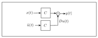
(a) Static stealth attack

(b) Replay attack

(d) Dynamic false data injection

Figure 1: A block diagram illustration of prototypical attacks is here reported. In Fig. 1(a) the attacker corrupts the measurements $y(t)$ with the signal $D_{K}u_{K}(t)\in\operatorname{Im}(C)$. Notice that in this attack the dynamics of the system are not considered. In Fig. 1(a) the attacker affects the output so that $y(t)=y(x(0),[\bar{u}_{K}^{\mathsf{T}}\;u_{K}^{\mathsf{T}}]^{\mathsf{T}},t)=y(\tilde{x}(0),0,t)$. The covert attack in Fig. 1(c) is a feedback version of the replay attack, and it can be explained analogously. In Fig. 1(d) the attack is such that the unstable pole $p$ is made unobservable.

​​​​​​
​​​​​​

(c) Covert attack

The following prototypical attacks can be modeled and analyzed through our theoretical framework:

1. stealth attacks defined in [18] correspond to output attacks compatible with the measurements equation;

2. replay attacks defined in [14] are state and output attacks which affect the system dynamics and reset the measurements;

3. covert attacks defined in [15] are closed-loop replay attacks, where the output attack is chosen to cancel out the effect on the measurements of the state attack; and

4. (dynamic) false-data injection attacks defined in [27] are output attacks rendering an unstable mode (if any) of the system unobservable.

A possible implementation of the above attacks in our model is illustrated in Fig. 1(a). $\square$

To conclude this section we remark that the examples presented in Section II are captured in our framework. In particular, classical power networks failures modeled by additive inputs include sudden change in the mechanical power input to generators, lines outage, and sensors failure; see [21] for a detailed discussion. Analogously, for a water network, faults modeled by additive inputs include leakages, variation in demand, and failures of pumps and sensors. Possible cyber-physical attacks in both power and water networks include comprising measurements [13, 12, 11] and attacks on the control architecture or the physical state itself [2, 9, 22, 3].

IV Limitations of static, dynamic and active monitors for detection and identification

The objective of this section is to highlight fundamental detection and identification limitations of static, dynamic, and active monitors. In particular, we show that the performance of widely used static monitors can be greatly improved by exploiting the system dynamics. On the other hand, the possibility of injecting monitoring signals does not improve the detection capabilities of a (passive) dynamic monitor.

Observe that a cyber-physical attack is undetectable if there exists a normal operating condition of the system under which the output would be the same as under the perturbation due to the attacker. Let $y(x_{0},u,t)$ be the output sequence generated from the initial state $x_{0}$ under the attack signal $u(t)$.

Lemma IV.1

(Undetectable attack) For the linear descriptor system (3), the attack $(B_{K}u_{K},D_{K}u_{K})$ is undetectable by a static monitor if and only if $y(x_{1},u_{K},t)=y(x_{2},0,t)$ for some initial condition $x_{1},x_{2}\in\mathbb{R}^{n}$ and for $t\in\mathbb{N}_{0}$. If the same holds for $t\in\mathbb{R}_{\geq 0}$, then the attack is also undetectable by a dynamic monitor.

Lemma IV.1 follows from the fact that our monitors are deterministic, so that $y(x_{1},u_{K},t)$ and $y(x_{2},0,t)$ lead to the same output $\psi_{1}$. A more general concern than detectability is identifiability of attackers, that is, the possibility to distinguish from measurements between the action of two distinct attacks. We quantify the strength of an attack through the cardinality of the attack set. Since an attacker can independently compromise any state variable or measurement, every subset of the states and measurements of fixed cardinality is a possible attack set.

Lemma IV.2

(Unidentifiable attack) For the linear descriptor system (3), the attack $(B_{K}u_{K},D_{K}u_{K})$ is unidentifiable by a static monitor if and only if $y(x_{1},u_{K},t)=y(x_{2},u_{R},t)$ for some initial condition $x_{1},x_{2}\in\mathbb{R}^{n}$, attack $(B_{R}u_{R},D_{R}u_{R})$ with $|R|\leq|K|$ and $R\neq{K}$, and for $t\in\mathbb{N}_{0}$. If the same holds for $t\in\mathbb{R}_{\geq 0}$, then the attack is also unidentifiable by a dynamic monitor.

Lemma IV.2 follows analogously to Lemma IV.1. We now elaborate on the above lemmas to derive fundamental detection and identification limitations for the considered monitors.

IV-A Fundamental limitations of static monitors

Following Lemma IV.1, an attack is undetectable by a static monitor if and only if, for all $t\in\mathbb{N}_{0}$, there exists a vector $\xi(t)$ such that $y(t)=C\xi(t)$. Notice that this condition is compatible with [11], where an attack is detected if and only if the residual $r(t)=y(t)-\tilde{C}\hat{x}(t)$ is nonzero for some $t\in\mathbb{N}_{0}$, where $\hat{x}(t)=C^{{\dagger}}y(t)$. In the following, let $\|v\|_{0}$ denote the number of nonzero components of the vector $v$.

Theorem IV.3

(Static detectability of cyber-physical attacks) For the cyber-physical descriptor system (3) and an attack set $K$, the following statements are equivalent:

1. the attack set $K$ is undetectable by a static monitor;

2. there exists an attack mode $u_{K}(t)$ satisfying, for some $x(t)$ and at every $t\in\mathbb{N}_{0}$,

   $$Cx(t)+D_{K}u_{K}(t)=0.$$ (4)

Moreover, there exists an attack set $K$, with $|K|=k\in\mathbb{N}_{0}$, undetectable by a static monitor if and only if there exist $x\in\mathbb{R}^{n}$ such that $\|Cx\|_{0}=k$.

Before presenting a proof of the above theorem, we highlight that a necessary and sufficient condition for the equation (4) to be satisfied is that $D_{K}u_{K}(t)=u_{y,K}(t)\in\operatorname{Im}(C)$ at all times $t\in\mathbb{N}_{0}$, where $u_{y,K}(t)$ is the vector of the last $p$ components of $u_{K}(t)$. Hence, statement (ii) in Theorem IV.3 implies that no state attack can be detected by a static detection procedure, and that an undetectable output attack exists if and only if $\operatorname{Im}(D_{K})\cap\operatorname{Im}(C)\neq\{0\}$.

Proof of Theorem IV.3:   As previously discussed, the attack $K$ is undetectable by a static monitor if and only if for each $t\in\mathbb{N}$ there exists $x(t)$, and $u_{K}(t)$ such that

$$r(t)=y(t)-CC^{\dagger}y(t)=(I-CC^{\dagger})\left(Cx(t)+D_{K}u_{K}(t)\right)$$

vanishes. Consequently, $r(t)=(I-CC^{\dagger})D_{K}u_{K}(t)$, and the attack set $K$ is undetectable if and only if $D_{K}u_{K}(t)\in\operatorname{Im}(C)$, which is equivalent to statement (ii). The last necessary and sufficient condition in the theorem follows from (ii), and the fact that every output variable can be attacked independently of each other since $D=\begin{bmatrix}0,I\end{bmatrix}$. ∎

We now focus on the static identification problem. Following Lemma IV.2, the following result can be asserted.

Theorem IV.4

(Static identification of cyber-physical attacks) For the cyber-physical descriptor system (3) and an attack set $K$, the following statements are equivalent:

1. the attack set $K$ is unidentifiable by a static monitor;

2. there exists an attack set $R$, with $|R|\leq|K|$ and $R\neq{K}$, and attack modes $u_{K}(t)$, $u_{R}(t)$ satisfying, for some $x(t)$ and at every $t\in\mathbb{N}_{0}$,

   $$Cx(t)+D_{K}\left(u_{K}(t)+u_{R}(t)\right)=0.$$

Moreover, there exists an attack set $K$, with $|K|=k\in\mathbb{N}_{0}$, unidentifiable by a static monitor if and only if there exists an attack set $\bar{K}$, with $|\bar{K}|\leq 2k$, which is undetectable by a static monitor.

Similar to the fundamental limitations of static detectability in Theorem IV.3, Theorem IV.4 implies that, for instance, state attacks cannot be identified and that an undetectable output attack of cardinality $k$ exists if and only if $\operatorname{Im}(D_{\bar{K}})\cap\operatorname{Im}(C)\neq\{0\}$, for some attack set $\bar{K}$ with $|\bar{K}|\leq 2k$.

Proof of Theorem IV.4:   Due to linearity of the system (3), the unidentifiability condition in Lemma IV.2 is equivalent to $y(x_{K}-x_{R},u_{K}-u_{R},t)=0$, for some initial conditions $x_{K}$, $x_{R}$, and attack modes $u_{K}(t)$, $u_{R}(t)$. The equivalence between statements (i) and (ii) follows. The last statement follows from Theorem IV.3. ∎

IV-B Fundamental limitations of dynamic monitors

As opposed to a static monitor, a dynamic monitor checks for the presence of attacks at every time $t\in\mathbb{R}_{\geq 0}$. Intuitively, a dynamic monitor is harder to mislead than a static monitor. The following theorem formalizes this expected result.

Theorem IV.5

(Dynamic detectability of cyber-physical attacks) For the cyber-physical descriptor system (3) and an attack set $K$, the following statements are equivalent:

1. the attack set $K$ is undetectable by a dynamic monitor;

2. there exists an attack mode $u_{K}(t)$ satisfying, for some $x(0)$ and for every $t\in\mathbb{R}_{\geq 0}$,

   $$E\dot{x}(t) =Ax(t)+B_{K}u_{K}(t)\,,$$

   $$0 =Cx(t)+D_{K}u_{K}(t)\,;$$

3. there exist $s\in\mathbb{C}$, $g\in\mathbb{R}^{|K|}$, and $x\in\mathbb{R}^{n}$, with $x\neq 0$, such that $(sE-A)x-B_{K}g=0$ and $Cx+D_{K}g=0$.

Moreover, there exists an attack set $K$, with $|K|=k$, undetectable by a dynamic monitor if and only if there exist $s\in\mathbb{C}$ and $x\in\mathbb{R}^{n}$ such that $\|(sE-A)x\|_{0}+\|Cx\|_{0}=k$.

Before proving Theorem IV.5, some comments are in order. First, differently from the static case, state attacks can be detected in the dynamic case. Second, in order to mislead a dynamic monitor an attacker needs to inject a signal which is consistent with the system dynamics at every instant of time. Hence, as opposed to the static case, the condition $D_{K}u_{K}(t)=u_{y,K}(t)\in\operatorname{Im}(C)$ needs to be satisfied for every $t\in\mathbb{R}_{\geq 0}$, and it is only necessary for the undetectability of an output attack. Indeed, for instance, state attacks can be detected even though they automatically satisfy the condition $D_{K}u_{K}(t)=0\in\operatorname{Im}(C)$. Third and finally, according to the last statement of Theorem IV.5, the existence of invariant zeros for the system $(E,A,B_{K},C,D_{K})$ is equivalent to the existence of undetectable attacks. As a consequence, a dynamic monitor performs better than a static monitor, while requiring, possibly, fewer measurements. We refer to Section VI-B for an illustrative example of this last statement.

Proof of Theorem IV.5:   By Lemma IV.1 and linearity of the system (7), the attack mode $u_{K}(t)$ is undetectable by a dynamic monitor if and only if there exists $x_{0}$ such that $y(x_{0},u_{K},t)=0$ for all $t\in\mathbb{R}_{\geq 0}$, that is, if and only if the system (3) features zero dynamics. Hence, statements (i) and (ii) are equivalent. For a linear descriptor system with smooth input and consistent initial condition, the existence of zero dynamics is equivalent to the existence of invariant zeros [34, Theorem 3.2 and Proposition 3.4]. The equivalence of statements (ii) and (iii) follows. The last statement follows from (iii), and the fact that $B=\begin{bmatrix}I,0\end{bmatrix}$ and $D=\begin{bmatrix}0,I\end{bmatrix}$. ∎

We now consider the identification problem.

Theorem IV.6

(Dynamic identifiability of cyber-physical attacks) For the cyber-physical descriptor system (3) and an attack set $K$, the following statements are equivalent:

1. the attack set $K$ is unidentifiable by a dynamic monitor;

2. there exists an attack set $R$, with $|R|\leq|K|$ and $R\neq{K}$, and attack modes $u_{K}(t)$, $u_{R}(t)$ satisfying, for some $x(0)$ and for every $t\in\mathbb{R}_{\geq 0}$,

   $$E\dot{x}(t) =Ax(t)+B_{K}u_{K}(t)+B_{R}u_{R}(t)\,,$$

   $$0 =Cx(t)+D_{K}u_{K}(t)+D_{R}u_{R}(t)\,;$$

3. there exists an attack set $R$, with $|R|\leq|K|$ and $R\neq{K}$, $s\in\mathbb{C}$, $g_{K}\in\mathbb{R}^{|K|}$, $g_{R}\in\mathbb{R}^{|R|}$, and $x\in\mathbb{R}^{n}$, with $x\neq 0$, such that $(sE-A)x-B_{K}g_{K}-B_{R}g_{R}=0$ and $Cx+D_{K}g_{K}+D_{R}g_{R}=0$.

Moreover, there exists an attack set $K$, with $|K|=k\in\mathbb{N}_{0}$, unidentifiable by a dynamic monitor if and only if there exists an attack set $\bar{K}$, with $|\bar{K}|\leq 2k$, which is undetectable by a dynamic monitor.

Proof:   Notice that, because of the linearity of the system (3), the unidentifiability condition in Lemma IV.2 is equivalent to the condition $y(x_{K}-x_{R},u_{K}-u_{R},t)=0$, for some initial conditions $x_{K}$, $x_{R}$, and attack modes $u_{K}(t)$, $u_{R}(t)$. The equivalence between statements (i) and (ii) follows. Finally, the last two statements follow from Theorem IV.5, and the fact that $B=\begin{bmatrix}I,0\end{bmatrix}$ and $D=\begin{bmatrix}0,I\end{bmatrix}$. ∎

In other words, the existence of an unidentifiable attack set $K$ of cardinality $k$ is equivalent to the existence of invariant zeros for the system $(E,A,B_{\bar{K}},C,D_{\bar{K}})$, for some attack set $\bar{K}$ with $|\bar{K}|\leq 2k$. We conclude this section with the following remarks. The existence condition in Theorem 3.4 is hard to verify because of its combinatorial complexity: in order to check if there exists an unidentifiable attack set $K$, with $|K|=k$, one needs to certify the absence of invariant zeros for all possible $2k$-dimensional attack sets. Thus, a conservative verification scheme requires $\binom{n+p}{2k}$ tests. In Section V we present intuitive graph-theoretic conditions for the existence of undetectable and unidentifiable attack sets for a given sparsity pattern of the system matrices and generic system parameters. Finally, Theorem IV.6 includes as a special case Proposition 4 in [17], which considers exclusively output attacks.

IV-C Fundamental limitations of active monitors

An active monitor uses a control signal (unknown to the attacker) to reveal the presence of attacks; see [14] for the case of replay attacks. In the presence of an active monitor with input signal $w(t)=[w_{x}^{\mathsf{T}}(t)\;w_{y}^{\mathsf{T}}(t)]^{\mathsf{T}}$, the system (3) reads as

$$\begin{split}E\dot{x}(t)&=Ax(t)+B_{K}u_{K}(t)+w_{x}(t),\\ y(t)&=Cx(t)+D_{K}u_{K}(t)+w_{y}(t).\end{split}$$

Although the attacker is unaware of the signal $w(t)$, active and dynamic monitors share the same limitations.

Theorem IV.7

(Limitations of active monitors) For the cyber-physical descriptor system (3), let $w(t)$ be an additive signal injected by an active monitor. The existence of undetectable (respectively unidentifiable) attacks does not depend upon the signal $w(t)$. Moreover, undetectable (respectively unidentifiable) attacks can be designed independently of $w(t)$.

Proof:

For the system (3), let $u(t)$ be the attack mode, and let $w(t)$ be the monitoring input. Let $y(x,u,w,t)$ denotes the output generated by the inputs $u(t)$ and $w(t)$ with initial condition $x=x_{1}+x_{2}$. Observe that, because of the linearity of (3), we have $y(x,u,w,t)=y(x_{1},u,0,t)+y(x_{2},0,w,t)$, with consistent initial conditions $x_{1}$ and $x_{2}$. Then, an attack $u(t)$ is undetectable if and only if $y(x,u,w,t)=y(\bar{x},0,w,t)$, or equivalently $y(x_{1},u,0,t)+y(x_{2},0,w,t)=y(\bar{x}_{1},0,0,t)+y(x_{2},0,w,t)$, for some initial conditions $x$ and $\bar{x}=\bar{x}_{1}+x_{2}$. The statement follows, since, from the equality above, the detectability of $u(t)$ does not depend upon $w(t)$. ∎

As a consequence of Theorem IV.7, the existence of undetectable attacks is independent of the presence of known control signals. Therefore, in a worst-case scenario, active monitors are as powerful as dynamic monitors. Since replay attacks are detectable by an active monitor [14], Theorem IV.7 shows that replay attacks are not worst-case attacks.

Remark 2

(Undetectable attacks in the presence of state and measurements noise) The input $w(t)$ in Theorem IV.7 may represent sensors and actuators noise. In this case, Theorem IV.7 states that the existence of undetectable attacks for a noise-free system implies the existence of undetectable attacks for the same system driven by noise. The converse does not hold, since attackers may remain undetected by injecting a signal compatible with the noise statistics. $\square$

IV-D Specific results for index-one singular systems

For many interesting real-world descriptor systems, including the examples in Section II-A and II-B, the algebraic system equations can be solved explicitly, and the descriptor system (3) can be reduced to a nonsingular state space system. For this reason, this section presents specific results for the case of index-one systems [37]. In this case, without loss of generality, we assume the system (3) to be written in the canonical form

$$\begin{split}\begin{bmatrix}E_{11}&0\\ 0&0\end{bmatrix}\begin{bmatrix}\dot{x}_{1}\\ \dot{x}_{2}\end{bmatrix}&=\begin{bmatrix}A_{11}&A_{12}\\ A_{21}&A_{22}\end{bmatrix}\begin{bmatrix}x_{1}\\ x_{2}\end{bmatrix}+\begin{bmatrix}B_{1}\\ B_{2}\end{bmatrix}u_{K}(t),\\ y(t)&=\begin{bmatrix}C_{1}&C_{2}\end{bmatrix}\begin{bmatrix}x_{1}\\ x_{2}\end{bmatrix}+D_{K}u_{K}(t),\end{split}$$ (5)

where $E_{11}$ is nonsingular and $A_{22}$ is nonsingular. Consequently, the state $x_{1}$ and $x_{2}$ are referred to as dynamic state and algebraic state, respectively. The algebraic state can be expressed via the dynamic state and the attack mode as

$$x_{2}(t)=-A_{22}^{-1}A_{21}x_{1}(t)-A_{22}^{-1}B_{2}u_{K}(t).$$ (6)

The elimination of the algebraic state $x_{2}$ in the descriptor system (5) leads to the nonsingular state space system

$$\dot{x}_{1}= \;\underbrace{E_{11}^{-1}\left(A_{11}-A_{12}A_{22}^{-1}A_{21}\right)}_{\tilde{A}}x_{1}(t)$$

$$\;+\underbrace{E_{11}^{-1}\left(B_{1}-A_{12}A_{22}^{-1}B_{2}\right)}_{\tilde{B}_{K}}u_{K}(t),$$ (7)

$$y(t)= \;\underbrace{\left(C_{1}-C_{2}A_{22}^{-1}A_{21}\right)}_{\tilde{C}}x_{1}(t)+\underbrace{\left(D_{K}-C_{2}A_{22}^{-1}B_{2}\right)}_{\tilde{D}_{K}}u_{K}(t).$$

This reduction of the algebraic states is known as Kron reduction in the literature on power networks and circuit theory [38]. Hence, we refer to (7) as the Kron-reduced system.

Clearly, for any state trajectory $x_{1}(t)$ of the Kron-reduced system (7), the corresponding state trajectory $[x_{1}^{\mathsf{T}}(t)\;x_{2}^{\mathsf{T}}(t)]^{\mathsf{T}}$ of the (non-reduced) cyber-physical descriptor system (3) can be recovered by identity (6) and given knowledge of the input $u_{K}(t)$. The following subtle issues are easily visible in the Kron-reduced system (6). First, a state attack affects directly the output $y(t)$, provided that $C_{2}A_{22}^{-1}B_{2}u_{K}(t)\neq 0$. Second, since the matrix $A_{22}^{-1}$ is generally fully populated, an attack on a single algebraic component can affect not only the locally attacked state or its vicinity but larger parts of the system.

According to the transformations in (7), for each attack set $K$, the attack signature $(B_{K},D_{K})$ is mapped to the corresponding signature $(\tilde{B}_{K},\tilde{D}_{K})$ in the Kron-reduced system. As an apparent disadvantage, the sparsity pattern of the original (non-reduced) cyber-physical descriptor system (3) is lost in the Kron-reduced representation (7), and so is, possibly, the physical interpretation of the state and the direct representation of system components. However, as we show in the following lemma, the notions of detectability and identifiability of an attack set $K$ defined for the original descriptor system (3) are equivalent for the Kron-reduced system (7). This property renders the low-dimensional and nonsingular Kron-reduced system (7) attractive from a computational point of view to design attack detection and identification monitors; see [39].

Lemma IV.8

(Equivalence of detectability and identifiability under Kron reduction) For the cyber-physical descriptor system (3), the attack set $K$ is detectable (respectively identifiable) if and only if it is detectable (respectively identifiable) for the associated Kron-reduced system (7).

Proof:

The lemma follows from the fact that the input and initial condition to output map for the system (3) coincides with the corresponding map for the Kron-reduced system (7) and equation (6). Indeed, according to Theorem IV.5, the attack set $K$ is undetectable if and only if there exist $s\in\mathbb{C}$, $g\in\mathbb{R}^{|K|}$, and $x=[x_{1}^{\mathsf{T}}\;x_{2}^{\mathsf{T}}]^{\mathsf{T}}\in\mathbb{R}^{n}$, with $x\neq 0$, such that

$$(sE-A)x-B_{K}g=0\mbox{ and }Cx+D_{K}g=0\,.$$

Equivalently, by eliminating the algebraic constraints as in (6), the attack set $K$ is undetectable if and only if the conditons

$$(sI-\tilde{A})x_{1}-\tilde{B}_{K}g=0\mbox{ and }\tilde{C}x_{1}+\tilde{D}_{K}g=0$$

are satisfied together with $x_{2}=-A_{22}^{-1}A_{21}x_{1}-A_{22}^{-1}B_{2}g$. Notice that the latter equation is always satisfied due to the consistency assumption (A2), and the equivalence of detectability of the attack set $K$ follows. The equivalence of attack identifiability follows by analogous arguments. ∎

IV-E Attack detection and identification in presence of inconsistent initial conditions and impulsive attack signals

We now discuss the case of non-smooth attack signal and inconsistent initial condition. If the consistency assumption (A3) is dropped, then discontinuities in the state $x(t\downarrow 0)$ may affect the measurements $y(t\downarrow 0)$. For instance for index-one systems, an inconsistent initial condition leads to an initial jump for the algebraic variable $x_{2}(t\downarrow 0)$ to obey equation (6). Consequently, the inconsistent initial value $[0^{\mathsf{T}}\;x_{2}(0)^{\mathsf{T}}]^{\mathsf{T}}\in\operatorname{Ker}(E)$ cannot be recovered through measurements.

Assumption (A4) requires the attack signal to be sufficiently smooth such that $x(t)$ and $y(t)$ are at least continuous. Suppose that assumption (A4) is dropped and the input $u(t)$ belongs to the class of impulsive smooth distributions $\mathcal{C}_{\textup{imp}}=\mathcal{C}_{\textup{smooth}}\cup\mathcal{C}_{\textup{p-imp}}$, that is, loosely speaking, the class of functions given by the linear combination of a smooth function on $\mathbb{R}_{\geq 0}$ (denoted by $\mathcal{C}_{\textup{smooth}}$) and Dirac impulses and their derivatives at $t=0$ (denoted by $\mathcal{C}_{\textup{p-imp}}$), see [34],[35, Section 2.4]. In this case, an attacker commanding an impulsive input $u(0)\in\mathcal{C}_{\textup{imp}}$ can reset the initial state $x(0)$ and, possibly, evade detection.

The discussion in the previous two paragraphs can be formalized as follows. Let $\mathcal{V}_{c}$ be the subspace of points $x_{0}\in\mathbb{R}^{n}$ of consistent initial conditions for which there exists an input $u\in\mathcal{C}^{m}_{\textup{smooth}}$ and a state trajectory $x\in\mathcal{C}^{n}_{\textup{smooth}}$ to the descriptor system (3) such that $y(t)=0$ for all $t\in\mathbb{R}_{\geq 0}$. Let $\mathcal{V}_{d}$ (respectively $\mathcal{W}$) be the subspace of points $x_{0}\in\mathbb{R}^{n}$ for which there exists an input $u\in\mathcal{C}^{n+p}_{\textup{imp}}$ (respectively $u\in\mathcal{C}^{n+p}_{\textup{p-imp}}$) and a state trajectory $x\in\mathcal{C}^{n}_{\textup{imp}}$ (respectively $x\in\mathcal{C}^{n}_{\textup{p-imp}}$) to the descriptor system (3) such that $y(t)=0$ for all $t\in\mathbb{R}_{\geq 0}$. The output-nulling subspace $\mathcal{V}_{d}$ can be decomposed as follows:

Lemma IV.9

(Decomposition of output-nulling space [34, Theorem 3.2 and Proposition 3.4])) $\mathcal{V}_{d}=\mathcal{V}_{c}+\mathcal{W}+\operatorname{Ker}(E)$.

In words, from an initial condition $x(0)\in\mathcal{V}_{d}$ the output can be nullified by a smooth input or by an impulsive input (with consistent or inconsistent initial conditions in $\operatorname{Ker}(E)$).

In this work we focus on the smooth output-nulling subspace $\mathcal{V}_{c}$, which is exactly space of zero dynamics identified in Theorems IV.5 and IV.6. Hence, by Lemma IV.9, for inconsistent initial conditions, the results presented in this section are valid only for strictly positive times $t>0$. On the other hand, if an attacker is capable of injecting impulsive signals, then it can avoid detection for initial conditions $x(0)\in\mathcal{W}$.

V Graph theoretic detectability conditions

In this section we characterize undetectable attacks against cyber-physical systems from a structural perspective. In particular we will derive detectability conditions based upon a connectivity property of a graph associated with the system. For ease of notation, we now drop the subscript $K$ from $B_{K}$, $D_{K}$, and $u_{K}(t)$.

V-A Preliminary notions

We start by recalling some useful facts about structured systems and structural properties [40, 26]. Let a structure matrix $[M]$ be a matrix in which each entry is either a fixed zero or an indeterminate parameter. The system

$$\begin{split}[E]\dot{x}(t)&=[A]x(t)+[B]u(t),\\ y(t)&=[C]x(t)+[D]u(t).\end{split}$$ (8)

is called structured system, and it is sometimes referred to with the tuple $([E],[A],[B],[C],[D])$ of structure matrices. A system $(E,A,B,C,D)$ is an admissible realization of $([E],[A],[B],[C],[D])$ if it can be obtained from the latter by fixing the indeterminate entries at some particular value. Two systems are structurally equivalent if they are both an admissible realization of the same structured system. Let $d$ be the number of indeterminate entries of a structured system altogether. By collecting the indeterminate parameters into a vector, an admissible realization is mapped to a point in the Euclidean space $\mathbb{R}^{d}$. A property which can be asserted on a dynamical system is called structural if, informally, it holds for almost all admissible realizations. To be more precise, we say that a property is structural if and only if the set of admissible realizations satisfying such property forms a dense subset of the parameters space. For instance, left-invertibility of a nonsingular system is a structural property with respect to $\mathbb{R}^{d}$ [41].

Consider the structured cyber-physical system (8). It is often the case that, for the tuple $(E,A,B,C,D)$ to be an admissible realization of (8), the numerical entries need to satisfy certain algebraic relations. For instance, for $(E,A,B,C,D)$ to be an admissible power network realization, the matrices $E$ and $A$ need to be of the form (1). Let $\mathbb{S}\subseteq\mathbb{R}^{d}$ be the admissible parameter space. We make the following assumption:

• the admissible parameters space $\mathbb{S}$ is a polytope of $\mathbb{R}^{d}$, that is, $\mathbb{S}=\{x\in\mathbb{R}^{d}\;:\;Mx\geq 0\}$ for some matrix $M$.

It should be noticed that assumption (A4) is automatically verified for the case of power networks [20, Lemma 3.1]. Unfortunately, if the admissible parameters space is a subset of $\mathbb{R}^{d}$, then classical structural system-theoretic results are, in general, not valid [40, Section 15].

We now define a mapping between dynamical systems in descriptor form and digraphs. Let ($[E]$,$[A]$,$[B]$,$[C]$,$[D]$) be a structured cyber-physical system under attack. We associate a directed graph $G=(\mathcal{V},\mathcal{E})$ with the tuple ($[E]$,$[A]$,$[B]$,$[C]$,$[D]$). The vertex set is $\mathcal{V}=\mathcal{U}\cup\mathcal{X}\cup\mathcal{Y}$, where $\mathcal{U}=\{u_{1},\dots,u_{m}\}$ is the set of input vertices, $\mathcal{X}=\{x_{1},\dots,x_{n}\}$ is the set of state vertices, and $\mathcal{Y}=\{y_{1},\dots,y_{p}\}$ is the set of output vertices. If $(i,j)$ denotes the edge from the vertex $i$ to the vertex $j$, then the edge set $\mathcal{E}$ is $\mathcal{E}_{[E]}\cup\mathcal{E}_{[A]}\cup\mathcal{E}_{[B]}\cup\mathcal{E}_{[C]}\cup\mathcal{E}_{[D]}$, with $\mathcal{E}_{[E]}=\{(x_{j},x_{i}):[E]_{ij}\neq 0\}$, $\mathcal{E}_{[A]}=\{(x_{j},x_{i}):[A]_{ij}\neq 0\}$, $\mathcal{E}_{[B]}=\{(u_{j},x_{i}):[B]_{ij}\neq 0\}$, $\mathcal{E}_{[C]}=\{(x_{j},y_{i}):[C]_{ij}\neq 0\}$, and $\mathcal{E}_{[D]}=\{(u_{j},y_{i}):[D]_{ij}\neq 0\}$. In the latter, for instance, the expression $[E]_{ij}\neq 0$ means that the $(i,j)$-th entry of $[E]$ is a free parameter.

Example 1

(Power network structural analysis)

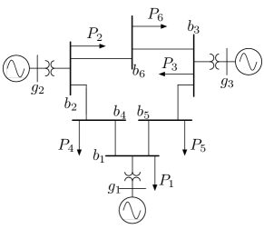
Figure 2: WSSC power system with $3$ generators and $6$ buses. The numerical value of the network parameters can be found in [19].

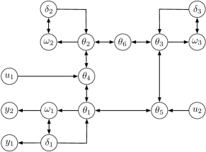
Figure 3: The digraph associated with the network in Fig. 2. The self-loops of the vertices $\{\delta_{1},\delta_{2},\delta_{3}\}$, $\{\omega_{1},\omega_{2},\omega_{3}\}$, and $\{\theta_{1},\dots,\theta_{6}\}$ are not drawn. The inputs $u_{1}$ and $u_{2}$ affect respectively the bus $b_{4}$ and the bus $b_{5}$. The measured variables are the rotor angle and frequency of the first generator.

Consider the power network illustrated in Fig. 2, where, being $e_{i}$ the $i$-th canonical vector, we take $[E]=\text{blkdiag}(1,1,1,M_{1},M_{2},M_{3},0,0,0,0,0,0)$, $[B]=[e_{8}\;e_{9}]$, $[C]=[e_{1}\;e_{4}]^{\mathsf{T}}$, $[D]=0$, and $[A]$ equal to

$$\left[\setcounter{MaxMatrixCols}{12}\begin{smallmatrix}0&0&0&1&0&0&0&0&0&0&0&0\\ 0&0&0&0&1&0&0&0&0&0&0&0\\ 0&0&0&0&0&1&0&0&0&0&0&0\\ a_{4,1}&0&0&a_{4,4}&0&0&a_{4,7}&0&0&0&0&0\\ 0&a_{5,2}&0&0&a_{5,5}&0&0&a_{5,8}&0&0&0&0\\ 0&0&a_{6,3}&0&0&a_{6,6}&0&0&a_{6,9}&0&0&0\\ a_{7,1}&0&0&0&0&0&a_{7,7}&0&0&a_{7,10}&a_{7,11}&0\\ 0&a_{8,2}&0&0&0&0&0&a_{8,8}&0&a_{8,10}&0&a_{8,12}\\ 0&0&a_{9,3}&0&0&0&0&0&a_{9,9}&0&a_{9,11}&a_{9,12}\\ 0&0&0&0&0&0&a_{10,7}&a_{10,8}&0&a_{10,10}&0&0\\ 0&0&0&0&0&0&a_{11,7}&0&a_{11,9}&0&a_{11,11}&0\\ 0&0&0&0&0&0&0&a_{12,8}&a_{12,9}&0&0&a_{12,12}\end{smallmatrix}\right]$$

The digraph associated with the structure matrices $([E],[A],[B],[C],[D])$ is shown in Fig. 3. $\square$

V-B Network vulnerability with known initial state

We derive graph-theoretic detectability conditions for two different scenarios. Recall from Lemma IV.1 that an attack $u(t)$ is undetectable if $y(x_{1},u,t)=y(x_{2},0,t)$ for some initial states $x_{1}$ and $x_{2}$. In this section, we assume that the system state is known at the failure initial time, so that an attack $u(t)$ is undetectable if $y(x_{0},u,t)=y(x_{0},0,t)$ for some system initial state $x_{0}$. The complementary case of unknown initial state is studied in Section V-C.

Consider the cyber-physical system described by the matrices $(E,A,B,C,D)$, and notice that, if the initial state is known, then the attack undetectability condition $y(x_{0},u,t)=y(x_{0},0,t)$ coincides with the system being not left-invertible. Recall that a subset $S\subseteq\mathbb{R}^{d}$ is an algebraic variety if it coincides with the locus of common zeros of a finite number of polynomials [26]. Consider the following observation.

Lemma V.1

(Polytopes and algebraic varieties) Let $S\subseteq\mathbb{R}^{d}$ be a polytope, and let $T\subseteq\mathbb{R}^{d}$ be an algebraic variety. Then, either $S\subseteq T$, or $S\setminus(S\cap T)$ is dense in $S$.

Proof:

Let $T\subseteq\mathbb{R}^{d}$ be the algebraic variety described by the locus of common zeros of the polynomials $\{\phi_{1}(x),\dots,\phi_{t}(x)\}$, with $t\in\mathbb{N}$, $t<\infty$. Let $P\subseteq\mathbb{R}^{d}$ be the smallest vector subspace containing the polytope $S$. Then $P\subseteq T$ if and only if every polynomial $\phi_{i}$ vanishes identically on $P$. Suppose that the polynomial $\phi_{i}$ does not vanish identically on $P$. Then, the set $T\cap P$ is contained in the algebraic variety $\{x\in P:\phi_{i}(x)=0\}$, and, therefore [26], the complement $P\setminus(P\cap T)$ is dense in $P$. By definition of a dense set, the set $S\setminus(S\cap T)$ is also dense in $S$. ∎

In Lemma V.1 interpret the polytope $S$ as the admissible parameters space of a structured cyber-physical system. Then we have shown that left-invertibility of a cyber-physical system is a structural property even when the admissible parameters space is a polytope of the whole parameters space. Consequently, given a structured cyber-physical system, either every admissible realization admits an undetectable attack, or there is no undetectable attack in almost all admissible realizations. Moreover, in order to show that almost all realizations have no undetectable attacks, it is sufficient to prove that this is the case for some specific admissible realizations. Before presenting our main result, we recall the following result. Let $\bar{E}$ and $\bar{A}$ be $N$-dimensional square matrices, and let $G(s\bar{E}-\bar{A})$ be the graph associated with the matrix $s\bar{E}-\bar{A}$ that consists of $N$ vertices, and an edge from vertex $j$ to $i$ if $\bar{A}_{ij}\neq 0$ or $\bar{E}_{ij}\neq 0$. The matrix $s[\bar{E}]-[\bar{A}]$ is said to be structurally degenerate if, for any admissible realization $\bar{E}$ (respectively $\bar{A}$) of $[\bar{E}]$ (respectively $[\bar{A}]$), the determinant $|s\bar{E}-\bar{A}|$ vanishes for all $s\in\mathbb{C}$. Recall the following definitions from [41]. For a given graph $G$, a path is a sequence of vertices where each vertex is connected to the following one in the sequence. A path is simple if every vertex on the path (except possibly the first and the last vertex) occurs only once. Two paths are disjoint if they consist of disjoint sets of vertices. A set of $l$ mutually disjoint and simple paths between two sets of vertices $S_{1}$ and $S_{2}$ is called a linking of size $l$ from $S_{1}$ to $S_{2}$. A simple path in which the first and the last vertex coincide is called cycle; a cycle family of size $l$ is a set of $l$ mutually disjoint cycles. The length of a cycle family equals the total number of edges in the family.

Theorem V.2

(Structural rank of a square matrix [42]) The structure $N$-dimensional matrix $s[\bar{E}]-[\bar{A}]$ is structurally degenerate if and only if there exists no cycle family of length $N$ in $G(s[\bar{E}]-[\bar{A}])$.

We are now able to state our main result on structural detectability.

Theorem V.3

(Structurally undetectable attack) Let the parameters space of the structured cyber-physical system $([E],[A],[B],[C],[D])$ define a polytope in $\mathbb{R}^{d}$ for some $d\in\mathbb{N}_{0}$. Assume that $s[E]-[A]$ is structurally non-degenerate. The system $([E],[A],[B],[C],[D])$ is structurally left-invertible if and only if there exists a linking of size $|\mathcal{U}|$ from $\mathcal{U}$ to $\mathcal{Y}$.

Theorem V.3 can be interpreted in the context of cyber-physical systems. Indeed, since $|sE-A|\neq 0$ by assumption (A1), and because of assumption (A4), Theorem V.3 states that there exists a structural undetectable attack if and only if there is no linking of size $|\mathcal{U}|$ from $\mathcal{U}$ to $\mathcal{Y}$, provided that the network state at the failure time is known.

Proof:

Because of Lemma V.1, we need to show that, if there are $|\mathcal{U}|$ disjoint paths from $\mathcal{U}$ to $\mathcal{Y}$, then there exists admissible left-invertible realizations. Conversely, if there are at most $|\mathcal{U}|-1$ disjoint paths from $\mathcal{U}$ to $\mathcal{Y}$, then every admissible realization is not left-invertible.

(If) Let $(E,A,B,C,D)$, with $|sE-A|\neq 0$, be an admissible realization, and suppose there exists a linking of size $|\mathcal{U}|$ from $\mathcal{U}$ to $\mathcal{Y}$. Without affecting generality, assume $|\mathcal{Y}|=|\mathcal{U}|$. For the left-invertibility property we need

$$\left|\begin{bmatrix}sE-A&-B\\ C&D\end{bmatrix}\right|=\left|sE-A\right|\left|D+C(sE-A)^{-1}B\right|\neq 0,$$

and hence we need $\left|D+C(sE-A)^{-1}B\right|\neq 0$. Notice that $D+C(sE-A)^{-1}B$ corresponds to the transfer matrix of the cyber-physical system. Since there are $|\mathcal{U}|$ independent paths from $\mathcal{U}$ to $\mathcal{Y}$, the matrix $D+C(sE-A)^{-1}B$ can be made nonsingular and diagonal by removing some connection lines from the network. In particular, for a given linking of size $|\mathcal{U}|$ from $\mathcal{U}$ to $\mathcal{Y}$, a nonsingular and diagonal transfer matrix is obtained by setting to zero the entries of $E$ and $A$ corresponding to the edges not in the linking. Then there exist admissible left-invertible realizations, and thus the system $([E],[A],[D],[C],[D])$ is structurally left-invertible.

(Only if) Take any subset of $|\mathcal{U}|$ output vertices, and let $|\mathcal{U}|-1$ be the maximum size of a linking from $\mathcal{U}$ to $\mathcal{Y}$. Let $[\bar{E}]$ and $[\bar{A}]$ be such that $s[\bar{E}]-[\bar{A}]=\left[\begin{smallmatrix}s[E]-[A]&[B]\\ [C]&[D]\end{smallmatrix}\right]$. Consider the previously defined graph $G(s[\bar{E}]-[\bar{A}])$, and notice that a path from $\mathcal{U}$ to $\mathcal{Y}$ in the digraph associated with the structured system corresponds, possibly after relabeling the output variables, to a cycle in involving input/output vertices in $G(s[\bar{E}]-[\bar{A}])$. Observe that there are only $|\mathcal{U}|-1$ such (disjoint) cycles. Hence, there is no cycle family of length $N$, being $N$ the size of $[\bar{A}]$, and the statement follows from Theorem V.2. ∎

To conclude this section, note that Theorem V.3 extends [28] to regular descriptor systems with constraints on parameters.

V-C Network vulnerability with unknown initial state

If the failure initial state is unknown, then a vulnerability is identified by the existence of a pair of initial conditions $x_{1}$ and $x_{2}$, and an attack $u(t)$ such that $y(x_{1},0,t)=y(x_{2},u,t)$, or, equivalently, by the existence of invariant zeros for the given cyber-physical system. We will now show that, provided that a cyber-physical system is left-invertible, its invariant zeros can be computed by simply looking at an associated nonsingular state space system. Let the state vector $x$ of the descriptor system (3) be partitioned as $[x_{1}^{\mathsf{T}}\;x_{2}^{\mathsf{T}}]^{\mathsf{T}}$, where $x_{1}$ corresponds to the dynamic variables. Let the network matrices $E$, $A$, $B$, $C$, and $D$ be partitioned accordingly, and assume, without loss of generality, that $E$ is given as $E=\textup{blkdiag}(E_{11},0)$, where $E_{11}$ is nonsingular. In this case, the descriptor model (3) reads as

$$\begin{split}E_{11}\dot{x}_{1}(t)&=A_{11}x_{1}(t)+B_{1}u(t)+A_{12}x_{2}(t)\,,\\ 0&=A_{21}x_{1}(t)+A_{22}x_{2}(t)+B_{2}u(t)\,,\\ y(t)&=C_{1}x_{1}(t)+C_{2}x_{2}(t)+Du(t)\,.\end{split}$$ (9)

Consider now the associated nonsingular state space system which is obtained by regarding $x_{2}(t)$ as an external input to the descriptor system (9) and the algebraic constraint as output:

$$\begin{split}\dot{x}_{1}(t)&=E_{11}^{-1}A_{11}x_{1}(t)+E_{11}^{-1}B_{1}u(t)+E_{11}^{-1}A_{12}x_{2}(t),\\ \tilde{y}(t)&=\begin{bmatrix}A_{21}\\ C_{1}\end{bmatrix}x_{1}(t)+\begin{bmatrix}A_{22}&B_{2}\\ C_{2}&D\end{bmatrix}\begin{bmatrix}x_{2}(t)\\ u(t)\end{bmatrix}\,.\end{split}$$ (10)

Theorem V.4

(Equivalence of invariant zeros) Consider the descriptor system (3) partitioned as in (9). Assume that, for the corresponding structured system $([E],[A],[B],[C],[D])$, there exists a linking of size $|\mathcal{U}|$ from $\mathcal{U}$ to $\mathcal{Y}$. Then, in almost all admissible realizations, the invariant zeros of the descriptor system (9) coincide with those of the associated nonsingular system (10).

Proof:

From Theorem V.3, the structured descriptor system $([E],[A],[B],[C],[D])$ is structurally left-invertible. Let $(E,A,B,C,D)$ be a left-invertible realization.

The proof now follows a procedure similar to [43, Proposition 8.4]. Let $s\in\mathbb{C}$ be an invariant zero for the nonsingular system (10) with state-zero direction $x_{1}\neq 0$ and input-zero direction $u$, that is

$$\begin{bmatrix}0\\ 0\\ 0\end{bmatrix}=\underbrace{\left[\begin{array}[]{c|cc}sI-E_{11}^{-1}A_{11}&-E_{11}A_{12}&-E_{11}^{-1}B_{1}\\ \hline\cr A_{21}&A_{22}&B_{2}\\ C_{1}&C_{2}&D\end{array}\right]}_{{P}_{\textup{nonsingular}}(s)}\begin{bmatrix}x_{1}\\ x_{2}\\ u\end{bmatrix}\,.$$

A multiplication of the above equation by $\textup{blkdiag}(E_{11},-I,I)$ and a re-partioning of the resulting matrix yields

$$\begin{bmatrix}0\\ 0\\ 0\end{bmatrix}=\underbrace{\left[\begin{array}[]{cc|c}sE_{11}-A_{11}&-A_{12}&-B_{1}\\ -A_{21}&-A_{22}&-B_{2}\\ \hline\cr C_{1}&C_{2}&D\end{array}\right]}_{{P}_{\textup{singular}}(s)}\begin{bmatrix}x_{1}\\ x_{2}\\ u\end{bmatrix}\,.$$ (11)

Since $x_{1}\neq 0$, we also have $x=[x_{1}^{\mathsf{T}}\;x_{2}^{\mathsf{T}}]^{\mathsf{T}}\neq 0$. Then, equation (11) implies that $s\in\mathbb{C}$ is an invariant zero of the descriptor system (9) with state-zero direction $x\neq 0$ and input-zero direction $u$. We conclude that the invariant zeros of the nonsingular system (10) are a subset of the zeros of the descriptor system (9). In order to continue, suppose that there is $s\in\mathbb{C}$ which is an invariant zero of the descriptor system (9) but not of the nonsingular system (10). Let $x=[x_{1}^{\mathsf{T}}\;x_{2}^{\mathsf{T}}]^{\mathsf{T}}\neq 0$ and $u$ be the associated state-zero and input-zero direction, respectively. Since $\operatorname{Ker}({P}_{\textup{singular}}(s))=\operatorname{Ker}({P}_{\textup{nonsingular}}(s))$ and $s$ is not a zero of the nonsingular system (10), it follows that $x_{1}=0$ and $x_{2}\neq 0$. Accordingly, we have that

$$\operatorname{Ker}\left(\begin{bmatrix}-A_{12}&-B_{1}\\ -A_{22}&-B_{2}\\ C_{2}&D\end{bmatrix}\right)\neq\{\emptyset\}\,.$$

It follows that the vector $[0^{\mathsf{T}}\;x_{2}^{\mathsf{T}}\;u^{\mathsf{T}}]^{\mathsf{T}}$ lies in the nullspace of ${P}_{\textup{singular}}(s)$ for each $s\in\mathbb{C}$, and thus the descriptor system (9) is not left-invertible. In conclusion, if the descriptor system (9) is left-invertible, then its invariant zeros coincide with those of the nonsingular system (10). ∎

It should be noticed that, because of Theorem V.4, under the assumption of left-invertibility, classical linear systems results can be used to investigate the presence of structural undetectable attacks in a cyber-physical system; see [41] for a survey of results on generic properties of linear systems.

VI Illustrative examples

VI-A An example of state attack against a power network

Consider the power network model analyzed in Example 1 and illustrated in Fig. 2, and let the variables $\theta_{4}$ and $\theta_{5}$ be affected, respectively, by the unknown and unmeasurable signals $u_{1}(t)$ and $u_{2}(t)$. Suppose that a monitoring unit is allowed to measure directly the state variables of the first generator, that is, $y_{1}(t)=\delta_{1}(t)$ and $y_{2}(t)=\omega_{1}(t)$.

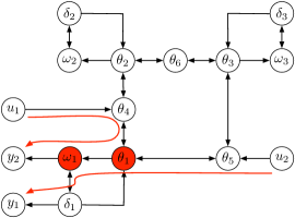
Figure 4: In the above network, there is no linking of size $2$ from the input to the output vertices. Indeed, the vertices $\theta_{1}$ and $\omega_{1}$ belong to every path from $\{u_{1},u_{2}\}$ to $\{y_{1},y_{2}\}$. Two input to output paths are depicted in red.

Notice from Fig. 4 that the maximum size of a linking from the failure to the output vertices is $1$, so that, by Theorem V.3, there exists a structural vulnerability. In other words, for every choice of the network matrices, there exist nonzero $u_{1}(t)$ and $u_{2}(t)$ that are not detectable through the measurements.

We now consider a numerical realization of this system. Let the input matrices be $B=[e_{8}\;e_{9}]$ and $D=[0\;0]^{\mathsf{T}}$, the measurement matrix be $C=[e_{1}\;e_{4}]^{\mathsf{T}}$, and the system matrix $A$ be as in equation (1) with $M_{g}=\text{blkdiag}(.125,.034,.016)$, $D_{g}=\text{blkdiag}(.125,.068,.048)$, and

$$\mathcal{L}=\!\left[\begin{smallmatrix}.058&0&0&-.058&0&0&0&0&0\\ 0&.063&0&0&-.063&0&0&0&0\\ 0&0&.059&0&0&-.059&0&0&0\\ -.058&0&0&.235&0&0&-.085&-.092&0\\ 0&-.063&0&0&.296&0&-.161&0&-.072\\ 0&0&-.059&0&0&.330&0&-.170&-.101\\ 0&0&0&-.085&-.161&0&.246&0&0\\ 0&0&0&-.092&0&-.170&0&.262&0\\ 0&0&0&0&-.072&-.101&0&0&.173\end{smallmatrix}\right].$$

Let $U_{1}(s)$ and $U_{2}(s)$ be the Laplace transform of the attack signals $u_{1}(t)$ and $u_{2}(t)$, and let

$$\begin{bmatrix}U_{1}(s)\\ U_{2}(s)\end{bmatrix}=\underbrace{\begin{bmatrix}\frac{-1.024s^{4}-5.121s^{3}-10.34s^{2}-9.584s-3.531}{s^{4}+5s^{3}+9.865s^{2}+9.173s+3.531}\\ 1\end{bmatrix}}_{\mathcal{N}(s)}\bar{U}(s),$$

for some arbitrary nonzero signal $\bar{U}(s)$. Then it can be verified that the failure cannot be detected through the measurements $y_{1}(t)$ and $y_{2}(t)$. In fact, $\mathcal{N}(s)$ coincides with the null space of the input/output transfer matrix. An example is in Fig. 5, where the second and the third generator are driven unstable by the attack, but yet the first generator does not deviate from the nominal operating condition.

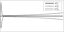
Figure 5: The velocities $\omega_{2}$ and $\omega_{3}$ are driven unstable by the signals $u_{1}(t)$ and $u_{2}(t)$, which are undetectable from the measurements of $\omega_{1}$ and $\delta_{1}$.

Suppose now that the rotor angle of the first generator and the voltage angle at the $6$-th bus are measured, that is, $C=[e_{1}\;e_{12}]^{\mathsf{T}}$. Then, there exists a linking of size $2$ from $\mathcal{U}$ to $\mathcal{Y}$, and the system $(E,A,B,C)$ is left-invertible. Following Theorem V.4, the invariant zeros of the power network can be computed by looking at its reduced system, and they are $-1.6864\pm 1.8070i$ and $-0.8136\pm 0.2258i$. Consequently, if the network state is unknown at the failure time, there exists vulnerabilities that an attacker may exploit to affect the network while remaining undetected. Finally, we remark that such state attacks are entirely realizable by cyber attacks [22].

VI-B An example of output attack against a power network

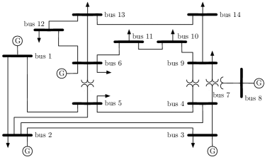
Figure 6: For the here represented IEEE 14 bus system, if the voltage angle of one bus is measured exactly, then a cyber attack against the measurements data is always detectable by our dynamic detection procedure. In contrary, as shown in [11], a cyber attack may remain undetected by a static procedure if it compromises as few as four measurements.

Let the IEEE 14 bus power network (Fig. 6) be modeled as a descriptor system as in Section II-A. Following [11], let the measurement matrix $C$ consist of the real power injections at all buses, of the real power flows of all branches, and of one rotor angle (or one bus angle). We assume that an attacker can compromise all the measurements, independently of each other, except for one referring to the rotor angle.

Let $k\in\mathbb{N}_{0}$ be the cardinality of the attack set. It is known that an attack undetectable to a static detector exists if $k\geq 4$ [11]. In other words, due to the sparsity pattern of $C$, there exists a signal $u_{K}(t)$, with (the same) four nonzero entries at all times, such that $Du_{K}(t)\in\operatorname{Im}(C)$ at all times. By Theorem IV.3 the attack set $K$ remains undetected by a Static Detector through the attack mode $u_{K}(t)$. On the other hand, following Theorem IV.5, it can be verified that, for the same output matrix $C$, and independent of the value of $k$, there exists no undetectable (output) attacks for a dynamic monitor.

It should be notice that this result relies on the fact that the rotor angle measurement is known to be correct, because, for instance, it is protected using sophisticated and costly security methods [1]. Since the state of the IEEE 14 bus system can be reconstructed by means of this measurement only (in a system theoretic sense, the system is observable by measuring one generator rotor angle), the output attack $Du(t)$ is easily identified as $Du(t)=y(t)-C\hat{x}(t)$, where $\hat{x}(t)=x(t)$ is the reconstructed system state at time $t$.

VI-C An example of state and output attack against a water supply network

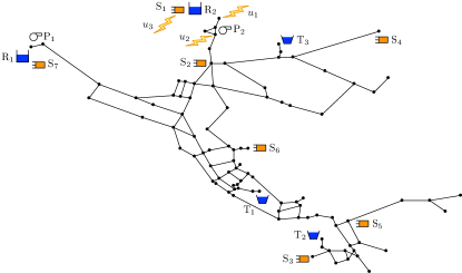
Figure 7: This figure shows the structure of the EPANET water supply network model # 3, which features $3$ tanks ($\text{T}_{1}$, $\text{T}_{2}$, $\text{T}_{3}$), $2$ reservoirs ($\text{R}_{1}$, $\text{R}_{2}$), $2$ pumps ($\text{P}_{1}$, $\text{P}_{2}$), $96$ junctions, and $119$ pipes. Seven pressure sensors ($\text{S}_{1},\dots,\text{S}_{7}$) have been installed to monitor the network functionalities. A cyber-physical attack to steal water from the reservoir $\text{R}_{2}$ is reported. Notice that the cyber-physical attack features two state attacks ($u_{1}$, $u_{2}$) and one output attack ($u_{3}$).

Consider the water supply network EPANET 3 linearized at a steady state with non-zero pressure drops [44]. The water network model as well as a possible cyber-physical attack are illustrated in Fig. 7. The considered cyber-physical attack aims at stealing water from the reservoir $\text{R}_{2}$ while remaining undetected from the installed pressure sensors $\text{S}_{1},\dots,\text{S}_{7}$. In order to achieve its goal, the attacker corrupts the measurements of sensor $\text{S}_{1}$ (output attack), it steals water from the reservoir $\text{R}_{2}$ (state attack), and, finally, it modifies the input of the control pump $\text{P}_{2}$ to restore the pressure drop due to the loss of water in $\text{R}_{2}$ (state attack). We now analyze this attack in more details.

Following the modeling in Section II-B, an index-one descriptor model describing the evolution of the water network in Fig. 7 is computed. For notational convenience, let $x_{1}(t)$, $x_{2}(t)$, $x_{3}(t)$, and $x_{4}(t)$ denote, respectively, the pressure at time $t$ at the reservoir $\text{R}_{2}$, at the reservoir $\text{R}_{1}$ and at the tanks $\text{T}_{1}$, $\text{T}_{2}$ and $\text{T}_{3}$, at the junction $\text{P}_{2}$, and at the remaining junctions. The index-one descriptor model reads as

$$\begin{bmatrix}\dot{x}_{1}(t)\\ M\dot{x}_{2}(t)\\ 0\\ 0\end{bmatrix} =\begin{bmatrix}0&0&0&0\\ 0&A_{22}&0&A_{24}\\ A_{31}&0&A_{33}&A_{34}\\ 0&A_{42}&A_{43}&A_{44}\end{bmatrix}\begin{bmatrix}x_{1}(t)\\ x_{2}(t)\\ x_{3}(t)\\ x_{4}(t)\end{bmatrix},$$

where the pattern of zeros is due to the network interconnection structure, and $M=\text{diag}(1,A_{1},A_{2},A_{3})$ corresponds to the dynamics of the reservoir $\text{R}_{1}$ and the tanks $\text{T}_{1}$, $\text{T}_{2}$, and $\text{T}_{3}$. With the same partitioning, the attack signature reads as $B=[B_{1}\;B_{2}\;0]$ and $D=[0\;0\;D_{1}]$, where

$$B_{1} =\begin{bmatrix}1&0&0&0\end{bmatrix}^{\mathsf{T}},\;B_{2}=\begin{bmatrix}0&0&1&0\end{bmatrix}^{\mathsf{T}},\;\text{and }$$

$$D_{1} =\begin{bmatrix}1&0&\dots&0\end{bmatrix}^{\mathsf{T}}.$$

Let the attack $u_{2}(t)$ be chosen as $u_{2}(t)=-A_{31}x_{1}(t)$. Then, the state variables $x_{2}$, $x_{3}$, and $x_{4}$ are decoupled from $x_{1}$. Consequently, the attack mode $u_{1}$ does not affect the dynamics of $x_{2}$, $x_{3}$, and $x_{4}$. Let $u_{1}(t)=-1$, and notice that the pressure $x_{1}(t)$ decreases with time (that is, water is being removed from $\text{R}_{2}$). Finally, for the attack to be undetectable, since the state variable $x_{1}$ is continuously monitored by $\text{S}_{1}$, let $u_{3}(t)=-x_{1}(t)$. It can be verified that the proposed attack strategy allows an attacker to steal water from the reservoir $\text{R}_{2}$ while remaining undetected from the sensors measurements. In other words, the attack $(Bu(t),Du(t))$, with $u(t)=[u_{1}^{\mathsf{T}}(t)\;u_{2}^{\mathsf{T}}(t)\;u_{3}^{\mathsf{T}}(t)]^{\mathsf{T}}$, excites only zero dynamics for the water network system in Fig. 7.

We conclude this section with the following remarks. First, for the implementation of the proposed attack strategy, neither the network initial state, nor the network structure besides $A_{31}$ need to be known to the attacker. Second, the effectiveness of the proposed attack strategy is independent of the sensors measuring the variables $x_{3}$ and $x_{4}$. On the other hand, if additional sensors are used to measure the flow between the reservoir $\text{R}_{2}$ and the pump $\text{P}_{2}$, then an attacker would need to corrupt these measurements as well to remain undetected. Third and finally, due to the reliance on networks to control actuators in cyber-physical systems, the attack $u_{2}(t)$ on the pump $\text{P}_{2}$ could be generated by a cyber attack [22].

VII Conclusion

For cyber-physical systems modeled by linear time-invariant descriptor systems, we have analyzed fundamental limitations of static, dynamic, and active attack detection and identification monitors. We have rigorously shown that a dynamic detection and identification monitor exploits the network dynamics and outperforms the static counterpart, while requiring, possibly, fewer measurements. Additionally, we have shown that active monitors have the same limitations as passive dynamic monitors. Finally, we have described graph theoretic conditions for the existence of undetectable and unidentifiable attacks. These latter conditions exploit the system interconnection structure, and they hold for almost all compatible numerical realizations. In the companion paper [39] we develop centralized and distributed attack detection and identification monitors.

References

- [1] A. R. Metke and R. L. Ekl, “Security technology for smart grid networks,” IEEE Transactions on Smart Grid, vol. 1, no. 1, pp. 99–107, 2010.
- [2] S. Sridhar, A. Hahn, and M. Govindarasu, “Cyber–physical system security for the electric power grid,” Proceedings of the IEEE, vol. 99, no. 1, pp. 1–15, 2012.
- [3] J. Slay and M. Miller, “Lessons learned from the Maroochy water breach,” Critical Infrastructure Protection, vol. 253, pp. 73–82, 2007.
- [4] A. A. Cárdenas, S. Amin, and S. S. Sastry, “Research challenges for the security of control systems,” in Proceedings of the 3rd Conference on Hot Topics in Security, Berkeley, CA, USA, 2008, pp. 6:1–6:6.
- [5] G. E. Apostolakis and D. M. Lemon, “A screening methodology for the identification and ranking of infrastructure vulnerabilities due to terrorism,” Risk Analysis, vol. 25, no. 2, pp. 361–376, 2005.
- [6] M. Basseville and I. V. Nikiforov, Detection of Abrupt Changes: Theory and Application. Prentice Hall, 1993.
- [7] S. X. Ding, Model-Based Fault Diagnosis Techniques: Design Schemes, Algorithms, and Tools. Springer, 2008.
- [8] A. A. Cárdenas, S. Amin, B. Sinopoli, A. Giani, A. A. Perrig, and S. S. Sastry, “Challenges for securing cyber physical systems,” in Workshop on Future Directions in Cyber-physical Systems Security, Newark, NJ, USA, Jul. 2009.
- [9] C. L. DeMarco, J. V. Sariashkar, and F. Alvarado, “The potential for malicious control in a competitive power systems environment,” in IEEE Int. Conf. on Control Applications, Dearborn, MI, USA, 1996, pp. 462–467.
- [10] S. Amin, A. Cárdenas, and S. Sastry, “Safe and secure networked control systems under denial-of-service attacks,” in Hybrid Systems: Computation and Control, vol. 5469, Apr. 2009, pp. 31–45.
- [11] Y. Liu, M. K. Reiter, and P. Ning, “False data injection attacks against state estimation in electric power grids,” in ACM Conference on Computer and Communications Security, Chicago, IL, USA, Nov. 2009, pp. 21–32.
- [12] A. Teixeira, S. Amin, H. Sandberg, K. H. Johansson, and S. Sastry, “Cyber security analysis of state estimators in electric power systems,” in IEEE Conf. on Decision and Control, Atlanta, GA, USA, Dec. 2010, pp. 5991–5998.
- [13] S. Amin, X. Litrico, S. S. Sastry, and A. M. Bayen, “Stealthy deception attacks on water SCADA systems,” in Hybrid Systems: Computation and Control, Stockholm, Sweden, Apr. 2010, pp. 161–170.
- [14] Y. Mo and B. Sinopoli, “Secure control against replay attacks,” in Allerton Conf. on Communications, Control and Computing, Monticello, IL, USA, Sep. 2010, pp. 911–918.
- [15] R. Smith, “A decoupled feedback structure for covertly appropriating network control systems,” in IFAC World Congress, Milan, Italy, Aug. 2011, pp. 90–95.
- [16] M. Zhu and S. Martínez, “Stackelberg-game analysis of correlated attacks in cyber-physical systems,” in American Control Conference, San Francisco, CA, USA, Jul. 2011, pp. 4063–4068.
- [17] F. Hamza, P. Tabuada, and S. Diggavi, “Secure state-estimation for dynamical systems under active adversaries,” in Allerton Conf. on Communications, Control and Computing, Sep. 2011.
- [18] G. Dan and H. Sandberg, “Stealth attacks and protection schemes for state estimators in power systems,” in IEEE Int. Conf. on Smart Grid Communications, Gaithersburg, MD, USA, Oct. 2010, pp. 214–219.
- [19] E. Scholtz, “Observer-based monitors and distributed wave controllers for electromechanical disturbances in power systems,” Ph.D. dissertation, Massachusetts Institute of Technology, 2004.
- [20] F. Pasqualetti, A. Bicchi, and F. Bullo, “A graph-theoretical characterization of power network vulnerabilities,” in American Control Conference, San Francisco, CA, USA, Jun. 2011, pp. 3918–3923.
- [21] F. Pasqualetti, F. Dörfler, and F. Bullo, “Cyber-physical attacks in power networks: Models, fundamental limitations and monitor design,” in IEEE Conf. on Decision and Control and European Control Conference, Orlando, FL, USA, Dec. 2011, pp. 2195–2201.
- [22] A.-H. Mohsenian-Rad and A. Leon-Garcia, “Distributed internet-based load altering attacks against smart power grids,” IEEE Transactions on Smart Grid, vol. 2, no. 4, pp. 667 –674, 2011.
- [23] S. Sundaram and C. Hadjicostis, “Distributed function calculation via linear iterative strategies in the presence of malicious agents,” IEEE Transactions on Automatic Control, vol. 56, no. 7, pp. 1495–1508, 2011.
- [24] F. Pasqualetti, A. Bicchi, and F. Bullo, “Consensus computation in unreliable networks: A system theoretic approach,” IEEE Transactions on Automatic Control, vol. 57, no. 1, pp. 90–104, 2012.
- [25] D. G. Eliades and M. M. Polycarpou, “A fault diagnosis and security framework for water systems,” IEEE Transactions on Control Systems Technology, vol. 18, no. 6, pp. 1254–1265, 2010.
- [26] W. M. Wonham, Linear Multivariable Control: A Geometric Approach, 3rd ed. Springer, 1985.
- [27] Y. Mo and B. Sinopoli, “False data injection attacks in control systems,” in First Workshop on Secure Control Systems, Stockholm, Sweden, Apr. 2010.
- [28] J. W. van der Woude, “A graph-theoretic characterization for the rank of the transfer matrix of a structured system,” Mathematics of Control, Signals and Systems, vol. 4, no. 1, pp. 33–40, 1991.
- [29] A. Osiadacz, Simulation and Analysis of Gas Networks. Houston, TX, USA: Gulf Publishing Company, 1987.
- [30] A. Kumar and P. Daoutidis, Control of Nonlinear Differential Algebraic Equation Systems. CRC Press, 1999.
- [31] X. Litrico and V. Fromion, Modeling and Control of Hydrosystems. Springer, 2009.
- [32] J. Burgschweiger, B. Gnädig, and M. C. Steinbach, “Optimization models for operative planning in drinking water networks,” Optimization and Engineering, vol. 10, no. 1, pp. 43–73, 2009.
- [33] P. F. Boulos, K. E. Lansey, and B. W. Karney, Comprehensive Water Distribution Systems Analysis Handbook for Engineers and Planners. American Water Works Association, 2006.
- [34] T. Geerts, “Invariant subspaces and invertibility properties for singular systems: The general case,” Linear Algebra and its Applications, vol. 183, pp. 61–88, 1993.
- [35] P. Kunkel and V. Mehrmann, Differential-Algebraic Equations: Analysis and Numerical Solution. European Mathematical Society, 2006.
- [36] A. Abur and A. G. Exposito, Power System State Estimation: Theory and Implementation. CRC Press, 2004.
- [37] F. L. Lewis, “A survey of linear singular systems,” Circuits, Systems, and Signal Processing, vol. 5, no. 1, pp. 3–36, 1986.
- [38] F. Dörfler and F. Bullo, “Kron reduction of graphs with applications to electrical networks,” IEEE Transactions on Circuits and Systems, Nov. 2011, submitted.
- [39] F. Pasqualetti, F. Dörfler, and F. Bullo, “Attack Detection and Identification in Cyber-Physical Systems – Part II: Centralized and Distributed Monitor Design,” IEEE Transactions on Automatic Control, Feb. 2012, Submitted. Available at http://arxiv.org/pdf/1202.6049.
- [40] K. J. Reinschke, Multivariable Control: A Graph-Theoretic Approach. Springer, 1988.
- [41] J. M. Dion, C. Commault, and J. van der Woude, “Generic properties and control of linear structured systems: a survey,” Automatica, vol. 39, no. 7, pp. 1125–1144, 2003.
- [42] K. J. Reinschke, “Graph-theoretic approach to symbolic analysis of linear descriptor systems,” Linear Algebra and its Applications, vol. 197, pp. 217–244, 1994.
- [43] J. Tokarzewski, Finite Zeros in Discrete Time Control Systems, ser. Lecture notes in control and information sciences. Springer, 2006.
- [44] L. A. Rossman, “Epanet 2, water distribution system modeling software,” US Environmental Protection Agency, Water Supply and Water Resources Division, Tech. Rep., 2000.