An Optimal Control Approach to the Persistent Monitoring Problem
- Technical Report -

Christos.G. Cassandras, Xuchao Lin and Xu Chu Ding
Division of Systems Engineering
and Center for Information and Systems Engineering
Boston University, cgc@bu.edu, mmxclin@bu.edu, xcding@bu.edu
The authors’ work is supported in part by NSF under Grant EFRI-0735974, by AFOSR under grant FA9550-09-1-0095, by DOE under grant DE-FG52-06NA27490, by ONR under grant N00014-09-1-1051 and by ARO under grant W911NF-11-1-0227.
(January 2012)
Abstract

We propose an optimal control framework for persistent monitoring problems where the objective is to control the movement of mobile nodes to minimize an uncertainty metric in a given mission space. For multi agent in a one-dimensional mission space, we show that the optimal solution is obtained in terms of a sequence of switching locations and waiting time on these switching points, thus reducing it to a parametric optimization problem. Using Infinitesimal Perturbation Analysis (IPA) we obtain a complete solution through a gradient-based algorithm. We also discuss a receding horizon controller which is capable of obtaining a near-optimal solution on-the-fly.

1 Introduction

Enabled by recent technological advances, the deployment of autonomous agents that can cooperatively perform complex tasks is rapidly becoming a reality. In particular, there has been considerable progress reported in the literature on robotics and sensor networks regarding coverage control [1, 2, 3], surveillance [4, 5] and environmental sampling [6, 7] missions. In this paper, we are interested in generating optimal control strategies for persistent monitoring tasks; these arise when agents must monitor a dynamically changing environment which cannot be fully covered by a stationary team of available agents. Persistent monitoring differs from traditional coverage tasks due to the perpetual need to cover a changing environment, i.e., all areas of the mission space must be visited infinitely often. The main challenge in designing control strategies in this case is in balancing the presence of agents in the changing environment so that it is covered over time optimally (in some well-defined sense) while still satisfying sensing and motion constraints. Examples of persistent monitoring missions include surveillance and theft prevention in a building, patrol missions with unmanned vehicles, and environmental applications where routine sampling of an area is involved.

In this paper, we address the persistent monitoring problem by proposing an optimal control framework to drive agents so as to minimize a metric of uncertainty over the environment. In coverage control [2, 3], it is common to model knowledge of the environment as a non-negative density function defined over the mission space, and usually assumed to be fixed over time. However, since persistent monitoring tasks involve dynamically changing environments, it is natural to extend it to a function of both space and time to model uncertainty in the environment. We assume that uncertainty at a point grows in time if it is not covered by any agent sensors. To model sensor coverage, we define a probability of detecting events at each point of the mission space by agent sensors. Thus, the uncertainty of the environment decreases with a rate proportional to the event detection probability, i.e., the higher the sensing effectiveness is, the faster the uncertainty is reduced..

While it is desirable to track the value of uncertainty over all points in the environment, this is generally infeasible due to computational complexity and memory constraints. Motivated by polling models in queueing theory, e.g., spatial queueing [8],[9], and by stochastic flow models [10], we assign sampling points of the environment to be monitored persistently (this is equivalent to partitioning the environment into a discrete set of regions.) We associate to these points “uncertainty queues” which are visited by one or more “servers”. The growth in uncertainty at a sampling point can then be viewed as a flow into a queue, and the reduction in uncertainty (when covered by an agent) can be viewed as the queue being visited by mobile servers as in a polling system. Moreover, the service flow rates depend on the distance of the sampling point to nearby agents. From this point of view, we aim to control the movement of the servers (agents) so that the total accumulated “uncertainty queue” content is minimized.

Control and motion planning for agents performing persistent monitoring tasks have been studied in the literature. In [1] the focus is on sweep coverage problems, where agents are controlled to sweep an area. In [6, 11] a similar metric of uncertainty is used to model knowledge of a dynamic environment. In [11], the sampling points in a 1-dimensional environment are denoted as cells, and the optimal control policy for a two-cell problem is given. Problems with more than two cells are addressed by a heuristic policy. In [6], the authors proposed a stabilizing speed controller for a single agent so that the accumulated uncertainty over a given path in the environment is bounded, along with an optimal controller that minimizes the maximum steady-state uncertainty, assuming that the agent travels along a closed path and does not change direction. The persistent monitoring problem is also related to robot patrol problems, where a team of robots are required to visit points in the workspace with frequency constraints [12, 13, 14].

Our ultimate goal is to optimally control a team of cooperating agents in a 2 or 3-dimensional environment. The contribution of this paper is to take a first step toward this goal by formulating and solving an optimal control problem for a team of agents moving in a 1-dimensional mission space described by an interval [0,L]0𝐿[0,L]\subset\mathbb{R} in which we minimize the accumulated uncertainty over a given time horizon and over an arbitrary number of sampling points. Even in this simple case, determining a complete explicit solution is computationally hard. However, we show that the problem can be reduced to a parametric optimization problem. In particular, the optimal trajectory of each agent is to move at full speed until it reaches some switching point, dwell on the switching point for some time (possibly zero), and then switch directions. In addition, we prove that all agents should never reach the end points of the mission space [0,L]0𝐿[0,L]. Thus, each agent’s optimal trajectory is fully described by a set of switching points {θ1,,θK}subscript𝜃1subscript𝜃𝐾\{\theta_{1},\ldots,\theta_{K}\} and associated waiting times at these points, {w1,,wK}subscript𝑤1subscript𝑤𝐾\{w_{1},\ldots,w_{K}\}. As a result, we show that the behavior of the agents operating under optimal control is described by a hybrid system. This allows us to make use of generalized Infinitesimal Perturbation Analysis (IPA), as presented in [15],[16], to determine gradients of the objective function with respect to these parameters and subsequently obtain optimal switching locations and waiting times that fully characterize an optimal solution. It also allows us to exploit robustness properties of IPA to extend this solution approach to a stochastic uncertainty model. Our analysis establishes the basis for extending this approach to a 2-dimensional mission space (in ongoing research). In a broader context, our approach brings together optimal control, hybrid systems, and perturbation analysis techniques in solving a class of problems which, under optimal control, can be shown to behave like hybrid systems characterized by a set of parameters whose optimal values deliver a complete optimal control solution.

The rest of the paper is organized as follows. Section 2 formulates the optimal control problem. Section 3 characterizes the solution of the optimal control problem in terms of two parameter vectors specifying switching points in the mission space and associated dwelling times at them. Using IPA in conjunction with a gradient-based algorithm, a complete solution is also provided. Section 4 provides some numerical results and Section 5 concludes the paper.

2 Persistent Monitoring Problem Formulation

We consider N𝑁N mobile agents moving in a 1-dimensional mission space of length L𝐿L, for simplicity taken to be an interval [0,L]0𝐿[0,L]\subset\mathbb{R}. Let the position of the agents at time t𝑡t be sn(t)[0,L]subscript𝑠𝑛𝑡0𝐿s_{n}(t)\in\left[0,L\right], n=1,,N𝑛1𝑁n=1,\ldots,N, following the dynamics:

s˙n(t)=un(t)subscript˙𝑠𝑛𝑡subscript𝑢𝑛𝑡\dot{s}_{n}(t)=u_{n}(t) (1)

i.e., we assume that the agent can control its direction and speed. Without loss of generality, after some rescaling with the size of the mission space L𝐿L, we further assume that the speed is constrained by |un(t)|1subscript𝑢𝑛𝑡1\left|u_{n}\left(t\right)\right|\leq 1, n=1,,N𝑛1𝑁n=1,\ldots,N. For the sake of generality, we include the additional constraint:

as(t)ba0bL𝑎𝑠𝑡𝑏𝑎0𝑏𝐿a\leq s(t)\leq b\text{, \ }a\geq 0\text{, \ }b\leq L (2)

over all t𝑡t to allow for mission spaces where the agents may not reach the end points of [0,L]0𝐿\left[0,L\right], possibly due to the presence of obstacles. We also point out that the agent dynamics in (1) can be replaced by a more general model of the form s˙n(t)=gn(sn)+bnun(t)subscript˙𝑠𝑛𝑡subscript𝑔𝑛subscript𝑠𝑛subscript𝑏𝑛subscript𝑢𝑛𝑡\dot{s}_{n}(t)=g_{n}(s_{n})+b_{n}u_{n}(t) without affecting the main results of our analysis (see also Remark 1in Section 3.1.) Finally, an additional constraint may be imposed if we assume that the agents are initially located so that sn(0)<sn+1(0)subscript𝑠𝑛0subscript𝑠𝑛10s_{n}\left(0\right)<s_{n+1}\left(0\right), n=1,,N1𝑛1𝑁1n=1,\ldots,N-1, and we wish to prevent them from subsequently crossing each other over all t𝑡t:

sn(t)sn+1(t)0subscript𝑠𝑛𝑡subscript𝑠𝑛1𝑡0s_{n}\left(t\right)-s_{n+1}\left(t\right)\leq 0 (3)

We associate with every point x[0,L]𝑥0𝐿x\in\left[0,L\right] a function pn(x,sn)subscript𝑝𝑛𝑥subscript𝑠𝑛p_{n}(x,s_{n}) that measures the probability that an event at location x𝑥x is detected by agent n𝑛n. We also assume that pn(x,sn)=1subscript𝑝𝑛𝑥subscript𝑠𝑛1p_{n}(x,s_{n})=1 if x=sn𝑥subscript𝑠𝑛x=s_{n}, and that pn(x,sn)subscript𝑝𝑛𝑥subscript𝑠𝑛p_{n}(x,s_{n}) is monotonically nonincreasing in the distance |xsn|𝑥subscript𝑠𝑛|x-s_{n}| between x𝑥x and snsubscript𝑠𝑛s_{n}, thus capturing the reduced effectiveness of a sensor over its range which we consider to be finite and denoted by rnsubscript𝑟𝑛r_{n} (this is the same as the concept of “sensor footprint” found in the robotics literature.) Therefore, we set pn(x,sn)=0subscript𝑝𝑛𝑥subscript𝑠𝑛0p_{n}(x,s_{n})=0 when |xsn|>rn𝑥subscript𝑠𝑛subscript𝑟𝑛|x-s_{n}|>r_{n}. Although our analysis is not affected by the precise sensing model pn(x,sn)subscript𝑝𝑛𝑥subscript𝑠𝑛p_{n}(x,s_{n}), we will limit ourselves to a linear decay model as follows:

pn(x,sn)={1|xsn|rn,if |xsn| rn0,if |xsn| >rnsubscript𝑝𝑛𝑥subscript𝑠𝑛cases1𝑥subscript𝑠𝑛subscript𝑟𝑛if 𝑥subscript𝑠𝑛 subscript𝑟𝑛0if 𝑥subscript𝑠𝑛 subscript𝑟𝑛p_{n}(x,s_{n})=\left\{\begin{array}[c]{cc}1-\frac{\left|x-s_{n}\right|}{r_{n}},&\text{if }|x-s_{n}|\text{ }\leq r_{n}\\ 0,&\text{if }|x-s_{n}|\text{ }>r_{n}\end{array}\right. (4)

Next, consider a set of points {αi}subscript𝛼𝑖\{\alpha_{i}\}, i=1,,M𝑖1𝑀i=1,\ldots,M, αi[0,L]subscript𝛼𝑖0𝐿\alpha_{i}\in[0,L], and associate a time-varying measure of uncertainty with each point αisubscript𝛼𝑖\alpha_{i}, which we denote by Ri(t)subscript𝑅𝑖𝑡R_{i}(t). Without loss of generality, we assume 0α1αML0subscript𝛼1subscript𝛼𝑀𝐿0\leq\alpha_{1}\leq\cdots\leq\alpha_{M}\leq L and, to simplify notation, we set pn,i(sn(t))pn(αi,sn(t)).subscript𝑝𝑛𝑖subscript𝑠𝑛𝑡subscript𝑝𝑛subscript𝛼𝑖subscript𝑠𝑛𝑡p_{n,i}(s_{n}(t))\equiv p_{n}(\alpha_{i},s_{n}(t)). This set may be selected to contain points of interest in the environment, or sampled points from the mission space. Alternatively, we may consider a partition of [0,L]0𝐿[0,L] into M𝑀M intervals whose center points are αi=(2i1)L2Msubscript𝛼𝑖2𝑖1𝐿2𝑀\alpha_{i}=\frac{(2i-1)L}{2M}, i=1,,M𝑖1𝑀i=1,\ldots,M. We can then set pn(x,sn(t))=pn,i(sn(t))subscript𝑝𝑛𝑥subscript𝑠𝑛𝑡subscript𝑝𝑛𝑖subscript𝑠𝑛𝑡p_{n}(x,s_{n}\left(t\right))=p_{n,i}(s_{n}\left(t\right)) for all x[αiL2M,αi+L2M]𝑥subscript𝛼𝑖𝐿2𝑀subscript𝛼𝑖𝐿2𝑀x\in[\alpha_{i}-\frac{L}{2M},\alpha_{i}+\frac{L}{2M}]. Therefore, the joint probability of detecting an event at location x[αiL2M,αi+L2M]𝑥subscript𝛼𝑖𝐿2𝑀subscript𝛼𝑖𝐿2𝑀x\in[\alpha_{i}-\frac{L}{2M},\alpha_{i}+\frac{L}{2M}] by all the N𝑁N agents simultaneously (assuming detection independence) is:

Pi(𝐬(t))=1n=1Q[1pn,i(sn(t))]subscript𝑃𝑖𝐬𝑡1superscriptsubscriptproduct𝑛1𝑄delimited-[]1subscript𝑝𝑛𝑖subscript𝑠𝑛𝑡P_{i}\left(\mathbf{s}(t)\right)=1-{\displaystyle\prod\limits_{n=1}^{Q}}\left[1-p_{n,i}(s_{n}\left(t\right))\right] (5)

where we set 𝐬(t)=[s1(t),,sN(t)]T𝐬𝑡superscriptsubscript𝑠1𝑡subscript𝑠𝑁𝑡T\mathbf{s}(t)=[s_{1}\left(t\right),\ldots,s_{N}\left(t\right)]^{\text{T}}. We define uncertainty functions Ri(t)subscript𝑅𝑖𝑡R_{i}(t) associated with the intervals [αiL2M,αi+L2M]subscript𝛼𝑖𝐿2𝑀subscript𝛼𝑖𝐿2𝑀[\alpha_{i}-\frac{L}{2M},\alpha_{i}+\frac{L}{2M}], i=1,,M𝑖1𝑀i=1,\ldots,M, so that they have the following properties: (i)𝑖(i) Ri(t)subscript𝑅𝑖𝑡R_{i}(t) increases with a prespecified rate Aisubscript𝐴𝑖A_{i} if Pi(𝐬(t))=0subscript𝑃𝑖𝐬𝑡0P_{i}\left(\mathbf{s}(t)\right)=0, (ii)𝑖𝑖(ii) Ri(t)subscript𝑅𝑖𝑡R_{i}(t) decreases with a fixed rate B𝐵B if Pi(𝐬(t))=1subscript𝑃𝑖𝐬𝑡1P_{i}\left(\mathbf{s}(t)\right)=1 and (iii)𝑖𝑖𝑖(iii) Ri(t)0subscript𝑅𝑖𝑡0R_{i}(t)\geq 0 for all t𝑡t. It is then natural to model uncertainty so that its decrease is proportional to the probability of detection. In particular, we model the dynamics of Ri(t)subscript𝑅𝑖𝑡R_{i}(t), i=1,,M𝑖1𝑀i=1,\ldots,M, as follows:

R˙i(t)={0if Ri(t)=0, AiBPi(𝐬(t))AiBPi(𝐬(t))otherwisesubscript˙𝑅𝑖𝑡cases0formulae-sequenceif subscript𝑅𝑖𝑡0 subscript𝐴𝑖𝐵subscript𝑃𝑖𝐬𝑡subscript𝐴𝑖𝐵subscript𝑃𝑖𝐬𝑡otherwise\dot{R}_{i}(t)=\left\{\begin{array}[c]{ll}0&\text{if }R_{i}(t)=0,\text{ }A_{i}\leq BP_{i}\left(\mathbf{s}(t)\right)\\ A_{i}-BP_{i}\left(\mathbf{s}(t)\right)&\text{otherwise}\end{array}\right. (6)

where we assume that initial conditions Ri(0)subscript𝑅𝑖0R_{i}(0), i=1,,M𝑖1𝑀i=1,\ldots,M, are given and that B>Ai>0𝐵subscript𝐴𝑖0B>A_{i}>0 (thus, the uncertainty strictly decreases when there is perfect sensing Pi(𝐬(t))=1subscript𝑃𝑖𝐬𝑡1P_{i}\left(\mathbf{s}(t)\right)=1.)

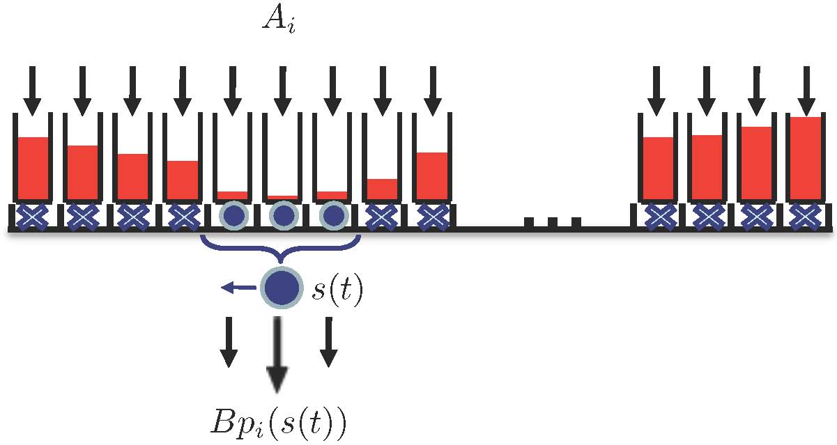
Viewing persistent monitoring as a polling system, each point αisubscript𝛼𝑖\alpha_{i} (equivalently, i𝑖ith interval in [0,L]0𝐿[0,L]) is associated with a “virtual queue” where uncertainty accumulates with inflow rate Aisubscript𝐴𝑖A_{i}. The service rate of this queue is time-varying and given by BPi(𝐬(t))𝐵subscript𝑃𝑖𝐬𝑡BP_{i}\left(\mathbf{s}(t)\right), controllable through the agent position at time t𝑡t. Figure 1 illustrates this polling system when N=1𝑁1N=1. This interpretation is convenient for characterizing the stability of such a system over a mission time T𝑇T: For each queue, we may require that 0TAi<0TBpi(s(t))𝑑tsuperscriptsubscript0𝑇subscript𝐴𝑖superscriptsubscript0𝑇𝐵subscript𝑝𝑖𝑠𝑡differential-d𝑡\int_{0}^{T}A_{i}<\int_{0}^{T}Bp_{i}(s(t))dt. Alternatively, we may require that each queue becomes empty at least once over [0,T]0𝑇[0,T]. We may also impose conditions such as Ri(T)Rmaxsubscript𝑅𝑖𝑇subscript𝑅R_{i}(T)\leq R_{\max} for each queue as additional constraints for our problem so as to provide bounded uncertainty guarantees, although we will not do so in this paper. Note that this analogy readily extends to 2 or 3-dimensional settings.
Refer to caption
Figure 1: A queueing system analog of the persistent monitoring problem.

The goal of the optimal persistent monitoring problem we consider is to control the movement of the N𝑁N agents through un(t)subscript𝑢𝑛𝑡u_{n}\left(t\right) in (1) so that the cumulative uncertainty over all sensing points {αi},subscript𝛼𝑖\{\alpha_{i}\}, i=1,,M𝑖1𝑀i=1,\ldots,M is minimized over a fixed time horizon T𝑇T. Thus, setting 𝐮(t)=[u1(t),,uN(t)]𝐮𝑡subscript𝑢1𝑡subscript𝑢𝑁𝑡\mathbf{u}\left(t\right)=\left[u_{1}\left(t\right),\ldots,u_{N}\left(t\right)\right] we aim to solve the following optimal control problem P1:

min𝐮(t) J=1T0Ti=1MRi(t)dtsubscript𝐮𝑡 𝐽1𝑇superscriptsubscript0𝑇superscriptsubscript𝑖1𝑀subscript𝑅𝑖𝑡𝑑𝑡\min_{\mathbf{u}\left(t\right)}\text{ \ }J=\frac{1}{T}\int_{0}^{T}\sum_{i=1}^{M}R_{i}(t)dt (7)

subject to the agent dynamics (1), uncertainty dynamics (6), control constraint |un(t)|1subscript𝑢𝑛𝑡1|u_{n}(t)|\leq 1, t[0,T]𝑡0𝑇t\in[0,T], and state constraints (2), t[0,T]𝑡0𝑇t\in[0,T]. Note that we require arn𝑎subscript𝑟𝑛a\leq r_{n} and bLrm𝑏𝐿subscript𝑟𝑚b\geq L-r_{m}, for at least some n,m=1,,Nformulae-sequence𝑛𝑚1𝑁n,m=1,\ldots,N; this is to ensure that there are no points in [0,L]0𝐿[0,L] which can never be sensed, i.e., any i𝑖i such that αi<arnsubscript𝛼𝑖𝑎subscript𝑟𝑛\alpha_{i}<a-r_{n} or αi>b+rnsubscript𝛼𝑖𝑏subscript𝑟𝑛\alpha_{i}>b+r_{n} would always lie outside any agent’s sensing range. We will omit the additional constraint (3) from our initial analysis, but we will show that, when it is included, the optimal solution never allows it to be active.

3 Optimal Control Solution

3.1 Hamiltonian analysis

We first characterize the optimal control solution of problem P1 and show that it can be reduced to a parametric optimization problem. This allows us to utilize an Infinitesimal Perturbation Analysis (IPA) gradient estimation approach [15] to find a complete optimal solution through a gradient-based algorithm. We define the state vector 𝐱(t)=[s1(t),,sN(t),R1(t),,RM(t)]𝚃𝐱𝑡superscriptsubscript𝑠1𝑡subscript𝑠𝑁𝑡subscript𝑅1𝑡subscript𝑅𝑀𝑡𝚃\mathbf{x}\left(t\right)=[s_{1}\left(t\right),\ldots,s_{N}\left(t\right),R_{1}\left(t\right),\ldots,R_{M}\left(t\right)]^{\mathtt{T}} and the associated costate vector λ(t)=𝜆𝑡absent\mathbf{\lambda}\left(t\right)= [λs1(t),,λsN(t),λ1(t),,λM(t)]𝚃superscriptsubscript𝜆subscript𝑠1𝑡subscript𝜆subscript𝑠𝑁𝑡subscript𝜆1𝑡subscript𝜆𝑀𝑡𝚃[\lambda_{s_{1}}\left(t\right),\ldots,\lambda_{s_{N}}\left(t\right),\lambda_{1}\left(t\right),\ldots,\lambda_{M}\left(t\right)]^{\mathtt{T}}. In view of the discontinuity in the dynamics of Ri(t)subscript𝑅𝑖𝑡R_{i}(t) in (6), the optimal state trajectory may contain a boundary arc when Ri(t)=0subscript𝑅𝑖𝑡0R_{i}(t)=0 for any i𝑖i; otherwise, the state evolves in an interior arc. We first analyze the system operating in such an interior arc and omit the constraint (2) as well. Using (1) and (6), the Hamiltonian is

H(𝐱,λ,𝐮)=i=1MRi(t)+n=1Nλsn(t)un(t)+i=1Mλi(t)R˙i(t)𝐻𝐱𝜆𝐮superscriptsubscript𝑖1𝑀subscript𝑅𝑖𝑡superscriptsubscript𝑛1𝑁subscript𝜆subscript𝑠𝑛𝑡subscript𝑢𝑛𝑡superscriptsubscript𝑖1𝑀subscript𝜆𝑖𝑡subscript˙𝑅𝑖𝑡H\left(\mathbf{x},\mathbf{\lambda},\mathbf{u}\right)=\sum_{i=1}^{M}R_{i}\left(t\right)+\sum_{n=1}^{N}\lambda_{s_{n}}\left(t\right)u_{n}\left(t\right)+\sum_{i=1}^{M}\lambda_{i}\left(t\right)\dot{R}_{i}(t) (8)

and the costate equations λ˙=Hx˙𝜆𝐻𝑥\mathbf{\dot{\lambda}}=-\frac{\partial H}{\partial x} are

λ˙i(t)subscript˙𝜆𝑖𝑡\displaystyle\dot{\lambda}_{i}\left(t\right) =HRi(t)=1i=1,,Mformulae-sequenceabsent𝐻subscript𝑅𝑖𝑡1𝑖1𝑀\displaystyle=-\frac{\partial H}{\partial R_{i}\left(t\right)}=-1\text{, \ \ }i=1,\ldots,M (9)
λ˙sn(t)subscript˙𝜆subscript𝑠𝑛𝑡\displaystyle\dot{\lambda}_{s_{n}}\left(t\right) =Hsn(t)=Brniϝn(t)λi(t)dn[1pd,i(sd(t))]+Brniϝn+(t)λi(t)dn[1pd,i(sd(t))]absent𝐻subscript𝑠𝑛𝑡𝐵subscript𝑟𝑛subscript𝑖superscriptsubscriptitalic-ϝ𝑛𝑡subscript𝜆𝑖𝑡subscriptproduct𝑑𝑛delimited-[]1subscript𝑝𝑑𝑖subscript𝑠𝑑𝑡𝐵subscript𝑟𝑛subscript𝑖superscriptsubscriptitalic-ϝ𝑛𝑡subscript𝜆𝑖𝑡subscriptproduct𝑑𝑛delimited-[]1subscript𝑝𝑑𝑖subscript𝑠𝑑𝑡\displaystyle=-\frac{\partial H}{\partial s_{n}\left(t\right)}=-\frac{B}{r_{n}}\sum_{i\in\digamma_{n}^{-}\left(t\right)}\lambda_{i}\left(t\right){\displaystyle\prod\limits_{d\neq n}}\left[1-p_{d,i}(s_{d}\left(t\right))\right]+\frac{B}{r_{n}}\sum_{i\in\digamma_{n}^{+}\left(t\right)}\lambda_{i}\left(t\right){\displaystyle\prod\limits_{d\neq n}}\left[1-p_{d,i}(s_{d}\left(t\right))\right] (10)

where we have used (4), and the sets ϝn(t)superscriptsubscriptitalic-ϝ𝑛𝑡\digamma_{n}^{-}(t) and ϝn+(t)superscriptsubscriptitalic-ϝ𝑛𝑡\digamma_{n}^{+}(t) are defined as

ϝn(t)superscriptsubscriptitalic-ϝ𝑛𝑡\displaystyle\digamma_{n}^{-}(t) ={i:sn(t)rnαisn(t)}absentconditional-set𝑖subscript𝑠𝑛𝑡subscript𝑟𝑛subscript𝛼𝑖subscript𝑠𝑛𝑡\displaystyle=\{i:s_{n}\left(t\right)-r_{n}\leq\alpha_{i}\leq s_{n}\left(t\right)\}\text{ \ } (11)
ϝn+(t)superscriptsubscriptitalic-ϝ𝑛𝑡\displaystyle\digamma_{n}^{+}(t) ={i:sn(t)<αisn(t)+rn}absentconditional-set𝑖subscript𝑠𝑛𝑡subscript𝛼𝑖subscript𝑠𝑛𝑡subscript𝑟𝑛\displaystyle=\{i:s_{n}\left(t\right)<\alpha_{i}\leq s_{n}\left(t\right)+r_{n}\}

for n=1,,N𝑛1𝑁n=1,\ldots,N. Note that ϝn(t)superscriptsubscriptitalic-ϝ𝑛𝑡\digamma_{n}^{-}(t), ϝn+(t)superscriptsubscriptitalic-ϝ𝑛𝑡\digamma_{n}^{+}(t) identify all points αisubscript𝛼𝑖\alpha_{i} to the left and right of sn(t)subscript𝑠𝑛𝑡s_{n}\left(t\right) respectively that are within agent n𝑛n’s sensing range. Since we impose no terminal state constraints, the boundary conditions are λi(T)=0subscript𝜆𝑖𝑇0\lambda_{i}\left(T\right)=0,  i=1,,M𝑖1𝑀i=1,\ldots,M and λsn(T)=0subscript𝜆subscript𝑠𝑛𝑇0\lambda_{s_{n}}\left(T\right)=0,  n=1,,N.𝑛1𝑁n=1,...,N. Applying the Pontryagin minimum principle to (8) with 𝐮(t)superscript𝐮𝑡\mathbf{u}^{\star}(t), t[0,T)𝑡0𝑇t\in[0,T), denoting an optimal control, we have

H(𝐱,λ,𝐮)=minun[1,1], n=1,,NH(𝐱,λ,𝐮)𝐻superscript𝐱superscript𝜆superscript𝐮subscriptformulae-sequencesubscript𝑢𝑛11 𝑛1𝑁𝐻𝐱𝜆𝐮H\left(\mathbf{x}^{\star},\mathbf{\lambda}^{\star},\mathbf{u}^{\star}\right)=\min_{u_{n}\in[-1,1],\text{ }n=1,\ldots,N}H\left(\mathbf{x},\mathbf{\lambda},\mathbf{u}\right)

and it is immediately obvious that it is necessary for an optimal control to satisfy:

un(t)={1 if λsn(t)<01 if λsn(t)>0superscriptsubscript𝑢𝑛𝑡cases1 if subscript𝜆subscript𝑠𝑛𝑡01 if subscript𝜆subscript𝑠𝑛𝑡0u_{n}^{\star}(t)=\left\{\begin{array}[c]{ll}1&\text{ if }\lambda_{s_{n}}\left(t\right)<0\\ -1&\text{ if }\lambda_{s_{n}}\left(t\right)>0\end{array}\right. (12)

This condition excludes the possibility that λsn(t)=0subscript𝜆subscript𝑠𝑛𝑡0\lambda_{s_{n}}\left(t\right)=0 over some finite singular intervals [17]. We will show that if sn(t)=a>0subscript𝑠𝑛𝑡𝑎0s_{n}\left(t\right)=a>0 or sn(t)=b<L,subscript𝑠𝑛𝑡𝑏𝐿s_{n}\left(t\right)=b<L, then λsn(t)=0subscript𝜆subscript𝑠𝑛𝑡0\lambda_{s_{n}}\left(t\right)=0 for some n{1,,N}𝑛1𝑁n\in\left\{1,\ldots,N\right\} may in fact exist for some finite arc; otherwise λsn(t)=0subscript𝜆subscript𝑠𝑛𝑡0\lambda_{s_{n}}\left(t\right)=0 can arise only when un(t)=0subscript𝑢𝑛𝑡0u_{n}\left(t\right)=0.

The implication of (9) with λi(T)=0subscript𝜆𝑖𝑇0\lambda_{i}\left(T\right)=0 is that λi(t)=Ttsubscript𝜆𝑖𝑡𝑇𝑡\lambda_{i}\left(t\right)=T-t for all t[0,T]𝑡0𝑇t\in[0,T] and all i=1,,M𝑖1𝑀i=1,\ldots,M and that λi(t)subscript𝜆𝑖𝑡\lambda_{i}\left(t\right) is monotonically decreasing starting with λi(0)=Tsubscript𝜆𝑖0𝑇\lambda_{i}\left(0\right)=T. However, this is only true if the entire optimal trajectory is an interior arc, i.e., all Ri(t)0subscript𝑅𝑖𝑡0R_{i}(t)\geq 0 constraints for all i=1,,M𝑖1𝑀i=1,\ldots,M remain inactive. On the other hand, looking at (10), observe that when the two end points, 00 and L𝐿L, are not within the range of an agent, we have |Fn(t)|=|Fn+(t)|superscriptsubscript𝐹𝑛𝑡superscriptsubscript𝐹𝑛𝑡\left|F_{n}^{-}(t)\right|=\left|F_{n}^{+}(t)\right|, since the number of indices i𝑖i satisfying sn(t)rnαisn(t)subscript𝑠𝑛𝑡subscript𝑟𝑛subscript𝛼𝑖subscript𝑠𝑛𝑡s_{n}\left(t\right)-r_{n}\leq\alpha_{i}\leq s_{n}\left(t\right) is the same as that satisfying sn(t)<αisn(t)+rnsubscript𝑠𝑛𝑡subscript𝛼𝑖subscript𝑠𝑛𝑡subscript𝑟𝑛s_{n}\left(t\right)<\alpha_{i}\leq s_{n}\left(t\right)+r_{n}. Consequently, for the one-agent case N=1𝑁1N=1, (10) becomes

λ˙s1(t)=Br1iF1(t)λi(t)+Br1iF1+(t)λi(t)subscript˙𝜆subscript𝑠1𝑡𝐵subscript𝑟1subscript𝑖superscriptsubscript𝐹1𝑡subscript𝜆𝑖𝑡𝐵subscript𝑟1subscript𝑖superscriptsubscript𝐹1𝑡subscript𝜆𝑖𝑡\dot{\lambda}_{s_{1}}\left(t\right)=-\frac{B}{r_{1}}\sum_{i\in F_{1}^{-}(t)}\lambda_{i}(t)+\frac{B}{r_{1}}\sum_{i\in F_{1}^{+}(t)}\lambda_{i}(t) (13)

and λ˙s1(t)=0subscript˙𝜆subscript𝑠1𝑡0\dot{\lambda}_{s_{1}}\left(t\right)=0 since the two terms in (13) will cancel out, i.e., λs1(t)subscript𝜆subscript𝑠1𝑡\lambda_{s_{1}}\left(t\right) remains constant as long as this condition is satisfied and, in addition, none of the state constraints Ri(t)0subscript𝑅𝑖𝑡0R_{i}(t)\geq 0, i=1,,M𝑖1𝑀i=1,\ldots,M, is active. Thus, for the one agent case, as long as the optimal trajectory is an interior arc and λs1(t)<0subscript𝜆subscript𝑠1𝑡0\lambda_{s_{1}}\left(t\right)<0, the agent moves at maximal speed u1(t)=1superscriptsubscript𝑢1𝑡1u_{1}^{\star}\left(t\right)=1 in the positive direction towards the point s1=bsubscript𝑠1𝑏s_{1}=b. If λs1(t)subscript𝜆subscript𝑠1𝑡\lambda_{s_{1}}\left(t\right) switches sign before any of the state constraints Ri(t)0subscript𝑅𝑖𝑡0R_{i}(t)\geq 0, i=1,,M𝑖1𝑀i=1,\ldots,M, becomes active or the agent reaches the end point s1=bsubscript𝑠1𝑏s_{1}=b, then u1(t)=1superscriptsubscript𝑢1𝑡1u_{1}^{\star}\left(t\right)=-1 and the agent reverses its direction or, possibly, comes to rest.

In what follows, we examine the effect of the state constraints which significantly complicates the analysis, leading to a challenging two-point-boundary-value problem. However, we will establish the fact that the complete solution boils down to determining a set of switching locations over [a,b]𝑎𝑏[a,b] and waiting times at these switching points, with the end points, 00 and L𝐿L, being always infeasible on an optimal trajectory. This is a much simpler problem that we are subsequently able to solve.

We begin by recalling that the dynamics in (6) indicate a discontinuity arising when the condition Ri(t)=0subscript𝑅𝑖𝑡0R_{i}(t)=0 is satisfied while R˙i(t)=AiBPi(𝐬(t))<0subscript˙𝑅𝑖𝑡subscript𝐴𝑖𝐵subscript𝑃𝑖𝐬𝑡0\dot{R}_{i}(t)=A_{i}-BP_{i}\left(\mathbf{s}(t)\right)<0 for some i=1,,M𝑖1𝑀i=1,\ldots,M. Thus, Ri=0subscript𝑅𝑖0R_{i}=0 defines an interior boundary condition which is not an explicit function of time. Following standard optimal control analysis [17], if this condition is satisfied at time t𝑡t for some j{1,,M}𝑗1𝑀j\in\{1,\ldots,M\},

H(𝐱(t),λ(t),𝐮(t))=H(𝐱(t+),λ(t+),𝐮(t+))𝐻𝐱superscript𝑡𝜆superscript𝑡𝐮superscript𝑡𝐻𝐱superscript𝑡𝜆superscript𝑡𝐮superscript𝑡H\left(\mathbf{x}(t^{-}),\mathbf{\lambda}(t^{-}),\mathbf{u}(t^{-})\right)=H\left(\mathbf{x}(t^{+}),\mathbf{\lambda}(t^{+}),\mathbf{u}(t^{+})\right) (14)

where we note that one can choose to set the Hamiltonian to be continuous at the entry point of a boundary arc or at the exit point. Using (8) and (6), (14) implies:

n=1Nλsn(t)un(t)+λj(t)[Aj(t)BPj(𝐬(t))]=n=1Nλsn(t+)un(t+)superscriptsubscript𝑛1𝑁superscriptsubscript𝜆subscript𝑠𝑛superscript𝑡superscriptsubscript𝑢𝑛superscript𝑡superscriptsubscript𝜆𝑗superscript𝑡delimited-[]subscript𝐴𝑗𝑡𝐵subscript𝑃𝑗𝐬𝑡superscriptsubscript𝑛1𝑁superscriptsubscript𝜆subscript𝑠𝑛superscript𝑡superscriptsubscript𝑢𝑛superscript𝑡\sum_{n=1}^{N}\lambda_{s_{n}}^{\ast}\left(t^{-}\right)u_{n}^{\ast}\left(t^{-}\right)+\lambda_{j}^{\star}\left(t^{-}\right)[A_{j}\left(t\right)-BP_{j}(\mathbf{s}(t))]=\sum_{n=1}^{N}\lambda_{s_{n}}^{\ast}\left(t^{+}\right)u_{n}^{\ast}\left(t^{+}\right) (15)

In addition, λsn(t)=λsn(t+)superscriptsubscript𝜆subscript𝑠𝑛superscript𝑡superscriptsubscript𝜆subscript𝑠𝑛superscript𝑡\lambda_{s_{n}}^{\star}\left(t^{-}\right)=\lambda_{s_{n}}^{\star}\left(t^{+}\right) for all n=𝑛absentn= 1,,N1𝑁1,\ldots,N and λi(t)=λi(t+)superscriptsubscript𝜆𝑖superscript𝑡superscriptsubscript𝜆𝑖superscript𝑡\lambda_{i}^{\star}\left(t^{-}\right)=\lambda_{i}^{\star}\left(t^{+}\right) for all ij𝑖𝑗i\neq j, but λj(t)superscriptsubscript𝜆𝑗𝑡\lambda_{j}^{\star}\left(t\right) may experience a discontinuity so that:

λj(t)=λj(t+)πjsuperscriptsubscript𝜆𝑗superscript𝑡superscriptsubscript𝜆𝑗superscript𝑡subscript𝜋𝑗\lambda_{j}^{\star}\left(t^{-}\right)=\lambda_{j}^{\star}\left(t^{+}\right)-\pi_{j} (16)

where πj0subscript𝜋𝑗0\pi_{j}\geq 0 is a multiplier associated with the constraint Rj(t)0subscript𝑅𝑗𝑡0-R_{j}(t)\leq 0. Recalling (12), since λsn(t)superscriptsubscript𝜆subscript𝑠𝑛𝑡\lambda_{s_{n}}^{\star}\left(t\right) remains unaffected, so does the optimal control, i.e., un(t)=un(t+)superscriptsubscript𝑢𝑛superscript𝑡superscriptsubscript𝑢𝑛superscript𝑡u_{n}^{\star}(t^{-})=u_{n}^{\star}(t^{+}). Moreover, since this is an entry point of a boundary arc, it follows from (6) that AjBPj(𝐬(t))<0subscript𝐴𝑗𝐵subscript𝑃𝑗𝐬𝑡0A_{j}-BP_{j}\left(\mathbf{s}(t)\right)<0. Therefore, (15) and (16) imply that

λj(t)=0, λj(t+)=πj0.formulae-sequencesuperscriptsubscript𝜆𝑗superscript𝑡0 superscriptsubscript𝜆𝑗superscript𝑡subscript𝜋𝑗0\lambda_{j}^{\star}\left(t^{-}\right)=0,\text{ \ }\lambda_{j}^{\star}\left(t^{+}\right)=\pi_{j}\geq 0.

Thus, λi(t)subscript𝜆𝑖𝑡\lambda_{i}\left(t\right) always decreases with constant rate 11-1 until Ri(t)=0subscript𝑅𝑖𝑡0R_{i}\left(t\right)=0 is active, at which point λi(t)subscript𝜆𝑖𝑡\lambda_{i}\left(t\right) jumps to a non-negative value πisubscript𝜋𝑖\pi_{i} and decreases with rate 11-1 again. The value of πisubscript𝜋𝑖\pi_{i} is determined by how long it takes for the agents to reduce Ri(t)subscript𝑅𝑖𝑡R_{i}\left(t\right) to 00 once again. Obviously,

λi(t)0, i=1,,Mt[0,T]formulae-sequencesubscript𝜆𝑖𝑡0formulae-sequence 𝑖1𝑀𝑡0𝑇\lambda_{i}\left(t\right)\geq 0,\text{ }i=1,\ldots,M\text{, }t\in\left[0,T\right] (17)

with equality holding only if t=T,𝑡𝑇t=T, or t=𝑡absentt= t0superscriptsubscript𝑡0t_{0}^{-} with Ri(t0)=0subscript𝑅𝑖subscript𝑡00R_{i}\left(t_{0}\right)=0, Ri(t)>0subscript𝑅𝑖superscript𝑡0R_{i}\left(t^{\prime}\right)>0, where t[t0δ,t0)superscript𝑡subscript𝑡0𝛿subscript𝑡0t^{\prime}\in[t_{0}-\delta,t_{0}), δ>0.𝛿0\delta>0. The actual evaluation of the costate vector over the interval [0,T]0𝑇[0,T] requires solving (10), which in turn involves the determination of all points where the state variables Ri(t)subscript𝑅𝑖𝑡R_{i}(t) reach their minimum feasible values Ri(t)=0subscript𝑅𝑖𝑡0R_{i}(t)=0, i=1,,M𝑖1𝑀i=1,\ldots,M. This generally involves the solution of a two-point-boundary-value problem. However, our analysis thus far has already established the structure of the optimal control (12) which we have seen to remain unaffected by the presence of boundary arcs when Ri(t)=0subscript𝑅𝑖𝑡0R_{i}(t)=0 for one or more i=1,,M𝑖1𝑀i=1,\ldots,M. We will next prove some additional structural properties of an optimal trajectory, based on which we show that it is fully characterized by a set of non-negative scalar parameters. Determining the values of these parameters is a much simpler problem that does not require the solution of a two-point-boundary-value problem.

Let us turn our attention to the constraints sn(t)asubscript𝑠𝑛𝑡𝑎s_{n}(t)\geq a and sn(t)bsubscript𝑠𝑛𝑡𝑏s_{n}(t)\leq b and consider first the case where a=0𝑎0a=0, b=L𝑏𝐿b=L, i.e., the agents can move over the entire [0,L]0𝐿[0,L]. We shall make use of the following technical condition:

Assumption 1: For any n=1,,N𝑛1𝑁n=1,\ldots,N, i=1,,M𝑖1𝑀i=1,\ldots,M, t(0,T)𝑡0𝑇t\in(0,T), and any ϵ>0italic-ϵ0\epsilon>0, if sn(t)=0subscript𝑠𝑛𝑡0s_{n}(t)=0, sn(tϵ)>0subscript𝑠𝑛𝑡italic-ϵ0s_{n}(t-\epsilon)>0, then either Ri(τ)>0subscript𝑅𝑖𝜏0R_{i}(\tau)>0 for all τ[tϵ,t]𝜏𝑡italic-ϵ𝑡\tau\in[t-\epsilon,t] or Ri(τ)=0subscript𝑅𝑖𝜏0R_{i}(\tau)=0 for all τ[tϵ,t]𝜏𝑡italic-ϵ𝑡\tau\in[t-\epsilon,t]; if sn(t)=L,sn(tϵ)<Lformulae-sequencesubscript𝑠𝑛𝑡𝐿subscript𝑠𝑛𝑡italic-ϵ𝐿s_{n}(t)=L,s_{n}(t-\epsilon)<L,then either Ri(τ)>0subscript𝑅𝑖𝜏0R_{i}(\tau)>0 for all τ[tϵ,t]𝜏𝑡italic-ϵ𝑡\tau\in[t-\epsilon,t] or Ri(τ)=0subscript𝑅𝑖𝜏0R_{i}(\tau)=0 for all τ[tϵ,t]𝜏𝑡italic-ϵ𝑡\tau\in[t-\epsilon,t].

This condition excludes the case where an agent reaches an endpoint of the mission space at the exact same time that any one of the uncertainty functions reaches its minimal value of zero. Then, the following proposition asserts that neither of the constraints sn(t)0subscript𝑠𝑛𝑡0s_{n}(t)\geq 0 and sn(t)Lsubscript𝑠𝑛𝑡𝐿s_{n}(t)\leq L can become active on an optimal trajectory.

Proposition 3.1

Under Assumption 1, if a=0𝑎0a=0, b=L𝑏𝐿b=L, then on an optimal trajectory: sn(t)0superscriptsubscript𝑠𝑛𝑡0s_{n}^{\star}\left(t\right)\neq 0 and sn(t)Lsuperscriptsubscript𝑠𝑛𝑡𝐿s_{n}^{\star}\left(t\right)\neq L for all t(0,T)𝑡0𝑇t\in(0,T), n{1,,N}.𝑛1𝑁n\in\left\{1,\ldots,N\right\}.

Proof. Suppose at t=t0<T𝑡subscript𝑡0𝑇t=t_{0}<T an agent reaches the left endpoint, i.e., sn(t0)=0superscriptsubscript𝑠𝑛subscript𝑡00s_{n}^{\ast}\left(t_{0}\right)=0, sn(t0)>0superscriptsubscript𝑠𝑛superscriptsubscript𝑡00s_{n}^{\ast}\left(t_{0}^{-}\right)>0. We will then establish a contradiction. Thus, assuming sn(t0)=0superscriptsubscript𝑠𝑛subscript𝑡00s_{n}^{\ast}\left(t_{0}\right)=0, we first show that λsn(t0)=0superscriptsubscript𝜆subscript𝑠𝑛superscriptsubscript𝑡00\lambda_{s_{n}}^{\ast}\left(t_{0}^{-}\right)=0 by a contradiction argument. Assume that λsn(t0)0superscriptsubscript𝜆subscript𝑠𝑛superscriptsubscript𝑡00\lambda_{s_{n}}^{\ast}\left(t_{0}^{-}\right)\neq 0, in which case, since the agent is moving toward sn=0subscript𝑠𝑛0s_{n}=0, we have un(t0)=1superscriptsubscript𝑢𝑛superscriptsubscript𝑡01u_{n}^{\ast}\left(t_{0}^{-}\right)=-1 and λsn(t0)>0superscriptsubscript𝜆subscript𝑠𝑛superscriptsubscript𝑡00\lambda_{s_{n}}^{\ast}\left(t_{0}^{-}\right)>0 from (12). Then, λsn(t)superscriptsubscript𝜆subscript𝑠𝑛𝑡\lambda_{s_{n}}^{\ast}\left(t\right) may experience a discontinuity so that

λsn(t0)=λsn(t0+)πnsuperscriptsubscript𝜆subscript𝑠𝑛superscriptsubscript𝑡0superscriptsubscript𝜆subscript𝑠𝑛superscriptsubscript𝑡0subscript𝜋𝑛\lambda_{s_{n}}^{\ast}\left(t_{0}^{-}\right)=\lambda_{s_{n}}^{\ast}\left(t_{0}^{+}\right)-\pi_{n} (18)

where πn0subscript𝜋𝑛0\pi_{n}\geqslant 0 is a scalar constant. It follows that λsn(t0+)=λsn(t0)+πn>0superscriptsubscript𝜆subscript𝑠𝑛superscriptsubscript𝑡0superscriptsubscript𝜆subscript𝑠𝑛superscriptsubscript𝑡0subscript𝜋𝑛0\lambda_{s_{n}}^{\ast}\left(t_{0}^{+}\right)=\lambda_{s_{n}}^{\ast}\left(t_{0}^{-}\right)+\pi_{n}>0. Since the constraint sn(t)=0subscript𝑠𝑛𝑡0s_{n}\left(t\right)=0 is not an explicit function of time, we have

λsn(t0)un(t0)=λsn(t0+)un(t0+)superscriptsubscript𝜆subscript𝑠𝑛superscriptsubscript𝑡0superscriptsubscript𝑢𝑛superscriptsubscript𝑡0superscriptsubscript𝜆subscript𝑠𝑛superscriptsubscript𝑡0superscriptsubscript𝑢𝑛superscriptsubscript𝑡0\lambda_{s_{n}}^{\ast}\left(t_{0}^{-}\right)u_{n}^{\ast}\left(t_{0}^{-}\right)=\lambda_{s_{n}}^{\ast}\left(t_{0}^{+}\right)u_{n}^{\ast}\left(t_{0}^{+}\right) (19)

On the other hand, un(t0+)0superscriptsubscript𝑢𝑛superscriptsubscript𝑡00u_{n}^{\ast}\left(t_{0}^{+}\right)\geqslant 0, since agent n𝑛n must either come to rest or reverse its motion at sn=0subscript𝑠𝑛0s_{n}=0, hence λsn(t0+)un(t0+)0superscriptsubscript𝜆subscript𝑠𝑛superscriptsubscript𝑡0superscriptsubscript𝑢𝑛superscriptsubscript𝑡00\lambda_{s_{n}}^{\ast}\left(t_{0}^{+}\right)u_{n}^{\ast}\left(t_{0}^{+}\right)\geqslant 0. This violates (19), since λsn(t0)un(t0)<0.superscriptsubscript𝜆subscript𝑠𝑛superscriptsubscript𝑡0superscriptsubscript𝑢𝑛superscriptsubscript𝑡00\lambda_{s_{n}}^{\ast}\left(t_{0}^{-}\right)u_{n}^{\ast}\left(t_{0}^{-}\right)<0. This contradiction implies that λsn(t0)=0superscriptsubscript𝜆subscript𝑠𝑛superscriptsubscript𝑡00\lambda_{s_{n}}^{\ast}\left(t_{0}^{-}\right)=0. Next, consider (10) and observe that in (11) we have Fn(t0)=superscriptsubscript𝐹𝑛subscript𝑡0F_{n}^{-}\left(t_{0}\right)=\varnothing, since αi>sn(t0)=0subscript𝛼𝑖superscriptsubscript𝑠𝑛subscript𝑡00\alpha_{i}>s_{n}^{\ast}\left(t_{0}\right)=0 for all i=1,,M𝑖1𝑀i=1,\ldots,M. Therefore, recalling (17), it follows from (10) that

λ˙sn(t0)=Brniϝn+(t0)λi(t0)dn[1pd,i(sd(t0))]0subscript˙𝜆subscript𝑠𝑛superscriptsubscript𝑡0𝐵subscript𝑟𝑛subscript𝑖superscriptsubscriptitalic-ϝ𝑛superscriptsubscript𝑡0subscript𝜆𝑖superscriptsubscript𝑡0subscriptproduct𝑑𝑛delimited-[]1subscript𝑝𝑑𝑖subscript𝑠𝑑superscriptsubscript𝑡00\dot{\lambda}_{s_{n}}\left(t_{0}^{-}\right)=\frac{B}{r_{n}}\sum_{i\in\digamma_{n}^{+}\left(t_{0}^{-}\right)}\lambda_{i}\left(t_{0}^{-}\right){\displaystyle\prod\limits_{d\neq n}}\left[1-p_{d,i}(s_{d}\left(t_{0}^{-}\right))\right]\geq 0

Under Assumption 1, there exists δ1>0subscript𝛿10\delta_{1}>0 such that during the interval (t0δ1,t0)subscript𝑡0subscript𝛿1subscript𝑡0(t_{0}-\delta_{1},t_{0}) no Ri(t)0subscript𝑅𝑖𝑡0R_{i}\left(t\right)\geq 0 becomes active, hence no λi(t)subscript𝜆𝑖𝑡\lambda_{i}(t) encounters a jump for i=1,,M𝑖1𝑀i=1,\ldots,M. It follows that λi(t)>0superscriptsubscript𝜆𝑖𝑡0\lambda_{i}^{\ast}(t)>0 for iFn+(t)𝑖superscriptsubscript𝐹𝑛𝑡i\in F_{n}^{+}(t) and λ˙sn(t)superscriptsubscript˙𝜆subscript𝑠𝑛𝑡\dot{\lambda}_{s_{n}}^{\ast}\left(t\right) is continuous with λ˙sn(t)>0superscriptsubscript˙𝜆subscript𝑠𝑛𝑡0\dot{\lambda}_{s_{n}}^{\ast}\left(t\right)>0 for t(t0δ1,t0)𝑡subscript𝑡0subscript𝛿1subscript𝑡0t\in(t_{0}-\delta_{1},t_{0}). Again, since sn(t0)=0,superscriptsubscript𝑠𝑛subscript𝑡00s_{n}^{\ast}\left(t_{0}\right)=0, there exists some δ2δ1subscript𝛿2subscript𝛿1\delta_{2}\leq\delta_{1} such that for t(t0δ2,t0)𝑡subscript𝑡0subscript𝛿2subscript𝑡0t\in\left(t_{0}-\delta_{2},t_{0}\right), we have un(t)<0superscriptsubscript𝑢𝑛𝑡0u_{n}^{\ast}\left(t\right)<0 and λsn(t)0superscriptsubscript𝜆subscript𝑠𝑛𝑡0\lambda_{s_{n}}^{\ast}\left(t\right)\geq 0. Thus, for t(t0δ2,t0)𝑡subscript𝑡0subscript𝛿2subscript𝑡0t\in\left(t_{0}-\delta_{2},t_{0}\right), we have λsn(t)0superscriptsubscript𝜆subscript𝑠𝑛𝑡0\lambda_{s_{n}}^{\ast}\left(t\right)\geq 0 and λ˙sn(t)superscriptsubscript˙𝜆subscript𝑠𝑛𝑡\dot{\lambda}_{s_{n}}^{\ast}\left(t\right) >0absent0>0. This contradicts the fact we already established that λsn(t0)=0superscriptsubscript𝜆subscript𝑠𝑛superscriptsubscript𝑡00\lambda_{s_{n}}^{\ast}\left(t_{0}^{-}\right)=0 and we conclude that sn(t)0superscriptsubscript𝑠𝑛𝑡0s_{n}^{\star}\left(t\right)\neq 0 for all t[0,T]𝑡0𝑇t\in\left[0,T\right], n=1,,N𝑛1𝑁n=1,\ldots,N. Using a similar line of argument, we can also show that sn(t)Lsuperscriptsubscript𝑠𝑛𝑡𝐿s_{n}^{\ast}\left(t\right)\neq L. \blacksquare

Proposition 3.2

If a>0𝑎0a>0 and (or) b<L𝑏𝐿b<L, then on an optimal trajectory there exist finite length intervals [t0,t1]subscript𝑡0subscript𝑡1[t_{0},t_{1}] such that sn(t)=asubscript𝑠𝑛𝑡𝑎s_{n}\left(t\right)=a and (or) sn(t)=bsubscript𝑠𝑛𝑡𝑏s_{n}\left(t\right)=b, for some n{1,,N}𝑛1𝑁n\in\left\{1,\ldots,N\right\}, t[t0,t1]𝑡subscript𝑡0subscript𝑡1t\in[t_{0},t_{1}], 0t0<0subscript𝑡0absent0\leq t_{0}< t1Tsubscript𝑡1𝑇t_{1}\leq T.

Proof. Proceeding as in the proof of Proposition 3.1, when sn(t0)=asuperscriptsubscript𝑠𝑛subscript𝑡0𝑎s_{n}^{\ast}\left(t_{0}\right)=a we can establish (19) and the fact that λsn(t0)=0superscriptsubscript𝜆subscript𝑠𝑛superscriptsubscript𝑡00\lambda_{s_{n}}^{\ast}\left(t_{0}^{-}\right)=0. On the other hand, un(t0+)0superscriptsubscript𝑢𝑛superscriptsubscript𝑡00u_{n}^{\ast}\left(t_{0}^{+}\right)\geqslant 0, since the agent must either come to rest or reverse its motion at sn(t0)=asubscript𝑠𝑛subscript𝑡0𝑎s_{n}\left(t_{0}\right)=a. In other words, when sn(t0)=asubscript𝑠𝑛subscript𝑡0𝑎s_{n}\left(t_{0}\right)=a on an optimal trajectory, (19) is satisfied either with the agent reversing its direction immediately (in which case t1=t0subscript𝑡1subscript𝑡0t_{1}=t_{0} and λsn(t0+)=0superscriptsubscript𝜆subscript𝑠𝑛superscriptsubscript𝑡00\lambda_{s_{n}}^{\ast}\left(t_{0}^{+}\right)=0) or staying on the boundary arc for a finite time interval (in which case t1>t0subscript𝑡1subscript𝑡0t_{1}>t_{0} and un(t)=0superscriptsubscript𝑢𝑛𝑡0u_{n}^{\ast}\left(t\right)=0 for t[t0,t1]𝑡subscript𝑡0subscript𝑡1t\in[t_{0},t_{1}]). The exact same argument can be applied to sn(t)=bsubscript𝑠𝑛𝑡𝑏s_{n}\left(t\right)=b. \blacksquare

The next result establishes the fact that on an optimal trajectory, every agent either moves at full speed or is at rest.

Proposition 3.3

On an optimal trajectory, either un(t)=±1superscriptsubscript𝑢𝑛𝑡plus-or-minus1u_{n}^{\ast}\left(t\right)=\pm 1 if λsn(t)0superscriptsubscript𝜆subscript𝑠𝑛𝑡0\lambda_{s_{n}}^{\ast}\left(t\right)\neq 0, or un(t)=0superscriptsubscript𝑢𝑛𝑡0u_{n}^{\ast}\left(t\right)=0 if λsn(t)=0superscriptsubscript𝜆subscript𝑠𝑛𝑡0\lambda_{s_{n}}^{\ast}\left(t\right)=0 for t[0,T]𝑡0𝑇t\in\left[0,T\right], n=1,,N𝑛1𝑁n=1,\ldots,N.

Proof. When λsn(t)0superscriptsubscript𝜆subscript𝑠𝑛𝑡0\lambda_{s_{n}}^{\ast}\left(t\right)\neq 0, we have shown in (12) that un(t)=±1superscriptsubscript𝑢𝑛𝑡plus-or-minus1u_{n}^{\ast}\left(t\right)=\pm 1, depending on the sign of λsn(t)superscriptsubscript𝜆subscript𝑠𝑛𝑡\lambda_{s_{n}}^{\ast}\left(t\right). Thus, it remains to consider the case λsn(t)=0superscriptsubscript𝜆subscript𝑠𝑛𝑡0\lambda_{s_{n}}^{\ast}\left(t\right)=0 for some t[t1,t2]𝑡subscript𝑡1subscript𝑡2t\in\left[t_{1},t_{2}\right], where 0t1<t2T0subscript𝑡1subscript𝑡2𝑇0\leq t_{1}<t_{2}\leq T. Since the state is in a singular arc, λsn(t)superscriptsubscript𝜆subscript𝑠𝑛𝑡\lambda_{s_{n}}^{\ast}\left(t\right) does not provide information about un(t)superscriptsubscript𝑢𝑛𝑡u_{n}^{\ast}\left(t\right). On the other hand, the Hamiltonian in (8) is not a explicit function of time, therefore, setting H(𝐱,λ,𝐮)H𝐻superscript𝐱superscript𝜆superscript𝐮superscript𝐻H\left(\mathbf{x}^{\star},\mathbf{\lambda}^{\star},\mathbf{u}^{\star}\right)\equiv H^{\ast}, we havedHdt=0𝑑superscript𝐻𝑑𝑡0\frac{dH^{\ast}}{dt}=0, which gives

dHdt=i=1MR˙i(t)+n=1Nλ˙sn(t)un(t)+n=1Nλsn(t)u˙n(t)+i=1Mλ˙i(t)R˙i(t)+i=1Mλi(t)R¨i(t)=0𝑑superscript𝐻𝑑𝑡superscriptsubscript𝑖1𝑀superscriptsubscript˙𝑅𝑖𝑡superscriptsubscript𝑛1𝑁superscriptsubscript˙𝜆subscript𝑠𝑛𝑡superscriptsubscript𝑢𝑛𝑡superscriptsubscript𝑛1𝑁superscriptsubscript𝜆subscript𝑠𝑛𝑡superscriptsubscript˙𝑢𝑛𝑡superscriptsubscript𝑖1𝑀superscriptsubscript˙𝜆𝑖𝑡superscriptsubscript˙𝑅𝑖𝑡superscriptsubscript𝑖1𝑀superscriptsubscript𝜆𝑖𝑡superscriptsubscript¨𝑅𝑖𝑡0\frac{dH^{\ast}}{dt}=\sum_{i=1}^{M}\dot{R}_{i}^{\ast}(t)+\sum_{n=1}^{N}\dot{\lambda}_{s_{n}}^{\ast}\left(t\right)u_{n}^{\ast}\left(t\right)+\sum_{n=1}^{N}\lambda_{s_{n}}^{\ast}\left(t\right)\dot{u}_{n}^{\ast}\left(t\right)+\sum_{i=1}^{M}\dot{\lambda}_{i}^{\ast}\left(t\right)\dot{R}_{i}^{\ast}(t)+\sum_{i=1}^{M}\lambda_{i}^{\ast}\left(t\right)\ddot{R}_{i}^{\ast}(t)=0 (20)

Define S(t)={n|λsn(t)=0,n=1,,N}𝑆𝑡conditional-set𝑛formulae-sequencesubscript𝜆subscript𝑠𝑛𝑡0𝑛1𝑁S\left(t\right)=\left\{n|\lambda_{s_{n}}\left(t\right)=0,n=1,\ldots,N\right\} as the set of indices of agents that are in a singular arc and S¯(t)={n|λsn(t)0,n=1,,N}¯𝑆𝑡conditional-set𝑛formulae-sequencesubscript𝜆subscript𝑠𝑛𝑡0𝑛1𝑁\bar{S}\left(t\right)=\left\{n|\lambda_{s_{n}}\left(t\right)\neq 0,n=1,\ldots,N\right\} as the set of indices of all other agents. Thus, λsn(t)=0superscriptsubscript𝜆subscript𝑠𝑛𝑡0\lambda_{s_{n}}^{\ast}\left(t\right)=0, λ˙sn(t)=0superscriptsubscript˙𝜆subscript𝑠𝑛𝑡0\dot{\lambda}_{s_{n}}^{\ast}\left(t\right)=0 for t[t1,t2],nS(t)formulae-sequence𝑡subscript𝑡1subscript𝑡2𝑛𝑆𝑡t\in\left[t_{1},t_{2}\right],n\in S\left(t\right). In addition, agents move with constant full speed, either 111 or 11-1, so that u˙n(t)=0superscriptsubscript˙𝑢𝑛𝑡0\dot{u}_{n}^{\ast}\left(t\right)=0, nS¯(t)𝑛¯𝑆𝑡n\in\bar{S}\left(t\right). Then, (20) becomes

dHdt=i=1M[1+λ˙i(t)]R˙i(t)+nS¯(t)λ˙sn(t)un(t)+i=1Mλi(t)R¨i(t)=0𝑑superscript𝐻𝑑𝑡superscriptsubscript𝑖1𝑀delimited-[]1superscriptsubscript˙𝜆𝑖𝑡superscriptsubscript˙𝑅𝑖𝑡subscript𝑛¯𝑆𝑡superscriptsubscript˙𝜆subscript𝑠𝑛𝑡superscriptsubscript𝑢𝑛𝑡superscriptsubscript𝑖1𝑀superscriptsubscript𝜆𝑖𝑡superscriptsubscript¨𝑅𝑖𝑡0\frac{dH^{\ast}}{dt}=\sum_{i=1}^{M}[1+\dot{\lambda}_{i}^{\ast}\left(t\right)]\dot{R}_{i}^{\ast}(t)+\sum_{n\in\bar{S}\left(t\right)}\dot{\lambda}_{s_{n}}^{\ast}\left(t\right)u_{n}^{\ast}\left(t\right)+\sum_{i=1}^{M}\lambda_{i}^{\ast}\left(t\right)\ddot{R}_{i}^{\ast}(t)=0 (21)

From (9), λ˙i(t)=1,superscriptsubscript˙𝜆𝑖𝑡1\dot{\lambda}_{i}^{\ast}\left(t\right)=-1, i=1,,M,𝑖1𝑀i=1,\ldots,M, so 1+λ˙i(t)=01superscriptsubscript˙𝜆𝑖𝑡01+\dot{\lambda}_{i}^{\ast}\left(t\right)=0, leaving only the last two terms above. Note that λ˙sn(t)=Hsn(t)superscriptsubscript˙𝜆subscript𝑠𝑛𝑡superscript𝐻superscriptsubscript𝑠𝑛𝑡\dot{\lambda}_{s_{n}}^{\ast}\left(t\right)=-\frac{\partial H^{\ast}}{\partial s_{n}^{\ast}\left(t\right)} and writing R¨i(t)=dR˙i(t)dtsuperscriptsubscript¨𝑅𝑖𝑡𝑑superscriptsubscript˙𝑅𝑖𝑡𝑑𝑡\ddot{R}_{i}^{\ast}(t)=\frac{d\dot{R}_{i}^{\ast}(t)}{dt} we get:

nS¯(t)un(t)Hsn(t)+i=1,Ri0Mλi(t)dR˙i(t)dt=0subscript𝑛¯𝑆𝑡superscriptsubscript𝑢𝑛𝑡superscript𝐻superscriptsubscript𝑠𝑛𝑡superscriptsubscriptformulae-sequence𝑖1subscript𝑅𝑖0𝑀superscriptsubscript𝜆𝑖𝑡𝑑superscriptsubscript˙𝑅𝑖𝑡𝑑𝑡0-\sum_{n\in\bar{S}\left(t\right)}u_{n}^{\ast}\left(t\right)\frac{\partial H^{\ast}}{\partial s_{n}^{\ast}\left(t\right)}+\sum_{i=1,R_{i}\neq 0}^{M}\lambda_{i}^{\ast}\left(t\right)\frac{d\dot{R}_{i}^{\ast}(t)}{dt}=0

Recall from (6) that when Ri(t)0subscript𝑅𝑖𝑡0R_{i}\left(t\right)\neq 0 we have R˙i(t)=AiB[1n=1N[1pi(sn(t))]]subscript˙𝑅𝑖𝑡subscript𝐴𝑖𝐵delimited-[]1superscriptsubscriptproduct𝑛1𝑁delimited-[]1subscript𝑝𝑖subscript𝑠𝑛𝑡\dot{R}_{i}\left(t\right)=A_{i}-B[1-{\displaystyle\prod\limits_{n=1}^{N}}\left[1-p_{i}(s_{n}\left(t\right))\right]], so that

Hsn(t)=Bi=1,Ri0Mλi(t)pi(sn(t))sn(t)dnN(1pi(sd(t)))superscript𝐻superscriptsubscript𝑠𝑛𝑡𝐵superscriptsubscriptformulae-sequence𝑖1subscript𝑅𝑖0𝑀superscriptsubscript𝜆𝑖𝑡subscript𝑝𝑖superscriptsubscript𝑠𝑛𝑡superscriptsubscript𝑠𝑛𝑡superscriptsubscriptproduct𝑑𝑛𝑁1subscript𝑝𝑖superscriptsubscript𝑠𝑑𝑡\frac{\partial H^{\ast}}{\partial s_{n}^{\ast}\left(t\right)}=-B\sum_{i=1,R_{i}\neq 0}^{M}\lambda_{i}^{\ast}\left(t\right)\frac{\partial p_{i}\left(s_{n}^{\ast}\left(t\right)\right)}{\partial s_{n}^{\ast}\left(t\right)}{\displaystyle\prod\limits_{d\neq n}^{N}}\left(1-p_{i}\left(s_{d}^{\ast}\left(t\right)\right)\right)
dR˙i(t)dt=Bn=1Nun(t)pi(sn(t))sn(t)dnN(1pi(sd(t)))𝑑superscriptsubscript˙𝑅𝑖𝑡𝑑𝑡𝐵superscriptsubscript𝑛1𝑁superscriptsubscript𝑢𝑛𝑡subscript𝑝𝑖superscriptsubscript𝑠𝑛𝑡superscriptsubscript𝑠𝑛𝑡superscriptsubscriptproduct𝑑𝑛𝑁1subscript𝑝𝑖superscriptsubscript𝑠𝑑𝑡\frac{d\dot{R}_{i}^{\ast}(t)}{dt}=-B\sum_{n=1}^{N}u_{n}^{\ast}\left(t\right)\frac{\partial p_{i}\left(s_{n}^{\ast}\left(t\right)\right)}{\partial s_{n}^{\ast}\left(t\right)}{\displaystyle\prod\limits_{d\neq n}^{N}}\left(1-p_{i}\left(s_{d}^{\ast}\left(t\right)\right)\right)

which results in

Bi=1,Ri0Mλi(t)[nS¯(t)un(t)pi(sn(t))sn(t)dnN(1pi(sd(t)))n=1Nun(t)pi(sn(t))sn(t)dnN(1pi(sd(t)))]𝐵superscriptsubscriptformulae-sequence𝑖1subscript𝑅𝑖0𝑀superscriptsubscript𝜆𝑖𝑡delimited-[]subscript𝑛¯𝑆𝑡superscriptsubscript𝑢𝑛𝑡subscript𝑝𝑖superscriptsubscript𝑠𝑛𝑡superscriptsubscript𝑠𝑛𝑡superscriptsubscriptproduct𝑑𝑛𝑁1subscript𝑝𝑖superscriptsubscript𝑠𝑑𝑡superscriptsubscript𝑛1𝑁superscriptsubscript𝑢𝑛𝑡subscript𝑝𝑖superscriptsubscript𝑠𝑛𝑡superscriptsubscript𝑠𝑛𝑡superscriptsubscriptproduct𝑑𝑛𝑁1subscript𝑝𝑖superscriptsubscript𝑠𝑑𝑡\displaystyle B\sum_{i=1,R_{i}\neq 0}^{M}\lambda_{i}^{\ast}\left(t\right)\left[\sum_{n\in\bar{S}\left(t\right)}u_{n}^{\ast}\left(t\right)\frac{\partial p_{i}\left(s_{n}^{\ast}\left(t\right)\right)}{\partial s_{n}^{\ast}\left(t\right)}{\displaystyle\prod\limits_{d\neq n}^{N}}\left(1-p_{i}\left(s_{d}^{\ast}\left(t\right)\right)\right)-\sum_{n=1}^{N}u_{n}^{\ast}\left(t\right)\frac{\partial p_{i}\left(s_{n}^{\ast}\left(t\right)\right)}{\partial s_{n}^{\ast}\left(t\right)}{\displaystyle\prod\limits_{d\neq n}^{N}}\left(1-p_{i}\left(s_{d}^{\ast}\left(t\right)\right)\right)\right]
=Bi=1,Ri0Mλi(t)nS(t)un(t)pi(sn(t))sn(t)dnN(1pi(sd(t)))=0absent𝐵superscriptsubscriptformulae-sequence𝑖1subscript𝑅𝑖0𝑀superscriptsubscript𝜆𝑖𝑡subscript𝑛𝑆𝑡superscriptsubscript𝑢𝑛𝑡subscript𝑝𝑖superscriptsubscript𝑠𝑛𝑡superscriptsubscript𝑠𝑛𝑡superscriptsubscriptproduct𝑑𝑛𝑁1subscript𝑝𝑖superscriptsubscript𝑠𝑑𝑡0\displaystyle=-B\sum_{i=1,R_{i}\neq 0}^{M}\lambda_{i}^{\ast}\left(t\right)\sum_{n\in S\left(t\right)}u_{n}^{\ast}\left(t\right)\frac{\partial p_{i}\left(s_{n}^{\ast}\left(t\right)\right)}{\partial s_{n}^{\ast}\left(t\right)}{\displaystyle\prod\limits_{d\neq n}^{N}}\left(1-p_{i}\left(s_{d}^{\ast}\left(t\right)\right)\right)=0 (22)

Note that pi(s1(t))sn(t)=±1r1subscript𝑝𝑖superscriptsubscript𝑠1𝑡superscriptsubscript𝑠𝑛𝑡plus-or-minus1subscript𝑟1\frac{\partial p_{i}\left(s_{1}^{\ast}\left(t\right)\right)}{\partial s_{n}^{\ast}\left(t\right)}=\pm\frac{1}{r_{1}} or 00, depending on the relative position of s1(t)superscriptsubscript𝑠1𝑡s_{1}^{\ast}\left(t\right) with respect to αi.subscript𝛼𝑖\alpha_{i}. Moreover, (22) is invariant to M𝑀M or the precise way in which the mission space [0,L]0𝐿[0,L] is partitioned, which implies that

λi(t)nS(t)un(t)pi(sn(t))sn(t)dnN(1pi(sd(t)))=0superscriptsubscript𝜆𝑖𝑡subscript𝑛𝑆𝑡superscriptsubscript𝑢𝑛𝑡subscript𝑝𝑖superscriptsubscript𝑠𝑛𝑡superscriptsubscript𝑠𝑛𝑡superscriptsubscriptproduct𝑑𝑛𝑁1subscript𝑝𝑖superscriptsubscript𝑠𝑑𝑡0\lambda_{i}^{\ast}\left(t\right)\sum_{n\in S\left(t\right)}u_{n}^{\ast}\left(t\right)\frac{\partial p_{i}\left(s_{n}^{\ast}\left(t\right)\right)}{\partial s_{n}^{\ast}\left(t\right)}{\displaystyle\prod\limits_{d\neq n}^{N}}\left(1-p_{i}\left(s_{d}^{\ast}\left(t\right)\right)\right)=0

for all i=1,,M𝑖1𝑀i=1,\ldots,M, t[t1,t2].𝑡subscript𝑡1subscript𝑡2t\in\left[t_{1},t_{2}\right]. Since λ˙i(t)=1,superscriptsubscript˙𝜆𝑖𝑡1\dot{\lambda}_{i}^{\ast}\left(t\right)=-1, i=1,,M𝑖1𝑀i=1,\ldots,M, it is clear that to satisfy this equality we must have un(t)=0superscriptsubscript𝑢𝑛𝑡0u_{n}^{\ast}\left(t\right)=0 for all t[t1,t2],nS(t)formulae-sequence𝑡subscript𝑡1subscript𝑡2𝑛𝑆𝑡t\in\left[t_{1},t_{2}\right],n\in S\left(t\right). In conclusion, in a singular arc with λsn(t)=0superscriptsubscript𝜆subscript𝑠𝑛𝑡0\lambda_{s_{n}}^{\ast}\left(t\right)=0 for some n{1,,N},𝑛1𝑁n\in\left\{1,\ldots,N\right\}, the optimal control is un(t)=0superscriptsubscript𝑢𝑛𝑡0u_{n}^{\ast}\left(t\right)=0. \blacksquare

Next, we consider the case where the additional state constraint (3) is included. We can then prove that this constraint is never active on an optimal trajectory, i.e., agents reverse their direction before making contact with any other agent.

Proposition 3.4

If the constraint (3) is included in problem P1, then on an optimal trajectory, sn(t)sn+1(t)superscriptsubscript𝑠𝑛𝑡superscriptsubscript𝑠𝑛1𝑡s_{n}^{\ast}\left(t\right)\neq s_{n+1}^{\ast}\left(t\right) for t(0,T]𝑡0𝑇t\in(0,T], n=1,,N1𝑛1𝑁1n=1,\ldots,N-1.

Proof. Suppose at t=t0<T𝑡subscript𝑡0𝑇t=t_{0}<T we have sn(t0)=sn+1(t0)superscriptsubscript𝑠𝑛subscript𝑡0superscriptsubscript𝑠𝑛1subscript𝑡0s_{n}^{\ast}\left(t_{0}\right)=s_{n+1}^{\ast}\left(t_{0}\right), for some n=1,,N1.𝑛1𝑁1n=1,\ldots,N-1. We will then establish a contradiction. First assuming that both agents are moving (as opposed to one being at rest) toward each other, we have un(t0)=1superscriptsubscript𝑢𝑛superscriptsubscript𝑡01u_{n}^{\ast}\left(t_{0}^{-}\right)=1 and un+1(t0)=1.superscriptsubscript𝑢𝑛1superscriptsubscript𝑡01u_{n+1}^{\ast}\left(t_{0}^{-}\right)=-1. From (12) and Prop 3.3, we know λsn(t0)<0superscriptsubscript𝜆subscript𝑠𝑛superscriptsubscript𝑡00\lambda_{s_{n}}^{\ast}\left(t_{0}^{-}\right)<0 and λsn+1(t0)>0.superscriptsubscript𝜆subscript𝑠𝑛1superscriptsubscript𝑡00\lambda_{s_{n+1}}^{\ast}\left(t_{0}^{-}\right)>0. When the constraint sn(t)sn+1(t)0subscript𝑠𝑛𝑡subscript𝑠𝑛1𝑡0s_{n}\left(t\right)-s_{n+1}\left(t\right)\leq 0 is active, λsn(t)superscriptsubscript𝜆subscript𝑠𝑛𝑡\lambda_{s_{n}}^{\ast}\left(t\right) and λsn+1(t0)superscriptsubscript𝜆subscript𝑠𝑛1superscriptsubscript𝑡0\lambda_{s_{n+1}}^{\ast}\left(t_{0}^{-}\right) may experience a discontinuity so that

λsn(t0)superscriptsubscript𝜆subscript𝑠𝑛superscriptsubscript𝑡0\displaystyle\lambda_{s_{n}}^{\ast}\left(t_{0}^{-}\right) =λsn(t0+)+πabsentsuperscriptsubscript𝜆subscript𝑠𝑛superscriptsubscript𝑡0𝜋\displaystyle=\lambda_{s_{n}}^{\ast}\left(t_{0}^{+}\right)+\pi (23)
λsn+1(t0)superscriptsubscript𝜆subscript𝑠𝑛1superscriptsubscript𝑡0\displaystyle\lambda_{s_{n+1}}^{\ast}\left(t_{0}^{-}\right) =λsn+1(t0+)πabsentsuperscriptsubscript𝜆subscript𝑠𝑛1superscriptsubscript𝑡0𝜋\displaystyle=\lambda_{s_{n+1}}^{\ast}\left(t_{0}^{+}\right)-\pi (24)

where π0𝜋0\pi\geqslant 0 is a scalar constant. It follows that λsn(t0+)=λsn(t0)π<0superscriptsubscript𝜆subscript𝑠𝑛superscriptsubscript𝑡0superscriptsubscript𝜆subscript𝑠𝑛superscriptsubscript𝑡0𝜋0\lambda_{s_{n}}^{\ast}\left(t_{0}^{+}\right)=\lambda_{s_{n}}^{\ast}\left(t_{0}^{-}\right)-\pi<0 and λsn+1(t0+)=λsn+1(t0)+π>0superscriptsubscript𝜆subscript𝑠𝑛1superscriptsubscript𝑡0superscriptsubscript𝜆subscript𝑠𝑛1superscriptsubscript𝑡0𝜋0\lambda_{s_{n+1}}^{\ast}\left(t_{0}^{+}\right)=\lambda_{s_{n+1}}^{\ast}\left(t_{0}^{-}\right)+\pi>0. Since the constraint sn(t)sn+1(t)0subscript𝑠𝑛𝑡subscript𝑠𝑛1𝑡0s_{n}\left(t\right)-s_{n+1}\left(t\right)\leq 0 is not an explicit function of time, we have

λsn(t0)un(t0)+λsn+1(t0)un+1(t0)=λsn(t0+)un(t0+)+λsn+1(t0+)un+1(t0+)superscriptsubscript𝜆subscript𝑠𝑛superscriptsubscript𝑡0superscriptsubscript𝑢𝑛superscriptsubscript𝑡0superscriptsubscript𝜆subscript𝑠𝑛1superscriptsubscript𝑡0superscriptsubscript𝑢𝑛1superscriptsubscript𝑡0superscriptsubscript𝜆subscript𝑠𝑛superscriptsubscript𝑡0superscriptsubscript𝑢𝑛superscriptsubscript𝑡0superscriptsubscript𝜆subscript𝑠𝑛1superscriptsubscript𝑡0superscriptsubscript𝑢𝑛1superscriptsubscript𝑡0\lambda_{s_{n}}^{\ast}\left(t_{0}^{-}\right)u_{n}^{\ast}\left(t_{0}^{-}\right)+\lambda_{s_{n+1}}^{\ast}\left(t_{0}^{-}\right)u_{n+1}^{\ast}\left(t_{0}^{-}\right)=\lambda_{s_{n}}^{\ast}\left(t_{0}^{+}\right)u_{n}^{\ast}\left(t_{0}^{+}\right)+\lambda_{s_{n+1}}^{\ast}\left(t_{0}^{+}\right)u_{n+1}^{\ast}\left(t_{0}^{+}\right) (25)

On the other hand, un(t0+)0superscriptsubscript𝑢𝑛superscriptsubscript𝑡00u_{n}^{\ast}\left(t_{0}^{+}\right)\leqslant 0 and un+1(t0+)0superscriptsubscript𝑢𝑛1superscriptsubscript𝑡00u_{n+1}^{\ast}\left(t_{0}^{+}\right)\geqslant 0, since agents n𝑛n and n+1𝑛1n+1 must either come to rest or reverse their motion after making contact, hence λsn(t0+)un(t0+)+λsn+1(t0+)un+1(t0+)0superscriptsubscript𝜆subscript𝑠𝑛superscriptsubscript𝑡0superscriptsubscript𝑢𝑛superscriptsubscript𝑡0superscriptsubscript𝜆subscript𝑠𝑛1superscriptsubscript𝑡0superscriptsubscript𝑢𝑛1superscriptsubscript𝑡00\lambda_{s_{n}}^{\ast}\left(t_{0}^{+}\right)u_{n}^{\ast}\left(t_{0}^{+}\right)+\lambda_{s_{n+1}}^{\ast}\left(t_{0}^{+}\right)u_{n+1}^{\ast}\left(t_{0}^{+}\right)\geqslant 0. This violates (25), since λsn(t0)un(t0)+λsn+1(t0)un+1(t0)<0.superscriptsubscript𝜆subscript𝑠𝑛superscriptsubscript𝑡0superscriptsubscript𝑢𝑛superscriptsubscript𝑡0superscriptsubscript𝜆subscript𝑠𝑛1superscriptsubscript𝑡0superscriptsubscript𝑢𝑛1superscriptsubscript𝑡00\lambda_{s_{n}}^{\ast}\left(t_{0}^{-}\right)u_{n}^{\ast}\left(t_{0}^{-}\right)+\lambda_{s_{n+1}}^{\ast}\left(t_{0}^{-}\right)u_{n+1}^{\ast}\left(t_{0}^{-}\right)<0. This contradiction implies that sn(t)sn+1(t)=0subscript𝑠𝑛𝑡subscript𝑠𝑛1𝑡0s_{n}\left(t\right)-s_{n+1}\left(t\right)=0 cannot be active and we conclude that sn(t)sn+1(t)superscriptsubscript𝑠𝑛𝑡superscriptsubscript𝑠𝑛1𝑡s_{n}^{\ast}\left(t\right)\neq s_{n+1}^{\ast}\left(t\right) for t[0,T]𝑡0𝑇t\in\left[0,T\right], n=1,,N1𝑛1𝑁1n=1,\ldots,N-1. Moreover, if one of the two agents is at rest when sn(t0)=sn+1(t0)superscriptsubscript𝑠𝑛subscript𝑡0superscriptsubscript𝑠𝑛1subscript𝑡0s_{n}^{\ast}\left(t_{0}\right)=s_{n+1}^{\ast}\left(t_{0}\right), the same argument still holds since it is still true that λsn(t0)un(t0)+λsn+1(t0)un+1(t0)<0superscriptsubscript𝜆subscript𝑠𝑛superscriptsubscript𝑡0superscriptsubscript𝑢𝑛superscriptsubscript𝑡0superscriptsubscript𝜆subscript𝑠𝑛1superscriptsubscript𝑡0superscriptsubscript𝑢𝑛1superscriptsubscript𝑡00\lambda_{s_{n}}^{\ast}\left(t_{0}^{-}\right)u_{n}^{\ast}\left(t_{0}^{-}\right)+\lambda_{s_{n+1}}^{\ast}\left(t_{0}^{-}\right)u_{n+1}^{\ast}\left(t_{0}^{-}\right)<0. \blacksquare

Based on this analysis, the optimal control un(t)superscriptsubscript𝑢𝑛𝑡u_{n}^{\ast}\left(t\right) depends entirely on the sign of λsn(t)superscriptsubscript𝜆subscript𝑠𝑛𝑡\lambda_{s_{n}}^{\ast}\left(t\right) and, in light of Propositions 3.1-3.3, the solution of the problem reduces to determining: (i)𝑖(i) switching points in [0,L]0𝐿[0,L] where an agent switches from un(t)=±1superscriptsubscript𝑢𝑛𝑡plus-or-minus1u_{n}^{\ast}\left(t\right)=\pm 1 to either 1minus-or-plus1\mp 1 or 00; or from un(t)=0superscriptsubscript𝑢𝑛𝑡0u_{n}^{\ast}\left(t\right)=0 to either ±1plus-or-minus1\pm 1, and (ii)𝑖𝑖(ii) if an agent switches from un(t)=±1superscriptsubscript𝑢𝑛𝑡plus-or-minus1u_{n}^{\ast}\left(t\right)=\pm 1 to 00, waiting times until the agent switches back to a speed un(t)=±1superscriptsubscript𝑢𝑛𝑡plus-or-minus1u_{n}^{\ast}\left(t\right)=\pm 1. In other words, the full solution is characterized by two parameter vectors for each agent n𝑛n: θn=[θn,1,,θn,Γn]𝚃subscript𝜃𝑛superscriptsubscript𝜃𝑛1subscript𝜃𝑛subscriptΓ𝑛𝚃\theta_{n}=[\theta_{n,1},\ldots,\theta_{n,\Gamma_{n}}]^{\mathtt{T}} and wn=[wn,1,wn,Γn]Tsubscript𝑤𝑛superscriptsubscript𝑤𝑛1subscript𝑤𝑛subscriptΓ𝑛Tw_{n}=[w_{n,1}\ldots,w_{n,\Gamma_{n}}]^{\text{T}}, where θn,ξ(0,L)subscript𝜃𝑛𝜉0𝐿\theta_{n,\xi}\in(0,L) denotes the ξ𝜉\xith location where agent n𝑛n changes its speed from ±1plus-or-minus1\pm 1 to 00 and wn,ξ0subscript𝑤𝑛𝜉0w_{n,\xi}\geq 0 denotes the time (which is possibly null) that agent n𝑛n dwells on θn,ξsubscript𝜃𝑛𝜉\theta_{n,\xi}. Note that ΓnsubscriptΓ𝑛\Gamma_{n} is generally not known a priori and depends on the time horizon T𝑇T. In addition, we always assume that agent n𝑛n reverses its velocity direction after leaving the switching point θn,ξsubscript𝜃𝑛𝜉\theta_{n,\xi} with respect to the one it had when reaching θn,ξsubscript𝜃𝑛𝜉\theta_{n,\xi}. This seemingly excludes the possibility of an agent’s control following a sequence 1,0,11011,0,1 or 1,0,1101-1,0,-1. However, these two motion behaviors can be captured as two adjacent switching points approaching each other: when |θn,ξθn,ξ+1|0subscript𝜃𝑛𝜉subscript𝜃𝑛𝜉10\left|\theta_{n,\xi}-\theta_{n,\xi+1}\right|\rightarrow 0, the agent control follows the sequence 1,0,11011,0,1 or 1,0,1101-1,0,-1, and the waiting time associated with un(t)=0superscriptsubscript𝑢𝑛𝑡0u_{n}^{\ast}\left(t\right)=0 is wn,ξ+wn,ξ+1.subscript𝑤𝑛𝜉subscript𝑤𝑛𝜉1w_{n,\xi}+w_{n,\xi+1}.

For simplicity, we will assume that sn(0)=0subscript𝑠𝑛00s_{n}(0)=0, so that it follows from Proposition 3.1 that un(0)=1superscriptsubscript𝑢𝑛01u_{n}^{\star}(0)=1, n=𝑛absentn= 1,,N1𝑁1,\ldots,N. Therefore, θn,1subscript𝜃𝑛1\theta_{n,1} corresponds to the optimal control switching from 111 to 00. Furthermore, θn,ξsubscript𝜃𝑛𝜉\theta_{n,\xi} with ξ𝜉\xi odd (even) always corresponds to un(t)superscriptsubscript𝑢𝑛𝑡u_{n}^{\star}(t) switching from 111 to 00 (11-1 to 00.) Thus, we have the following constraints on the switching locations for all ξ=2,,Γn𝜉2subscriptΓ𝑛\xi=2,\ldots,\Gamma_{n}:

{θn,ξθn,ξ1, if ξ is evenθn,ξθn,ξ1, if ξ is odd.casessubscript𝜃𝑛𝜉subscript𝜃𝑛𝜉1 if 𝜉 is evensubscript𝜃𝑛𝜉subscript𝜃𝑛𝜉1 if 𝜉 is odd\left\{\begin{array}[c]{l}\theta_{n,\xi}\leq\theta_{n,\xi-1},\text{ if }\xi\text{ is even}\\ \theta_{n,\xi}\geq\theta_{n,\xi-1},\text{ if }\xi\text{ is odd}.\end{array}\right. (26)

It is now clear that the behavior of each agent under the optimal control policy is that of a hybrid system whose dynamics undergo switches when un(t)superscriptsubscript𝑢𝑛𝑡u_{n}^{\star}\left(t\right) changes from ±1plus-or-minus1\pm 1 to 00 and from 00 to 1minus-or-plus1\mp 1 or when Ri(t)subscript𝑅𝑖𝑡R_{i}(t) reaches or leaves the boundary value Ri=0subscript𝑅𝑖0R_{i}=0. As a result, we are faced with a parametric optimization problem for a system with hybrid dynamics. This is a setting where one can apply the generalized theory of Infinitesimal Perturbation Analysis (IPA) in [15],[16] to conveniently obtain the gradient of the objective function J𝐽J in (7) with respect to the vectors θ𝜃\theta and w𝑤w, and therefore, determine (generally, locally) optimal vectors θsuperscript𝜃\theta^{\star} and wsuperscript𝑤w^{\ast} through a gradient-based optimization approach. Note that this is done on line, i.e., the gradient is evaluated by observing a trajectory with given θ𝜃\theta and w𝑤w over [0,T]0𝑇[0,T] based on which θ𝜃\theta and w𝑤w are adjusted until convergence is attained using standard gradient-based algorithms.

Remark 1. If the agent dynamics in (1) are replaced by a model such as s˙n(t)=gn(sn)+bnun(t)subscript˙𝑠𝑛𝑡subscript𝑔𝑛subscript𝑠𝑛subscript𝑏𝑛subscript𝑢𝑛𝑡\dot{s}_{n}(t)=g_{n}(s_{n})+b_{n}u_{n}(t), observe that (12) still holds. The difference lies in (10) which would involve a dependence on dgn(sn)dsn𝑑subscript𝑔𝑛subscript𝑠𝑛𝑑subscript𝑠𝑛\frac{dg_{n}(s_{n})}{ds_{n}} and further complicate the associated two-point-boundary-value problem. However, since the optimal solution is also defined by a parameter vectors θn=[θn,1,,θn,Γn]𝚃subscript𝜃𝑛superscriptsubscript𝜃𝑛1subscript𝜃𝑛subscriptΓ𝑛𝚃\theta_{n}=[\theta_{n,1},\ldots,\theta_{n,\Gamma_{n}}]^{\mathtt{T}} and wn=[wn,1,wn,Γn]Tsubscript𝑤𝑛superscriptsubscript𝑤𝑛1subscript𝑤𝑛subscriptΓ𝑛Tw_{n}=[w_{n,1}\ldots,w_{n,\Gamma_{n}}]^{\text{T}} for each agent n𝑛n, we can still apply the IPA approach presented in the next section.

3.2 Infinitesimal Perturbation Analysis (IPA)

Our analysis thus far has shown that, on an optimal trajectory, the agent moves at full speed, dwells on a switching point (possibly for zero time) and never reaches either boundary point, i.e., 0<sn(t)<L0superscriptsubscript𝑠𝑛𝑡𝐿0<s_{n}^{\star}(t)<L. Thus, the n𝑛nth agent’s movement can be parameterized through θn=[θn,1,,θn,Γn]𝚃subscript𝜃𝑛superscriptsubscript𝜃𝑛1subscript𝜃𝑛subscriptΓ𝑛𝚃\theta_{n}=[\theta_{n,1},\ldots,\theta_{n,\Gamma_{n}}]^{\mathtt{T}} and wn=[wn,1,wn,Γn]Tsubscript𝑤𝑛superscriptsubscript𝑤𝑛1subscript𝑤𝑛subscriptΓ𝑛Tw_{n}=[w_{n,1}\ldots,w_{n,\Gamma_{n}}]^{\text{T}} where θn,ξsubscript𝜃𝑛𝜉\theta_{n,\xi} is the ξ𝜉\xith control switching point and wn,ξsubscript𝑤𝑛𝜉w_{n,\xi} is the waiting time for this agent at the ξ𝜉\xith switching point. Therefore, the solution of problem P1 reduces to the determination of optimal parameter vectors θnsuperscriptsubscript𝜃𝑛\theta_{n}^{\star} and wnsuperscriptsubscript𝑤𝑛w_{n}^{\ast}, n=1,,N𝑛1𝑁n=1,\ldots,N. As we pointed out, the agent’s optimal behavior defines a hybrid system, and the switching locations translate to switching times between particular modes of this system. This is similar to switching-time optimization problems, e.g., [18] ,[19],[20], except that we can only control a subset of mode switching times. We make use of IPA in part to exploit robustness properties that the resulting gradients possess [21]; specifically, we will show that they do not depend on the uncertainty model parameters Aisubscript𝐴𝑖A_{i}, i=1,,M𝑖1𝑀i=1,\ldots,M, and may therefore be used without any detailed knowledge of how uncertainty affects the mission space.

3.2.1 One agent solution with a=0𝑎0a=0 and b=L𝑏𝐿b=L

To maintain some notational simplicity, we begin with a single agent who can move on the entire mission space [0,L]0𝐿[0,L] and will then provide the natural extension to multiple agents and a mission space limited to [a,b][0,L]𝑎𝑏0𝐿[a,b]\subset[0,L]. We present the associated hybrid automaton model for this single-agent system operating on an optimal trajectory. Our goal is to determine J(θ,w)𝐽𝜃𝑤\nabla J(\theta,w), the gradient of the objective function J𝐽J in (7) with respect to θ𝜃\theta and w𝑤w, which can then be used in a gradient-based algorithm to obtain optimal parameter vectors θnsuperscriptsubscript𝜃𝑛\theta_{n}^{\star} and wnsuperscriptsubscript𝑤𝑛w_{n}^{\ast}, n=1,,N𝑛1𝑁n=1,\ldots,N. We will apply IPA, which provides a formal way to obtain state and event time derivatives with respect to parameters of hybrid systems, from which we can subsequently obtaining J(θ,w)𝐽𝜃𝑤\nabla J(\theta,w).

Hybrid automaton model. We use a standard definition of a hybrid automaton (e.g., see [22]) as the formalism to model the system described above. Thus, let qQ𝑞𝑄q\in Q (a countable set) denote the discrete state (or mode) and xXn𝑥𝑋superscript𝑛x\in X\subseteq\mathbb{R}^{n} denote the continuous state. Let υΥ𝜐Υ\upsilon\in\Upsilon (a countable set) denote a discrete control input and uUm𝑢𝑈superscript𝑚u\in U\subseteq\mathbb{R}^{m} a continuous control input. Similarly, let δΔ𝛿Δ\delta\in\Delta (a countable set) denote a discrete disturbance input and dDp𝑑𝐷superscript𝑝d\in D\subseteq\mathbb{R}^{p} a continuous disturbance input. The state evolution is determined by means of (i)𝑖(i) a vector field f:Q×X×U×DX:𝑓𝑄𝑋𝑈𝐷𝑋f:Q\times X\times U\times D\rightarrow X, (ii)𝑖𝑖(ii) an invariant (or domain) set Inv::𝐼𝑛𝑣absentInv: Q×Υ×Δ2X𝑄ΥΔsuperscript2𝑋Q\times\Upsilon\times\Delta\rightarrow 2^{X}, (iii)𝑖𝑖𝑖(iii) a guard set Guard::𝐺𝑢𝑎𝑟𝑑absentGuard: Q×Q×Υ×Δ2X𝑄𝑄ΥΔsuperscript2𝑋Q\times Q\times\Upsilon\times\Delta\rightarrow 2^{X}, and (iv)𝑖𝑣(iv) a reset function r::𝑟absentr: Q×Q×X×Υ×ΔX𝑄𝑄𝑋ΥΔ𝑋Q\times Q\times X\times\Upsilon\times\Delta\rightarrow X. The system remains at a discrete state q𝑞q as long as the continuous (time-driven) state x𝑥x does not leave the set Inv(q,υ,δ)𝐼𝑛𝑣𝑞𝜐𝛿Inv(q,\upsilon,\delta). If x𝑥x reaches a set Guard(q,q,υ,δ)𝐺𝑢𝑎𝑟𝑑𝑞superscript𝑞𝜐𝛿Guard(q,q^{\prime},\upsilon,\delta) for some qQsuperscript𝑞𝑄q^{\prime}\in Q, a discrete transition can take place. If this transition does take place, the state instantaneously resets to (q,x)superscript𝑞superscript𝑥(q^{\prime},x^{\prime}) where xsuperscript𝑥x^{\prime} is determined by the reset map r(q,q,x,υ,δ)𝑟𝑞superscript𝑞𝑥𝜐𝛿r(q,q^{\prime},x,\upsilon,\delta). Changes in υ𝜐\upsilon and δ𝛿\delta are discrete events that either enable a transition from q𝑞q to qsuperscript𝑞q^{\prime} by making sure xGuard(q,q,υ,δ)𝑥𝐺𝑢𝑎𝑟𝑑𝑞superscript𝑞𝜐𝛿x\in Guard(q,q^{\prime},\upsilon,\delta) or force a transition out of q𝑞q by making sure xInv(q,υ,δ)𝑥𝐼𝑛𝑣𝑞𝜐𝛿x\notin Inv(q,\upsilon,\delta). We will classify all events that cause discrete state transitions in a manner that suits the purposes of IPA. Since our problem is set in a deterministic framework, δ𝛿\delta and d𝑑d will not be used.

Refer to caption
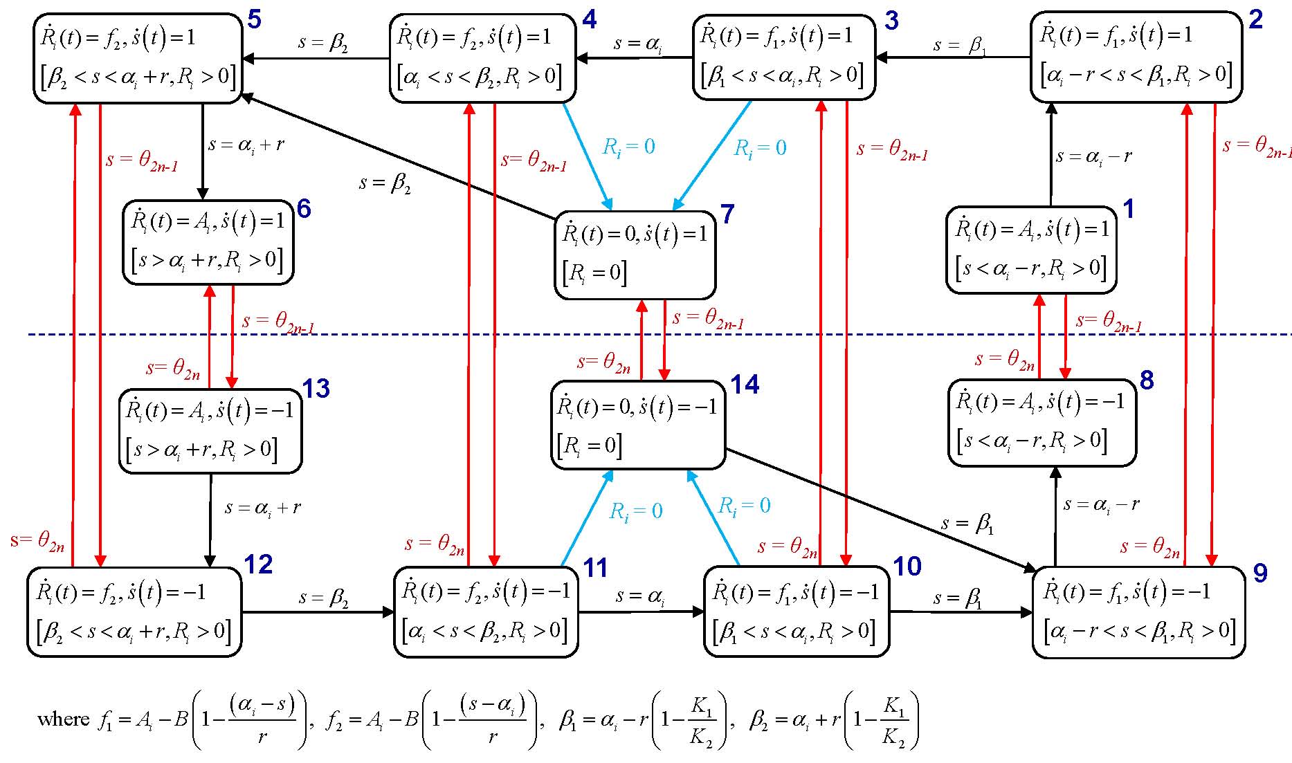
Figure 2: Hybrid automaton for each αisubscript𝛼𝑖\alpha_{i}. Red arrows represent events when the control switches between 111 and 11-1. Blue arrows represent events when Risubscript𝑅𝑖R_{i} becomes 00. Black arrows represent all other events.

We show in Fig. 2 a partial hybrid automaton model of the single-agent system where a=0𝑎0a=0 and b=L𝑏𝐿b=L. Since there is only one agent, we set s(t)=s1(t)𝑠𝑡subscript𝑠1𝑡s\left(t\right)=s_{1}\left(t\right), u(t)=u1(t)𝑢𝑡subscript𝑢1𝑡u\left(t\right)=u_{1}\left(t\right) and θ=θ1𝜃subscript𝜃1\theta=\theta_{1} for simplicity. Due to the size of the overall model, Fig. 2 is limited to the behavior of the agent with respect to a single αi,i{1,,M}subscript𝛼𝑖𝑖1𝑀\alpha_{i},i\in\{1,\ldots,M\} and ignores modes where the agent dwells on the switching points (these, however, are included in our extended analysis in Section 3.2.2.) The model consists of 14 discrete states (modes) and is symmetric in the sense that states 17171-7 correspond to the agent operating with u(t)=1𝑢𝑡1u(t)=1, and states 8148148-14 correspond to the agent operating with u(t)=1𝑢𝑡1u(t)=-1. States where u(t)=0𝑢𝑡0u\left(t\right)=0 are omitted since we do not include the waiting time parameter w=w1𝑤subscript𝑤1w=w_{1} here. The events that cause state transitions can be placed in three categories: (i)𝑖(i) The value of Ri(t)subscript𝑅𝑖𝑡R_{i}(t) becomes 0 and triggers a switch in the dynamics of (6). This can only happen when Ri(t)>0subscript𝑅𝑖𝑡0R_{i}(t)>0 and R˙i(t)=AiBpi(s(t))<0subscript˙𝑅𝑖𝑡subscript𝐴𝑖𝐵subscript𝑝𝑖𝑠𝑡0\dot{R}_{i}(t)=A_{i}-Bp_{i}(s(t))<0 (e.g., in states 333 and 444), causing a transition to state 777 in which the invariant condition is Ri(t)=0subscript𝑅𝑖𝑡0R_{i}(t)=0. (ii)𝑖𝑖(ii) The agent reaches a switching location, indicated by the guard condition s(t)=θξ𝑠𝑡subscript𝜃𝜉s(t)=\theta_{\xi} for any ξ=1,,Γ𝜉1Γ\xi=1,\ldots,\Gamma. In these cases, a transition results from a state z𝑧z to z+7𝑧7z+7 if z=1,,6𝑧16z=1,\ldots,6 and to z7𝑧7z-7 otherwise. (iii)𝑖𝑖𝑖(iii) The agent position reaches one of several critical values that affect the dynamics of Ri(t)subscript𝑅𝑖𝑡R_{i}(t) while Ri(t)>0subscript𝑅𝑖𝑡0R_{i}(t)>0. Specifically, when s(t)=αir𝑠𝑡subscript𝛼𝑖𝑟s(t)=\alpha_{i}-r, the value of pi(s(t))subscript𝑝𝑖𝑠𝑡p_{i}(s(t)) becomes strictly positive and R˙i(t)=AiBpi(s(t))>0subscript˙𝑅𝑖𝑡subscript𝐴𝑖𝐵subscript𝑝𝑖𝑠𝑡0\dot{R}_{i}(t)=A_{i}-Bp_{i}(s(t))>0, as in the transition 12121\rightarrow 2. Subsequently, when s(t)=αir(1Ai/B)𝑠𝑡subscript𝛼𝑖𝑟1subscript𝐴𝑖𝐵s(t)=\alpha_{i}-r(1-A_{i}/B), as in the transition 23232\rightarrow 3, the value of pi(s(t))subscript𝑝𝑖𝑠𝑡p_{i}(s(t)) becomes sufficiently large to cause R˙i(t)=AiBpi(s(t))<0subscript˙𝑅𝑖𝑡subscript𝐴𝑖𝐵subscript𝑝𝑖𝑠𝑡0\dot{R}_{i}(t)=A_{i}-Bp_{i}(s(t))<0 so that a transition due to Ri(t)=0subscript𝑅𝑖𝑡0R_{i}(t)=0 becomes feasible at this state. Similar transitions occur when s(t)=αi𝑠𝑡subscript𝛼𝑖s(t)=\alpha_{i}, s(t)=αi+r(1Ai/B)𝑠𝑡subscript𝛼𝑖𝑟1subscript𝐴𝑖𝐵s(t)=\alpha_{i}+r(1-A_{i}/B), and s(t)=αi+r𝑠𝑡subscript𝛼𝑖𝑟s(t)=\alpha_{i}+r. The latter results in state 666 where R˙i(t)=Ai>0subscript˙𝑅𝑖𝑡subscript𝐴𝑖0\dot{R}_{i}(t)=A_{i}>0 and the only feasible event is s(t)=θξ𝑠𝑡subscript𝜃𝜉s(t)=\theta_{\xi}, ξ𝜉\xi odd, when a switch must occur and a transition to state 131313 takes place (similarly for state 888).

IPA review. Before proceeding, we provide a brief review of the IPA framework for general stochastic hybrid systems as presented in [15]. The purpose of IPA is to study the behavior of a hybrid system state as a function of a parameter vector θΘ𝜃Θ\theta\in\Theta for a given compact, convex set ΘlΘsuperscript𝑙\Theta\subset\mathbb{R}^{l}. Let {τk(θ)}subscript𝜏𝑘𝜃\{\tau_{k}(\theta)\}, k=1,,K𝑘1𝐾k=1,\ldots,K, denote the occurrence times of all events in the state trajectory. For convenience, we set τ0=0subscript𝜏00\tau_{0}=0 and τK+1=Tsubscript𝜏𝐾1𝑇\tau_{K+1}=T. Over an interval [τk(θ),τk+1(θ))subscript𝜏𝑘𝜃subscript𝜏𝑘1𝜃[\tau_{k}(\theta),\tau_{k+1}(\theta)), the system is at some mode during which the time-driven state satisfies x˙=fk(x,θ,t)˙𝑥subscript𝑓𝑘𝑥𝜃𝑡\dot{x}\ =\ f_{k}(x,\theta,t). An event at τksubscript𝜏𝑘\tau_{k} is classified as (i)𝑖(i) Exogenous if it causes a discrete state transition independent of θ𝜃\theta and satisfies dτkdθ=0𝑑subscript𝜏𝑘𝑑𝜃0\frac{d\tau_{k}}{d\theta}=0; (ii)𝑖𝑖(ii) Endogenous, if there exists a continuously differentiable function gk:n×Θ:subscript𝑔𝑘superscript𝑛Θg_{k}:\mathbb{R}^{n}\times\Theta\rightarrow\mathbb{R} such that τk=min{t>τk1:gk(x(θ,t),θ)=0}subscript𝜏𝑘:𝑡subscript𝜏𝑘1subscript𝑔𝑘𝑥𝜃𝑡𝜃0\tau_{k}\ =\ \min\{t>\tau_{k-1}\ :\ g_{k}\left(x\left(\theta,t\right),\theta\right)=0\}; and (iii)𝑖𝑖𝑖(iii) Induced if it is triggered by the occurrence of another event at time τmτksubscript𝜏𝑚subscript𝜏𝑘\tau_{m}\leq\tau_{k}. IPA specifies how changes in θ𝜃\theta influence the state x(θ,t)𝑥𝜃𝑡x(\theta,t) and the event times τk(θ)subscript𝜏𝑘𝜃\tau_{k}(\theta) and, ultimately, how they influence interesting performance metrics which are generally expressed in terms of these variables.

Given θ=[θ1,,θΓ]𝚃𝜃superscriptsubscript𝜃1subscript𝜃Γ𝚃\theta=[\theta_{1},\ldots,\theta_{\Gamma}]^{\mathtt{T}}, we use the Jacobian matrix notation: x(t)x(θ,t)θsuperscript𝑥𝑡𝑥𝜃𝑡𝜃x^{\prime}(t)\equiv\frac{\partial x(\theta,t)}{\partial\theta}, τkτk(θ)θsuperscriptsubscript𝜏𝑘subscript𝜏𝑘𝜃𝜃\tau_{k}^{\prime}\equiv\frac{\partial\tau_{k}(\theta)}{\partial\theta}, k=1,,K𝑘1𝐾k=1,\ldots,K, for all state and event time derivatives. It is shown in [15] that x(t)superscript𝑥𝑡x^{\prime}(t) satisfies:

ddtx(t)=fk(t)xx(t)+fk(t)θ𝑑𝑑𝑡superscript𝑥𝑡subscript𝑓𝑘𝑡𝑥superscript𝑥𝑡subscript𝑓𝑘𝑡𝜃\frac{d}{dt}x^{\prime}\left(t\right)=\frac{\partial f_{k}\left(t\right)}{\partial x}x^{\prime}\left(t\right)+\frac{\partial f_{k}\left(t\right)}{\partial\theta} (27)

for t[τk,τk+1)𝑡subscript𝜏𝑘subscript𝜏𝑘1t\in[\tau_{k},\tau_{k+1}) with boundary condition:

x(τk+)=x(τk)+[fk1(τk)fk(τk+)]τksuperscript𝑥superscriptsubscript𝜏𝑘superscript𝑥superscriptsubscript𝜏𝑘delimited-[]subscript𝑓𝑘1superscriptsubscript𝜏𝑘subscript𝑓𝑘superscriptsubscript𝜏𝑘superscriptsubscript𝜏𝑘x^{\prime}(\tau_{k}^{+})\ =\ x^{\prime}(\tau_{k}^{-})+\left[f_{k-1}(\tau_{k}^{-})-f_{k}(\tau_{k}^{+})\right]\tau_{k}^{\prime} (28)

for k=0,,K𝑘0𝐾k=0,\ldots,K. In addition, in (28), the gradient vector for each τksubscript𝜏𝑘\tau_{k} is τk=0superscriptsubscript𝜏𝑘0\tau_{k}^{\prime}=0 if the event at τksubscript𝜏𝑘\tau_{k} is exogenous and

τk=[gkxfk(τk)]1(gkθ+gkxx(τk))superscriptsubscript𝜏𝑘superscriptdelimited-[]subscript𝑔𝑘𝑥subscript𝑓𝑘superscriptsubscript𝜏𝑘1subscript𝑔𝑘𝜃subscript𝑔𝑘𝑥superscript𝑥superscriptsubscript𝜏𝑘\tau_{k}^{\prime}=-\left[\frac{\partial g_{k}}{\partial x}f_{k}(\tau_{k}^{-})\right]^{-1}\left(\frac{\partial g_{k}}{\partial\theta}+\frac{\partial g_{k}}{\partial x}x^{\prime}(\tau_{k}^{-})\right) (29)

if the event at τksubscript𝜏𝑘\tau_{k} is endogenous (i.e., gk(x(θ,τk),θ)=0subscript𝑔𝑘𝑥𝜃subscript𝜏𝑘𝜃0\ g_{k}\left(x\left(\theta,\tau_{k}\right),\theta\right)=0) and defined as long as gkxfk(τk)0subscript𝑔𝑘𝑥subscript𝑓𝑘superscriptsubscript𝜏𝑘0\frac{\partial g_{k}}{\partial x}f_{k}(\tau_{k}^{-})\neq 0.

IPA equations. To clarify the presentation, we first note that i=1,,M𝑖1𝑀i=1,\ldots,M is used to index the points where uncertainty is measured; ξ=1,,Γ𝜉1Γ\xi=1,\ldots,\Gamma indexes the components of the parameter vector; and k=1,,K𝑘1𝐾k=1,\ldots,K indexes event times. In order to apply the three fundamental IPA equations (27)-(29) to our system, we use the state vector x(t)=[s(t),R1(t),,RM(t)]𝚃𝑥𝑡superscript𝑠𝑡subscript𝑅1𝑡subscript𝑅𝑀𝑡𝚃x\left(t\right)=[s\left(t\right),R_{1}(t),\ldots,R_{M}(t)]^{\mathtt{T}} and parameter vector θ=[θ1,,θΓ]𝚃𝜃superscriptsubscript𝜃1subscript𝜃Γ𝚃\theta=[\theta_{1},\ldots,\theta_{\Gamma}]^{\mathtt{T}}. We then identify all events that can occur in Fig. 2 and consider intervals [τk(θ),τk+1(θ))subscript𝜏𝑘𝜃subscript𝜏𝑘1𝜃[\tau_{k}(\theta),\tau_{k+1}(\theta)) over which the system is in one of the 14 states shown for each i=1,,M𝑖1𝑀i=1,\ldots,M. Applying (27) to s(t)𝑠𝑡s(t) with fk(t)=1subscript𝑓𝑘𝑡1f_{k}\left(t\right)=1 or 11-1 due to (1) and (12), the solution yields the gradient vector s(t)=[sθ1(t),,sθM(t)]𝚃𝑠𝑡superscript𝑠subscript𝜃1𝑡𝑠subscript𝜃𝑀𝑡𝚃\nabla s(t)=[\frac{\partial s}{\partial\theta_{1}}(t),\ldots,\frac{\partial s}{\partial\theta_{M}}(t)]^{\mathtt{T}}, where

sθξ(t)=sθξ(τk+), for t[τk,τk+1)formulae-sequence𝑠subscript𝜃𝜉𝑡𝑠subscript𝜃𝜉superscriptsubscript𝜏𝑘 for 𝑡subscript𝜏𝑘subscript𝜏𝑘1\frac{\partial s}{\partial\theta_{\xi}}(t)=\frac{\partial s}{\partial\theta_{\xi}}(\tau_{k}^{+}),\text{ for }t\in[\tau_{k},\tau_{k+1}) (30)

for all k=1,,K𝑘1𝐾k=1,\ldots,K, i.e., for all states z(t){1,,14}𝑧𝑡114z(t)\in\{1,\ldots,14\}. Similarly, let Ri(t)=[Riθ1(t),,RiθM(t)]𝚃subscript𝑅𝑖𝑡superscriptsubscript𝑅𝑖subscript𝜃1𝑡subscript𝑅𝑖subscript𝜃𝑀𝑡𝚃\nabla R_{i}(t)=[\frac{\partial R_{i}}{\partial\theta_{1}}(t),\ldots,\frac{\partial R_{i}}{\partial\theta_{M}}(t)]^{\mathtt{T}} for i=1,,M𝑖1𝑀i=1,\ldots,M. We note from (6) that fk(t)=0subscript𝑓𝑘𝑡0f_{k}\left(t\right)=0 for states z(t)Z1{7,14}𝑧𝑡subscript𝑍1714z(t)\in Z_{1}\equiv\{7,14\}; fk(t)=Aisubscript𝑓𝑘𝑡subscript𝐴𝑖f_{k}\left(t\right)=A_{i} for states z(t)Z2{1,6,8,13}𝑧𝑡subscript𝑍216813z(t)\in Z_{2}\equiv\{1,6,8,13\}; and fk(t)=AiBpi(s(t))subscript𝑓𝑘𝑡subscript𝐴𝑖𝐵subscript𝑝𝑖𝑠𝑡f_{k}\left(t\right)=A_{i}-Bp_{i}(s(t)) for all other states which we further classify into Z3{2,3,11,12}subscript𝑍3231112Z_{3}\equiv\{2,3,11,12\} and Z4{4,5,9,10}subscript𝑍445910Z_{4}\equiv\{4,5,9,10\}. Thus, solving (27) and using (30) gives:

Ri(t)=Ri(τk+){0if z(t)Z1Z2B(pi(s)s)s(τk+)(tτk)otherwisesubscript𝑅𝑖𝑡subscript𝑅𝑖superscriptsubscript𝜏𝑘cases0if 𝑧𝑡subscript𝑍1subscript𝑍2𝐵subscript𝑝𝑖𝑠𝑠𝑠superscriptsubscript𝜏𝑘𝑡subscript𝜏𝑘otherwise\nabla R_{i}\left(t\right)=\nabla R_{i}(\tau_{k}^{+})-\left\{\begin{array}[c]{ll}0&\text{if }z\left(t\right)\in Z_{1}\cup Z_{2}\\ B\left(\frac{\partial p_{i}(s)}{\partial s}\right)\nabla s\left(\tau_{k}^{+}\right)\cdot(t-\tau_{k})&\text{otherwise}\end{array}\right.

where pi(s)s=±1rsubscript𝑝𝑖𝑠𝑠plus-or-minus1𝑟\frac{\partial p_{i}(s)}{\partial s}=\pm\frac{1}{r} as evaluated from (4) depending on the sign of αis(t)subscript𝛼𝑖𝑠𝑡\alpha_{i}-s(t) at each associated automaton state.

We now turn our attention to the determination of s(τk+)𝑠superscriptsubscript𝜏𝑘\nabla s\left(\tau_{k}^{+}\right) and Ri(τk+)subscript𝑅𝑖superscriptsubscript𝜏𝑘\nabla R_{i}(\tau_{k}^{+}) which are needed to evaluate Ri(t)subscript𝑅𝑖𝑡\nabla R_{i}\left(t\right) above. To do so, we use (28), which involves the event time gradient vectors τk=[τkθ1,,τkθΓ]𝚃subscript𝜏𝑘superscriptsubscript𝜏𝑘subscript𝜃1subscript𝜏𝑘subscript𝜃Γ𝚃\nabla\tau_{k}=[\frac{\partial\tau_{k}}{\partial\theta_{1}},\ldots,\frac{\partial\tau_{k}}{\partial\theta_{\Gamma}}]^{\mathtt{T}} for k=1,,K𝑘1𝐾k=1,\ldots,K (the value of K𝐾K depends on T𝑇T.) Looking at Fig. 2, there are three readily distinguishable cases regarding the events that cause discrete state transitions:

Case 1: An event at time τksubscript𝜏𝑘\tau_{k} which is neither Ri=0subscript𝑅𝑖0R_{i}=0 nor s=θξ𝑠subscript𝜃𝜉s=\theta_{\xi}, for any ξ=1,,Γ𝜉1Γ\xi=1,\ldots,\Gamma. In this case, it is easy to see that the dynamics of both s(t)𝑠𝑡s(t) and Ri(t)subscript𝑅𝑖𝑡R_{i}(t) are continuous, so that fk1(τk)=fk(τk+)subscript𝑓𝑘1superscriptsubscript𝜏𝑘subscript𝑓𝑘superscriptsubscript𝜏𝑘f_{k-1}(\tau_{k}^{-})=f_{k}(\tau_{k}^{+}) in (28) applied to s(t)𝑠𝑡s\left(t\right) and Ri(t),subscript𝑅𝑖𝑡R_{i}(t), i=1,,M𝑖1𝑀i=1,\ldots,M gives:

{s(τk+)=s(τk)Ri(τk+)=Ri(τk), i=1,,Mcases𝑠superscriptsubscript𝜏𝑘𝑠superscriptsubscript𝜏𝑘formulae-sequencesubscript𝑅𝑖superscriptsubscript𝜏𝑘subscript𝑅𝑖superscriptsubscript𝜏𝑘 𝑖1𝑀\left\{\begin{array}[c]{l}\nabla s\left(\tau_{k}^{+}\right)=\nabla s\left(\tau_{k}^{-}\right)\\ \nabla R_{i}(\tau_{k}^{+})=\nabla R_{i}(\tau_{k}^{-}),\text{ \ }i=1,\ldots,M\end{array}\right. (31)

Case 2: An event Ri=0subscript𝑅𝑖0R_{i}=0 at time τksubscript𝜏𝑘\tau_{k}. This corresponds to transitions 37373\rightarrow 7, 47474\rightarrow 7, 1014101410\rightarrow 14 and 1114111411\rightarrow 14 in Fig. 2 where the dynamics of s(t)𝑠𝑡s(t) are still continuous, but the dynamics of Ri(t)subscript𝑅𝑖𝑡R_{i}(t) switch from fk1(τk)=AiBpi(s(τk))subscript𝑓𝑘1superscriptsubscript𝜏𝑘subscript𝐴𝑖𝐵subscript𝑝𝑖𝑠superscriptsubscript𝜏𝑘f_{k-1}(\tau_{k}^{-})=A_{i}-Bp_{i}(s(\tau_{k}^{-})) to fk(τk+)=0subscript𝑓𝑘superscriptsubscript𝜏𝑘0f_{k}(\tau_{k}^{+})=0. Thus, s(τk)=s(τk+)𝑠superscriptsubscript𝜏𝑘𝑠superscriptsubscript𝜏𝑘\nabla s\left(\tau_{k}^{-}\right)=\nabla s\left(\tau_{k}^{+}\right), but we need to evaluate τksuperscriptsubscript𝜏𝑘\tau_{k}^{\prime} to determine Ri(τk+)subscript𝑅𝑖superscriptsubscript𝜏𝑘\nabla R_{i}(\tau_{k}^{+}). Observing that this event is endogenous, (29) applies with gk=Ri=0subscript𝑔𝑘subscript𝑅𝑖0g_{k}=R_{i}=0 and we get

τkθξ=Riθξ(τk)AiBpi(s(τk)), ξ=1,,Γ, k=1,,Kformulae-sequencesubscript𝜏𝑘subscript𝜃𝜉subscript𝑅𝑖subscript𝜃𝜉superscriptsubscript𝜏𝑘subscript𝐴𝑖𝐵subscript𝑝𝑖𝑠superscriptsubscript𝜏𝑘formulae-sequence 𝜉1Γ 𝑘1𝐾\frac{\partial\tau_{k}}{\partial\theta_{\xi}}=-\frac{\frac{\partial R_{i}}{\partial\theta_{\xi}}\left(\tau_{k}^{-}\right)}{A_{i}-Bp_{i}(s(\tau_{k}^{-}))},\text{ \ \ }\xi=1,\ldots,\Gamma,\text{ }k=1,\ldots,K

It follows from (28) that

Riθξ(τk+)=Riθξ(τk)[AiBpi(s(τk))]Riθξ(τk)AiBpi(s(τk))=0subscript𝑅𝑖subscript𝜃𝜉superscriptsubscript𝜏𝑘subscript𝑅𝑖subscript𝜃𝜉superscriptsubscript𝜏𝑘delimited-[]subscript𝐴𝑖𝐵subscript𝑝𝑖𝑠superscriptsubscript𝜏𝑘subscript𝑅𝑖subscript𝜃𝜉superscriptsubscript𝜏𝑘subscript𝐴𝑖𝐵subscript𝑝𝑖𝑠superscriptsubscript𝜏𝑘0\frac{\partial R_{i}}{\partial\theta_{\xi}}\left(\tau_{k}^{+}\right)=\frac{\partial R_{i}}{\partial\theta_{\xi}}\left(\tau_{k}^{-}\right)-\frac{[A_{i}-Bp_{i}(s(\tau_{k}^{-}))]\frac{\partial R_{i}}{\partial\theta_{\xi}}\left(\tau_{k}^{-}\right)}{A_{i}-Bp_{i}(s(\tau_{k}^{-}))}=0

Thus, whenever an event occurs at τksubscript𝜏𝑘\tau_{k} such that Ri(τk)subscript𝑅𝑖subscript𝜏𝑘R_{i}(\tau_{k}) becomes zero, Riθξ(τk+)subscript𝑅𝑖subscript𝜃𝜉superscriptsubscript𝜏𝑘\frac{\partial R_{i}}{\partial\theta_{\xi}}\left(\tau_{k}^{+}\right) is always reset to 00 regardless of Riθξ(τk)subscript𝑅𝑖subscript𝜃𝜉superscriptsubscript𝜏𝑘\frac{\partial R_{i}}{\partial\theta_{\xi}}\left(\tau_{k}^{-}\right).

Case 3: An event at time τksubscript𝜏𝑘\tau_{k} due to a control sign change at s=θξ𝑠subscript𝜃𝜉s=\theta_{\xi}, ξ=1,,Γ𝜉1Γ\xi=1,\ldots,\Gamma. This corresponds to any transition between the upper and lower part of the hybrid automaton in Fig. 2. In this case, the dynamics of Ri(t)subscript𝑅𝑖𝑡R_{i}(t) are continuous and we have Riθξ(τk+)=Riθξ(τk)subscript𝑅𝑖subscript𝜃𝜉superscriptsubscript𝜏𝑘subscript𝑅𝑖subscript𝜃𝜉superscriptsubscript𝜏𝑘\frac{\partial R_{i}}{\partial\theta_{\xi}}\left(\tau_{k}^{+}\right)=\frac{\partial R_{i}}{\partial\theta_{\xi}}\left(\tau_{k}^{-}\right) for all i,ξ,k𝑖𝜉𝑘i,\xi,k. On the other hand, we have s˙(τk+)=u(τk+)=u(τk)=±1˙𝑠superscriptsubscript𝜏𝑘𝑢superscriptsubscript𝜏𝑘𝑢superscriptsubscript𝜏𝑘plus-or-minus1\dot{s}(\tau_{k}^{+})=u(\tau_{k}^{+})=-u(\tau_{k}^{-})=\pm 1. Observing that any such event is endogenous, (29) applies with gk=sθξ=0subscript𝑔𝑘𝑠subscript𝜃𝜉0g_{k}=s-\theta_{\xi}=0 for some ξ=1,,Γ𝜉1Γ\xi=1,\ldots,\Gamma and we get

τkθξ=1sθξ(τk)u(τk)subscript𝜏𝑘subscript𝜃𝜉1𝑠subscript𝜃𝜉superscriptsubscript𝜏𝑘𝑢superscriptsubscript𝜏𝑘\frac{\partial\tau_{k}}{\partial\theta_{\xi}}=\frac{1-\frac{\partial s}{\partial\theta_{\xi}}\left(\tau_{k}^{-}\right)}{u(\tau_{k}^{-})} (32)

Combining (32) with (28) and recalling that u(τk+)=u(τk)𝑢superscriptsubscript𝜏𝑘𝑢superscriptsubscript𝜏𝑘u(\tau_{k}^{+})=-u(\tau_{k}^{-}), we have

sθξ(τk+)=sθξ(τk)+[u(τk)u(τk+)]1sθξ(τk)u(τk)=2𝑠subscript𝜃𝜉superscriptsubscript𝜏𝑘𝑠subscript𝜃𝜉superscriptsubscript𝜏𝑘delimited-[]𝑢superscriptsubscript𝜏𝑘𝑢superscriptsubscript𝜏𝑘1𝑠subscript𝜃𝜉superscriptsubscript𝜏𝑘𝑢superscriptsubscript𝜏𝑘2\frac{\partial s}{\partial\theta_{\xi}}(\tau_{k}^{+})=\ \frac{\partial s}{\partial\theta_{\xi}}(\tau_{k}^{-})+[u\left(\tau_{k}^{-}\right)-u(\tau_{k}^{+})]\frac{1-\frac{\partial s}{\partial\theta_{\xi}}\left(\tau_{k}^{-}\right)}{u(\tau_{k}^{-})}=2

where sθξ(τk)=0𝑠subscript𝜃𝜉superscriptsubscript𝜏𝑘0\frac{\partial s}{\partial\theta_{\xi}}\left(\tau_{k}^{-}\right)=0 because sθξ(0)=0=sθξ(t)𝑠subscript𝜃𝜉00𝑠subscript𝜃𝜉𝑡\frac{\partial s}{\partial\theta_{\xi}}\left(0\right)=0=\frac{\partial s}{\partial\theta_{\xi}}\left(t\right) for all t[0,τk)𝑡0subscript𝜏𝑘t\in[0,\tau_{k}), since the position of the agent cannot be affected by θξsubscript𝜃𝜉\theta_{\xi} prior to this event.

In this case, we also need to consider the effect of perturbations to θjsubscript𝜃𝑗\theta_{j} for j<ξ𝑗𝜉j<\xi, i.e., prior to the current event time τksubscript𝜏𝑘\tau_{k} (clearly, for j>ξ𝑗𝜉j>\xi, sθj(τk+)=0𝑠subscript𝜃𝑗superscriptsubscript𝜏𝑘0\frac{\partial s}{\partial\theta_{j}}(\tau_{k}^{+})=0 since the current position of the agent cannot be affected by future events.) Observe that since gk=sθξ=0subscript𝑔𝑘𝑠subscript𝜃𝜉0g_{k}=s-\theta_{\xi}=0, we have gkθj=0subscript𝑔𝑘subscript𝜃𝑗0\frac{\partial g_{k}}{\partial\theta_{j}}=0 for jξ𝑗𝜉j\neq\xi and (29) gives

τkθj=sθj(τk)u(τk)subscript𝜏𝑘subscript𝜃𝑗𝑠subscript𝜃𝑗superscriptsubscript𝜏𝑘𝑢superscriptsubscript𝜏𝑘\frac{\partial\tau_{k}}{\partial\theta_{j}}=-\frac{\frac{\partial s}{\partial\theta_{j}}\left(\tau_{k}^{-}\right)}{u(\tau_{k}^{-})}

so that using this in (28) we get:

sθj(τk+)=sθj(τk)[u(τk)u(τk+)]sθj(τk)u(τk)=sθj(τk)𝑠subscript𝜃𝑗superscriptsubscript𝜏𝑘𝑠subscript𝜃𝑗superscriptsubscript𝜏𝑘delimited-[]𝑢superscriptsubscript𝜏𝑘𝑢superscriptsubscript𝜏𝑘𝑠subscript𝜃𝑗superscriptsubscript𝜏𝑘𝑢superscriptsubscript𝜏𝑘𝑠subscript𝜃𝑗superscriptsubscript𝜏𝑘\frac{\partial s}{\partial\theta_{j}}(\tau_{k}^{+})=\frac{\partial s}{\partial\theta_{j}}(\tau_{k}^{-})-\frac{\left[u\left(\tau_{k}^{-}\right)-u(\tau_{k}^{+})\right]\frac{\partial s}{\partial\theta_{j}}\left(\tau_{k}^{-}\right)}{u\left(\tau_{k}^{-}\right)}=-\frac{\partial s}{\partial\theta_{j}}\left(\tau_{k}^{-}\right)

Combining the above results, the components of s(τk+)𝑠superscriptsubscript𝜏𝑘\nabla s(\tau_{k}^{+}) where τksubscript𝜏𝑘\tau_{k} is the event time when s(τk)=θξ𝑠subscript𝜏𝑘subscript𝜃𝜉s(\tau_{k})=\theta_{\xi} for some ξ𝜉\xi, are given by

sθj(τk+)={sθj(τk)if j=1,,ξ12if j=ξ0if j>ξ𝑠subscript𝜃𝑗superscriptsubscript𝜏𝑘cases𝑠subscript𝜃𝑗superscriptsubscript𝜏𝑘if 𝑗1𝜉12if 𝑗𝜉0if 𝑗𝜉\frac{\partial s}{\partial\theta_{j}}(\tau_{k}^{+})\ =\left\{\begin{array}[c]{ll}-\frac{\partial s}{\partial\theta_{j}}\left(\tau_{k}^{-}\right)&\text{if }j=1,\ldots,\xi-1\\ 2&\text{if }j=\xi\\ 0&\text{if }j>\xi\end{array}\right. (33)

It follows from (30) and the analysis of all three cases above that sθξ(t)𝑠subscript𝜃𝜉𝑡\frac{\partial s}{\partial\theta_{\xi}}\left(t\right) for all ξ𝜉\xi is constant throughout an optimal trajectory except at transitions caused by control switching locations (Case 3). In particular, for the k𝑘kth event corresponding to s(τk)=θξ𝑠subscript𝜏𝑘subscript𝜃𝜉s(\tau_{k})=\theta_{\xi}, t[τk,T]𝑡subscript𝜏𝑘𝑇t\in[\tau_{k},T], if u(t)=1𝑢𝑡1u\left(t\right)=1, then sθξ(t)=2𝑠subscript𝜃𝜉𝑡2\frac{\partial s}{\partial\theta_{\xi}}\left(t\right)=-2 if ξ𝜉\xi is odd, and sθξ(t)=2𝑠subscript𝜃𝜉𝑡2\frac{\partial s}{\partial\theta_{\xi}}\left(t\right)=2 if ξ𝜉\xi is even; similarly, if u(t)=1𝑢𝑡1u\left(t\right)=-1, then sθξ(t)=2𝑠subscript𝜃𝜉𝑡2\frac{\partial s}{\partial\theta_{\xi}}\left(t\right)=2 if ξ𝜉\xi is odd and sθξ(t)=2𝑠subscript𝜃𝜉𝑡2\frac{\partial s}{\partial\theta_{\xi}}\left(t\right)=-2 if ξ𝜉\xi is even. In summary, we can write:

sθξ(t)={(1)ξ2u(t)tτk0t<τkξ=1,,Γformulae-sequence𝑠subscript𝜃𝜉𝑡casessuperscript1𝜉2𝑢𝑡𝑡subscript𝜏𝑘0𝑡subscript𝜏𝑘𝜉1Γ\frac{\partial s}{\partial\theta_{\xi}}\left(t\right)=\left\{\begin{array}[c]{cc}\left(-1\right)^{\xi}\cdot 2u\left(t\right)&t\geq\tau_{k}\\ 0&t<\tau_{k}\end{array}\right.\text{, \ }\xi=1,\ldots,\Gamma (34)

Finally, we can combine (34) with our results for Riθξ(t)subscript𝑅𝑖subscript𝜃𝜉𝑡\frac{\partial R_{i}}{\partial\theta_{\xi}}\left(t\right) in all three cases above. Letting s(τl)=θξ𝑠subscript𝜏𝑙subscript𝜃𝜉s(\tau_{l})=\theta_{\xi}, we obtain the following expression for Riθξ(t)subscript𝑅𝑖subscript𝜃𝜉𝑡\frac{\partial R_{i}}{\partial\theta_{\xi}}\left(t\right) for all kl,𝑘𝑙k\geq l, t[τk,τk+1)𝑡subscript𝜏𝑘subscript𝜏𝑘1t\in[\tau_{k},\tau_{k+1}):

Riθξ(t)=Riθξ(τk+)+{0if z(t)Z1Z2(1)ξ+12Bru(τk+)(tτk)if z(t)Z3(1)ξ+12Bru(τk+)(tτk)if z(t)Z4subscript𝑅𝑖subscript𝜃𝜉𝑡subscript𝑅𝑖subscript𝜃𝜉superscriptsubscript𝜏𝑘cases0if 𝑧𝑡subscript𝑍1subscript𝑍2superscript1𝜉12𝐵𝑟𝑢superscriptsubscript𝜏𝑘𝑡subscript𝜏𝑘if 𝑧𝑡subscript𝑍3superscript1𝜉12𝐵𝑟𝑢superscriptsubscript𝜏𝑘𝑡subscript𝜏𝑘if 𝑧𝑡subscript𝑍4\frac{\partial R_{i}}{\partial\theta_{\xi}}\left(t\right)=\frac{\partial R_{i}}{\partial\theta_{\xi}}\left(\tau_{k}^{+}\right)+\left\{\begin{array}[c]{cl}0&\text{if }z(t)\in Z_{1}\cup Z_{2}\\ \left(-1\right)^{\xi+1}\frac{2B}{r}u\left(\tau_{k}^{+}\right)\cdot(t-\tau_{k})&\text{if }z(t)\in Z_{3}\\ -\left(-1\right)^{\xi+1}\frac{2B}{r}u\left(\tau_{k}^{+}\right)\cdot(t-\tau_{k})&\text{if }z(t)\in Z_{4}\end{array}\right. (35)

with boundary condition

Riθξ(τk+)={0if z(τk+)Z1Riθξ(τk)otherwisesubscript𝑅𝑖subscript𝜃𝜉superscriptsubscript𝜏𝑘cases0if 𝑧superscriptsubscript𝜏𝑘subscript𝑍1subscript𝑅𝑖subscript𝜃𝜉superscriptsubscript𝜏𝑘otherwise\frac{\partial R_{i}}{\partial\theta_{\xi}}(\tau_{k}^{+})=\left\{\begin{array}[c]{cl}0&\text{if }z\left(\tau_{k}^{+}\right)\in Z_{1}\\ \frac{\partial R_{i}}{\partial\theta_{\xi}}(\tau_{k}^{-})&\text{otherwise}\end{array}\right. (36)

Objective Function Gradient Evaluation. Based on our analysis, the objective function (7) in problem P1 can now be written as J(θ)𝐽𝜃J(\theta), a function of θ𝜃\theta instead of u(t)𝑢𝑡u\left(t\right) and we can rewrite it as

J(θ)=1Ti=1Mk=0Kτk(θ)τk+1(θ)Ri(t,θ)𝑑t𝐽𝜃1𝑇superscriptsubscript𝑖1𝑀superscriptsubscript𝑘0𝐾superscriptsubscriptsubscript𝜏𝑘𝜃subscript𝜏𝑘1𝜃subscript𝑅𝑖𝑡𝜃differential-d𝑡J(\theta)=\frac{1}{T}\sum_{i=1}^{M}\sum_{k=0}^{K}{\displaystyle\int_{\tau_{k}(\theta)}^{\tau_{k+1}(\theta)}}R_{i}\left(t,\theta\right)dt

where we have explicitly indicated the dependence on θ𝜃\theta. We then obtain:

J(θ)=1Ti=1Mk=0K(τkτk+1Ri(t)𝑑t+Ri(τk+1)τk+1Ri(τk)τk)𝐽𝜃1𝑇superscriptsubscript𝑖1𝑀superscriptsubscript𝑘0𝐾superscriptsubscriptsubscript𝜏𝑘subscript𝜏𝑘1subscript𝑅𝑖𝑡differential-d𝑡subscript𝑅𝑖subscript𝜏𝑘1subscript𝜏𝑘1subscript𝑅𝑖subscript𝜏𝑘subscript𝜏𝑘\nabla J(\theta)=\frac{1}{T}{\displaystyle\sum_{i=1}^{M}}{\displaystyle\sum_{k=0}^{K}}\left({\displaystyle\int_{\tau_{k}}^{\tau_{k+1}}}\nabla R_{i}\left(t\right)dt+R_{i}\left(\tau_{k+1}\right)\nabla\tau_{k+1}-R_{i}\left(\tau_{k}\right)\nabla\tau_{k}\right)

Observing the cancelation of all terms of the form Ri(τk)τksubscript𝑅𝑖subscript𝜏𝑘subscript𝜏𝑘R_{i}\left(\tau_{k}\right)\nabla\tau_{k} for all k𝑘k (with τ0=0subscript𝜏00\tau_{0}=0, τK+1=Tsubscript𝜏𝐾1𝑇\tau_{K+1}=T fixed), we finally get

J(θ)=1Ti=1Mk=0Kτk(θ)τk+1(θ)Ri(t)𝑑t.𝐽𝜃1𝑇superscriptsubscript𝑖1𝑀superscriptsubscript𝑘0𝐾superscriptsubscriptsubscript𝜏𝑘𝜃subscript𝜏𝑘1𝜃subscript𝑅𝑖𝑡differential-d𝑡\nabla J(\theta)=\frac{1}{T}{\displaystyle\sum_{i=1}^{M}}{\displaystyle\sum_{k=0}^{K}}{\displaystyle\int_{\tau_{k}(\theta)}^{\tau_{k+1}(\theta)}}\nabla R_{i}\left(t\right)dt. (37)

The evaluation of J(θ)𝐽𝜃\nabla J(\theta) therefore depends entirely on Ri(t)subscript𝑅𝑖𝑡\nabla R_{i}\left(t\right), which is obtained from (35)-(36) and the event times τksubscript𝜏𝑘\tau_{k}, k=1,,K𝑘1𝐾k=1,\ldots,K, given initial conditions s(0)=0𝑠00s\left(0\right)=0, Ri(0)subscript𝑅𝑖0R_{i}\left(0\right) for i=1,,M𝑖1𝑀i=1,\ldots,M and Ri(0)=0subscript𝑅𝑖00\nabla R_{i}(0)=0. Since Ri(t)subscript𝑅𝑖𝑡\nabla R_{i}\left(t\right) itself depends only on the event times τksubscript𝜏𝑘\tau_{k}, k=1,,K𝑘1𝐾k=1,\ldots,K, the gradient J(θ)𝐽𝜃\nabla J(\theta) is obtained by observing the switching times in a trajectory over [0,T]0𝑇[0,T] characterized by the vector θ𝜃\theta.

3.2.2 Multi agent solution where a0𝑎0a\geq 0 and bL𝑏𝐿b\leq L

Next, we extend the results obtained in the previous section to the general multi-agent problem where we also allow a0𝑎0a\geq 0 and bL𝑏𝐿b\leq L. Recall that we require 0arn0𝑎subscript𝑟𝑛0\leq a\leq r_{n} and LrmbL𝐿subscript𝑟𝑚𝑏𝐿L-r_{m}\leq b\leq L, for at least some n,m=1,,Nformulae-sequence𝑛𝑚1𝑁n,m=1,\ldots,N since, otherwise, controlling agent movement cannot affect Ri(t)subscript𝑅𝑖𝑡R_{i}(t) for all αisubscript𝛼𝑖\alpha_{i} located outside the sensing range of agents. We now include both parameter vectors θn=[θn,1,,θn,Γn]𝚃subscript𝜃𝑛superscriptsubscript𝜃𝑛1subscript𝜃𝑛subscriptΓ𝑛𝚃\theta_{n}=[\theta_{n,1},\ldots,\theta_{n,\Gamma_{n}}]^{\mathtt{T}} and wn=[wn,1,wn,Γn]Tsubscript𝑤𝑛superscriptsubscript𝑤𝑛1subscript𝑤𝑛subscriptΓ𝑛Tw_{n}=[w_{n,1},\ldots w_{n,\Gamma_{n}}]^{\text{T}} for each agent n𝑛n and, for notational simplicity, concatenate them to construct θ=[θ1,,θN]𝚃𝜃superscriptsubscript𝜃1subscript𝜃𝑁𝚃\theta=\left[\theta_{1},\ldots,\theta_{N}\right]^{\mathtt{T}} and w=[w1,,wN]𝚃𝑤superscriptsubscript𝑤1subscript𝑤𝑁𝚃w=\left[w_{1},\ldots,w_{N}\right]^{\mathtt{T}}. The solution of problem P1 reduces to the determination of optimal parameter vectors θsuperscript𝜃\theta^{\star} and wsuperscript𝑤w^{\ast} and we will use IPA to evaluate J(θ,w)=[dJ(θ,w)dθdJ(θ,w)dw]𝚃𝐽𝜃𝑤superscriptdelimited-[]𝑑𝐽𝜃𝑤𝑑𝜃𝑑𝐽𝜃𝑤𝑑𝑤𝚃\nabla J(\theta,w)=[\frac{dJ\left(\theta,w\right)}{d\theta}\frac{dJ\left(\theta,w\right)}{dw}]^{\mathtt{T}}. Similar to (37), it is clear that this depends on Ri(t)=[Ri(t)θRi(t)w]𝚃subscript𝑅𝑖𝑡superscriptdelimited-[]subscript𝑅𝑖𝑡𝜃subscript𝑅𝑖𝑡𝑤𝚃\nabla R_{i}(t)=\left[\frac{\partial R_{i}\left(t\right)}{\partial\theta}\frac{\partial R_{i}\left(t\right)}{\partial w}\right]^{\mathtt{T}} and the event times τksubscript𝜏𝑘\tau_{k}, k=1,,K,𝑘1𝐾k=1,\ldots,K, observed on a trajectory over [0,T]0𝑇[0,T] with given θ𝜃\theta and w𝑤w.

IPA equations. We begin by recalling the dynamics of Ri(t)subscript𝑅𝑖𝑡R_{i}\left(t\right) in (6) which depend on the relative positions of all agents with respect to αisubscript𝛼𝑖\alpha_{i} and change at time instants τksubscript𝜏𝑘\tau_{k} such that either Ri(τk)=0subscript𝑅𝑖subscript𝜏𝑘0R_{i}(\tau_{k})=0 with Ri(τk)>0subscript𝑅𝑖superscriptsubscript𝜏𝑘0R_{i}(\tau_{k}^{-})>0 or Ai>BPi(𝐬(τk))subscript𝐴𝑖𝐵subscript𝑃𝑖𝐬subscript𝜏𝑘A_{i}>BP_{i}\left(\mathbf{s}(\tau_{k})\right) with Ri(τk)=0subscript𝑅𝑖superscriptsubscript𝜏𝑘0R_{i}(\tau_{k}^{-})=0. Moreover, using (1) and our analysis in Section 3.1, the dynamics of sn(t)subscript𝑠𝑛𝑡s_{n}\left(t\right), n=1,,N𝑛1𝑁n=1,\ldots,N, in an optimal trajectory can be expressed as follows. Define Θn,ξ=(θn,ξ1,θn,ξ)subscriptΘ𝑛𝜉subscript𝜃𝑛𝜉1subscript𝜃𝑛𝜉\Theta_{n,\xi}=(\theta_{n,\xi-1},\theta_{n,\xi}) if ξ𝜉\xi is odd and Θn,ξ=(θn,ξ,θn,ξ1)subscriptΘ𝑛𝜉subscript𝜃𝑛𝜉subscript𝜃𝑛𝜉1\Theta_{n,\xi}=(\theta_{n,\xi},\theta_{n,\xi-1}) if ξ𝜉\xi is even to be the ξ𝜉\xith interval between successive switching points for any n=1,,N𝑛1𝑁n=1,\ldots,N, where θn,0=sn(0)subscript𝜃𝑛0subscript𝑠𝑛0\theta_{n,0}=s_{n}(0). Then, for ξ=1,2,𝜉12\xi=1,2,\ldots,

s˙n(t)={1sn(t)Θn,ξ, ξ odd1sn(t)Θn,ξ, ξ even0otherwisesubscript˙𝑠𝑛𝑡cases1subscript𝑠𝑛𝑡subscriptΘ𝑛𝜉 𝜉 odd1subscript𝑠𝑛𝑡subscriptΘ𝑛𝜉 𝜉 even0otherwise\dot{s}_{n}\left(t\right)=\left\{\begin{array}[c]{ll}1&s_{n}(t)\in\Theta_{n,\xi},\text{ }\xi\text{ odd}\\ -1&s_{n}(t)\in\Theta_{n,\xi},\text{ }\xi\text{ even}\\ 0&\text{otherwise}\end{array}\right. (38)

where transitions for sn(t)subscript𝑠𝑛𝑡s_{n}\left(t\right) from ±1plus-or-minus1\pm 1 to 1minus-or-plus1\mp 1 are incorporated by treating them as cases where wn,ξ=0subscript𝑤𝑛𝜉0w_{n,\xi}=0, i.e., no dwelling at a switching point θn,ξsubscript𝜃𝑛𝜉\theta_{n,\xi} (in which case s˙n(t)=0subscript˙𝑠𝑛𝑡0\dot{s}_{n}\left(t\right)=0.) We can now concentrate on all events causing switches either in the dynamics of any Ri(t)subscript𝑅𝑖𝑡R_{i}\left(t\right), i=1,,M𝑖1𝑀i=1,\ldots,M, or the dynamics of any sn(t)subscript𝑠𝑛𝑡s_{n}(t), n=1,,N𝑛1𝑁n=1,\ldots,N. From (28), any other event at some time τksubscript𝜏𝑘\tau_{k} in this hybrid system cannot modify the values of Ri(t)=[Ri(t)θRi(t)w]𝚃subscript𝑅𝑖𝑡superscriptdelimited-[]subscript𝑅𝑖𝑡𝜃subscript𝑅𝑖𝑡𝑤𝚃\nabla R_{i}(t)=\left[\frac{\partial R_{i}\left(t\right)}{\partial\theta}\frac{\partial R_{i}\left(t\right)}{\partial w}\right]^{\mathtt{T}} or sn(t)=[sn(t)θnsn(t)wn]𝚃subscript𝑠𝑛𝑡superscriptdelimited-[]subscript𝑠𝑛𝑡subscript𝜃𝑛subscript𝑠𝑛𝑡subscript𝑤𝑛𝚃\nabla s_{n}(t)=\left[\frac{\partial s_{n}\left(t\right)}{\partial\theta_{n}}\frac{\partial s_{n}\left(t\right)}{\partial w_{n}}\right]^{\mathtt{T}} at t=τk𝑡subscript𝜏𝑘t=\tau_{k}.

First, applying (27) to sn(t)subscript𝑠𝑛𝑡s_{n}(t) with fk(t)=1subscript𝑓𝑘𝑡1f_{k}\left(t\right)=1, 11-1 or 00 due to (38), the solution yields

sn(t)=sn(τk+), for t[τk,τk+1)formulae-sequencesubscript𝑠𝑛𝑡subscript𝑠𝑛superscriptsubscript𝜏𝑘 for 𝑡subscript𝜏𝑘subscript𝜏𝑘1\nabla s_{n}(t)=\nabla s_{n}(\tau_{k}^{+}),\text{ for }t\in[\tau_{k},\tau_{k+1}) (39)

for all k=1,,K𝑘1𝐾k=1,\ldots,K, n=𝑛absentn= 1,,N.1𝑁1,\ldots,N. Similarly, applying (27) to Ri(t)subscript𝑅𝑖𝑡R_{i}\left(t\right) and using (6) gives:

Riθn,ξ(t)=Riθn,ξ(τk+){0if Ri(t)=0, Ai<BPi(𝐬(t))Bdn(1pi(sd(t)))(pi(sn)sn)sn(τk+)θn,ξ(tτk)otherwisesubscript𝑅𝑖subscript𝜃𝑛𝜉𝑡subscript𝑅𝑖subscript𝜃𝑛𝜉superscriptsubscript𝜏𝑘cases0formulae-sequenceif subscript𝑅𝑖𝑡0 subscript𝐴𝑖𝐵subscript𝑃𝑖𝐬𝑡𝐵subscriptproduct𝑑𝑛1subscript𝑝𝑖subscript𝑠𝑑𝑡subscript𝑝𝑖subscript𝑠𝑛subscript𝑠𝑛subscript𝑠𝑛superscriptsubscript𝜏𝑘subscript𝜃𝑛𝜉𝑡subscript𝜏𝑘otherwise\frac{\partial R_{i}}{\partial\theta_{n,\xi}}\left(t\right)=\frac{\partial R_{i}}{\partial\theta_{n,\xi}}\left(\tau_{k}^{+}\right)-\left\{\begin{array}[c]{ll}0&\text{if }R_{i}(t)=0,\text{ }A_{i}<BP_{i}\left(\mathbf{s}(t)\right)\\ B{\displaystyle\prod\limits_{d\neq n}}\left(1-p_{i}\left(s_{d}\left(t\right)\right)\right)\left(\frac{\partial p_{i}(s_{n})}{\partial s_{n}}\right)\frac{\partial s_{n}\left(\tau_{k}^{+}\right)}{\partial\theta_{n,\xi}}\cdot(t-\tau_{k})&\text{otherwise}\end{array}\right. (40)

and

Riwn,ξ(t)=Riwn,ξ(τk+){0if Ri(t)=0, Ai<BPi(𝐬(t))Bdn(1pi(sd(t)))(pi(sn)sn)sn(τk+)wn,ξ(tτk)otherwisesubscript𝑅𝑖subscript𝑤𝑛𝜉𝑡subscript𝑅𝑖subscript𝑤𝑛𝜉superscriptsubscript𝜏𝑘cases0formulae-sequenceif subscript𝑅𝑖𝑡0 subscript𝐴𝑖𝐵subscript𝑃𝑖𝐬𝑡𝐵subscriptproduct𝑑𝑛1subscript𝑝𝑖subscript𝑠𝑑𝑡subscript𝑝𝑖subscript𝑠𝑛subscript𝑠𝑛subscript𝑠𝑛superscriptsubscript𝜏𝑘subscript𝑤𝑛𝜉𝑡subscript𝜏𝑘otherwise\frac{\partial R_{i}}{\partial w_{n,\xi}}\left(t\right)=\frac{\partial R_{i}}{\partial w_{n,\xi}}\left(\tau_{k}^{+}\right)-\left\{\begin{array}[c]{ll}0&\text{if }R_{i}(t)=0,\text{ }A_{i}<BP_{i}\left(\mathbf{s}(t)\right)\\ B{\displaystyle\prod\limits_{d\neq n}}\left(1-p_{i}\left(s_{d}\left(t\right)\right)\right)\left(\frac{\partial p_{i}(s_{n})}{\partial s_{n}}\right)\frac{\partial s_{n}\left(\tau_{k}^{+}\right)}{\partial w_{n,\xi}}\cdot(t-\tau_{k})&\text{otherwise}\end{array}\right. (41)

Thus, it remains to determine the components of sn(τk+)subscript𝑠𝑛superscriptsubscript𝜏𝑘\nabla s_{n}\left(\tau_{k}^{+}\right) and Ri(τk+)subscript𝑅𝑖superscriptsubscript𝜏𝑘\nabla R_{i}(\tau_{k}^{+}) in (39)-(41) using (28). This involves the event time gradient vectors τk=[τkθτkw]𝚃subscript𝜏𝑘superscriptdelimited-[]subscript𝜏𝑘𝜃subscript𝜏𝑘𝑤𝚃\nabla\tau_{k}=\left[\frac{\partial\tau_{k}}{\partial\theta}\frac{\partial\tau_{k}}{\partial w}\right]^{\mathtt{T}} for k=1,,K𝑘1𝐾k=1,\ldots,K, which will be determined through (29). There are three possible cases regarding the events that cause switches in the dynamics of Ri(t)subscript𝑅𝑖𝑡R_{i}\left(t\right) or sn(t)subscript𝑠𝑛𝑡s_{n}(t) as mentioned above:

Case 1: An event at time τksubscript𝜏𝑘\tau_{k} such that R˙i(t)subscript˙𝑅𝑖𝑡\dot{R}_{i}\left(t\right) switches from R˙i(t)=0subscript˙𝑅𝑖𝑡0\dot{R}_{i}\left(t\right)=0 to R˙i(t)=AiBPi(𝐬(t))subscript˙𝑅𝑖𝑡subscript𝐴𝑖𝐵subscript𝑃𝑖𝐬𝑡\dot{R}_{i}\left(t\right)=A_{i}-BP_{i}\left(\mathbf{s}(t)\right). In this case, it is easy to see that the dynamics of both sn(t)subscript𝑠𝑛𝑡s_{n}(t) and Ri(t)subscript𝑅𝑖𝑡R_{i}(t) are continuous, so that fk1(τk)=fk(τk+)subscript𝑓𝑘1superscriptsubscript𝜏𝑘subscript𝑓𝑘superscriptsubscript𝜏𝑘f_{k-1}(\tau_{k}^{-})=f_{k}(\tau_{k}^{+}) in (28) applied to sn(t)subscript𝑠𝑛𝑡s_{n}\left(t\right) and Ri(t),subscript𝑅𝑖𝑡R_{i}(t), i=1,,M𝑖1𝑀i=1,\ldots,M, n=1,,N𝑛1𝑁n=1,\ldots,N, and we get

sn(τk+)subscript𝑠𝑛superscriptsubscript𝜏𝑘\displaystyle\nabla s_{n}\left(\tau_{k}^{+}\right) =sn(τk), n=1,,Nformulae-sequenceabsentsubscript𝑠𝑛superscriptsubscript𝜏𝑘 𝑛1𝑁\displaystyle=\nabla s_{n}\left(\tau_{k}^{-}\right),\text{ }n=1,\ldots,N (42)
Ri(τk+)subscript𝑅𝑖superscriptsubscript𝜏𝑘\displaystyle\nabla R_{i}(\tau_{k}^{+}) =Ri(τk), i=1,,Mformulae-sequenceabsentsubscript𝑅𝑖superscriptsubscript𝜏𝑘 𝑖1𝑀\displaystyle=\nabla R_{i}(\tau_{k}^{-}),\text{ }i=1,\ldots,M (43)

Case 2: An event at time τksubscript𝜏𝑘\tau_{k} such that R˙i(t)subscript˙𝑅𝑖𝑡\dot{R}_{i}\left(t\right) switches from R˙i(t)=AiBPi(𝐬(t))subscript˙𝑅𝑖𝑡subscript𝐴𝑖𝐵subscript𝑃𝑖𝐬𝑡\dot{R}_{i}\left(t\right)=A_{i}-BP_{i}\left(\mathbf{s}(t)\right) to R˙i(t)=0subscript˙𝑅𝑖𝑡0\dot{R}_{i}\left(t\right)=0, i.e., Ri(τk)subscript𝑅𝑖subscript𝜏𝑘R_{i}(\tau_{k}) becomes zero. In this case, we need to first evaluate τksubscript𝜏𝑘\nabla\tau_{k} from (29) in order to determine Ri(τk+)subscript𝑅𝑖superscriptsubscript𝜏𝑘\nabla R_{i}(\tau_{k}^{+}) through (28). Observing that this event is endogenous, (29) applies with gk=Ri=0subscript𝑔𝑘subscript𝑅𝑖0g_{k}=R_{i}=0 and we get

τk=Ri(τk)Ai(τk)BPi(𝐬(τk))subscript𝜏𝑘subscript𝑅𝑖superscriptsubscript𝜏𝑘subscript𝐴𝑖superscriptsubscript𝜏𝑘𝐵subscript𝑃𝑖𝐬superscriptsubscript𝜏𝑘\nabla\tau_{k}=-\frac{\nabla R_{i}(\tau_{k}^{-})}{A_{i}\left(\tau_{k}^{-}\right)-BP_{i}\left(\mathbf{s}(\tau_{k}^{-})\right)} (44)

It follows from (28) that

Ri(τk+)=Ri(τk)[Ai(τk)BPi(𝐬(t))]Ri(τk)Ai(τk)BPi(τk)=0subscript𝑅𝑖superscriptsubscript𝜏𝑘subscript𝑅𝑖superscriptsubscript𝜏𝑘delimited-[]subscript𝐴𝑖superscriptsubscript𝜏𝑘𝐵subscript𝑃𝑖𝐬𝑡subscript𝑅𝑖superscriptsubscript𝜏𝑘subscript𝐴𝑖superscriptsubscript𝜏𝑘𝐵subscript𝑃𝑖superscriptsubscript𝜏𝑘0\nabla R_{i}(\tau_{k}^{+})=\nabla R_{i}(\tau_{k}^{-})-\frac{[A_{i}\left(\tau_{k}^{-}\right)-BP_{i}\left(\mathbf{s}(t)\right)]\nabla R_{i}\left(\tau_{k}^{-}\right)}{A_{i}\left(\tau_{k}^{-}\right)-BP_{i}\left(\tau_{k}^{-}\right)}=0 (45)

Thus, Ri(τk+)subscript𝑅𝑖superscriptsubscript𝜏𝑘\nabla R_{i}(\tau_{k}^{+}) is always reset to 00 regardless of Ri(τk)subscript𝑅𝑖superscriptsubscript𝜏𝑘\nabla R_{i}(\tau_{k}^{-}). In addition, (42) holds, since the the dynamics of sn(t)subscript𝑠𝑛𝑡s_{n}(t) are continuous at time τksubscript𝜏𝑘\tau_{k}.

Case 3: An event at time τksubscript𝜏𝑘\tau_{k} such that the dynamics of sn(t)subscript𝑠𝑛𝑡s_{n}\left(t\right) switch from ±1plus-or-minus1\pm 1 to 00, or from 00 to ±1plus-or-minus1\pm 1. Clearly, (43) holds since the the dynamics of Ri(t)subscript𝑅𝑖𝑡R_{i}(t) are continuous at this time. However, determining sn(τk+)subscript𝑠𝑛superscriptsubscript𝜏𝑘\nabla s_{n}\left(\tau_{k}^{+}\right) is more elaborate and requires us to consider its components separately, first sn(τk+)θnsubscript𝑠𝑛superscriptsubscript𝜏𝑘subscript𝜃𝑛\frac{\partial s_{n}\left(\tau_{k}^{+}\right)}{\partial\theta_{n}} and then sn(τk+)wnsubscript𝑠𝑛superscriptsubscript𝜏𝑘subscript𝑤𝑛\frac{\partial s_{n}\left(\tau_{k}^{+}\right)}{\partial w_{n}}.

Case 3.1: Evaluation of sn(τk+)θnsubscript𝑠𝑛superscriptsubscript𝜏𝑘subscript𝜃𝑛\frac{\partial s_{n}\left(\tau_{k}^{+}\right)}{\partial\theta_{n}}.

Case 3.1.1: An event at time τksubscript𝜏𝑘\tau_{k} such that the dynamics of sn(t)subscript𝑠𝑛𝑡s_{n}(t) in (38) switch from ±1plus-or-minus1\pm 1 to 00. This is an endogenous event and (29) applies with gk=snθn,ξ=0subscript𝑔𝑘subscript𝑠𝑛subscript𝜃𝑛𝜉0g_{k}=s_{n}-\theta_{n,\xi}=0 for some ξ=1,,Γn𝜉1subscriptΓ𝑛\xi=1,\ldots,\Gamma_{n} and we have:

τkθn,ξ=1snθn,ξ(τk)un(τk)subscript𝜏𝑘subscript𝜃𝑛𝜉1subscript𝑠𝑛subscript𝜃𝑛𝜉superscriptsubscript𝜏𝑘subscript𝑢𝑛superscriptsubscript𝜏𝑘\frac{\partial\tau_{k}}{\partial\theta_{n,\xi}}=\frac{1-\frac{\partial s_{n}}{\partial\theta_{n,\xi}}\left(\tau_{k}^{-}\right)}{u_{n}(\tau_{k}^{-})} (46)

and (28) yields

snθn,ξ(τk+)=snθn,ξ(τk)+[un(τk)0]1snθn,ξ(τk)un(τk)=1subscript𝑠𝑛subscript𝜃𝑛𝜉superscriptsubscript𝜏𝑘subscript𝑠𝑛subscript𝜃𝑛𝜉superscriptsubscript𝜏𝑘delimited-[]subscript𝑢𝑛superscriptsubscript𝜏𝑘01subscript𝑠𝑛subscript𝜃𝑛𝜉superscriptsubscript𝜏𝑘subscript𝑢𝑛superscriptsubscript𝜏𝑘1\frac{\partial s_{n}}{\partial\theta_{n,\xi}}(\tau_{k}^{+})=\ \frac{\partial s_{n}}{\partial\theta_{n,\xi}}(\tau_{k}^{-})+[u_{n}\left(\tau_{k}^{-}\right)-0]\frac{1-\frac{\partial s_{n}}{\partial\theta_{n,\xi}}\left(\tau_{k}^{-}\right)}{u_{n}(\tau_{k}^{-})}=1 (47)

As in Case 3 of Section 3.2.1, we also need to consider the effect of perturbations to θjsubscript𝜃𝑗\theta_{j} for j<ξ𝑗𝜉j<\xi, i.e., prior to the current event time τksubscript𝜏𝑘\tau_{k} (clearly, for j>ξ𝑗𝜉j>\xi, snθj(τk+)=0subscript𝑠𝑛subscript𝜃𝑗superscriptsubscript𝜏𝑘0\frac{\partial s_{n}}{\partial\theta_{j}}(\tau_{k}^{+})=0 since the current position of the agent cannot be affected by future events.) Observe that gkθj=0subscript𝑔𝑘subscript𝜃𝑗0\frac{\partial g_{k}}{\partial\theta_{j}}=0, therefore, (29) becomes

τkθn,j=snθn,j(τk)un(τk)subscript𝜏𝑘subscript𝜃𝑛𝑗subscript𝑠𝑛subscript𝜃𝑛𝑗superscriptsubscript𝜏𝑘subscript𝑢𝑛superscriptsubscript𝜏𝑘\frac{\partial\tau_{k}}{\partial\theta_{n,j}}=-\frac{\frac{\partial s_{n}}{\partial\theta_{n,j}}\left(\tau_{k}^{-}\right)}{u_{n}(\tau_{k}^{-})} (48)

and using this in (28) gives:

snθn,j(τk+)=snθn,j(τk)[un(τk)0]snθn,j(τk)un(τk)=0subscript𝑠𝑛subscript𝜃𝑛𝑗superscriptsubscript𝜏𝑘subscript𝑠𝑛subscript𝜃𝑛𝑗superscriptsubscript𝜏𝑘delimited-[]subscript𝑢𝑛superscriptsubscript𝜏𝑘0subscript𝑠𝑛subscript𝜃𝑛𝑗superscriptsubscript𝜏𝑘subscript𝑢𝑛superscriptsubscript𝜏𝑘0\frac{\partial s_{n}}{\partial\theta_{n,j}}(\tau_{k}^{+})=\frac{\partial s_{n}}{\partial\theta_{n,j}}(\tau_{k}^{-})-\frac{\left[u_{n}\left(\tau_{k}^{-}\right)-0\right]\frac{\partial s_{n}}{\partial\theta_{n,j}}\left(\tau_{k}^{-}\right)}{u_{n}\left(\tau_{k}^{-}\right)}=0 (49)

Thus, combining the above results, when sq(τk)=θq,ξsubscript𝑠𝑞subscript𝜏𝑘subscript𝜃𝑞𝜉s_{q}(\tau_{k})=\theta_{q,\xi} for some ξ𝜉\xi and the agent switches from ±1plus-or-minus1\pm 1 to 00, we have

snθn,j(τk+)={0,if jξ1,if j=ξsubscript𝑠𝑛subscript𝜃𝑛𝑗superscriptsubscript𝜏𝑘cases0if 𝑗𝜉1if 𝑗𝜉\frac{\partial s_{n}}{\partial\theta_{n,j}}(\tau_{k}^{+})\ =\left\{\begin{array}[c]{ll}0,&\text{if }j\neq\xi\\ 1,&\text{if }j=\xi\end{array}\right. (50)

Case 3.1.2: An event at time τksubscript𝜏𝑘\tau_{k} such that the dynamics of sn(t)subscript𝑠𝑛𝑡s_{n}(t) in (38) switch from 00 to ±1plus-or-minus1\pm 1. This is an induced event since it is triggered by the occurrence of some other endogenous event when the agent switches from ±1plus-or-minus1\pm 1 to 00 (see Case 3.1.1 above.) Suppose the agent starts from an initial position sn(0)=asubscript𝑠𝑛0𝑎s_{n}\left(0\right)=a with un(0)=1subscript𝑢𝑛01u_{n}\left(0\right)=1 and τksubscript𝜏𝑘\tau_{k} is the time the agent switches from the 00 to ±1plus-or-minus1\pm 1 at the switching point θn,ξ.subscript𝜃𝑛𝜉\theta_{n,\xi}. If θn,ξsubscript𝜃𝑛𝜉\theta_{n,\xi} is such that un(τk+)=1subscript𝑢𝑛superscriptsubscript𝜏𝑘1u_{n}\left(\tau_{k}^{+}\right)=1, then ξ𝜉\xi is even and τksubscript𝜏𝑘\tau_{k} can be calculated as follows:

τksubscript𝜏𝑘\displaystyle\tau_{k} =(θn,1a)+wn,1+(θn,1θn,2)+wn,2++(θn,ξ1θn,ξ)+wn,ξabsentsubscript𝜃𝑛1𝑎subscript𝑤𝑛1subscript𝜃𝑛1subscript𝜃𝑛2subscript𝑤𝑛2subscript𝜃𝑛𝜉1subscript𝜃𝑛𝜉subscript𝑤𝑛𝜉\displaystyle=(\theta_{n,1}-a)+w_{n,1}+\left(\theta_{n,1}-\theta_{n,2}\right)+w_{n,2}+\ldots+\left(\theta_{n,\xi-1}-\theta_{n,\xi}\right)+w_{n,\xi} (51)
=2(v=1, v oddξ1θn,vv=2, v evenξ2θn,v)+v=1ξwn,vθn,ξabsent2superscriptsubscript𝑣1 𝑣 odd𝜉1subscript𝜃𝑛𝑣superscriptsubscript𝑣2 𝑣 even𝜉2subscript𝜃𝑛𝑣superscriptsubscript𝑣1𝜉subscript𝑤𝑛𝑣subscript𝜃𝑛𝜉\displaystyle=2\left({\displaystyle\sum\limits_{v=1,\text{ }v\text{ odd}}^{\xi-1}}\theta_{n,v}-\sum_{v=2,\text{ }v\text{ even}}^{\xi-2}\theta_{n,v}\right)+{\displaystyle\sum\limits_{v=1}^{\xi}}w_{n,v}-\theta_{n,\xi}

Similarly, if θn,ξsubscript𝜃𝑛𝜉\theta_{n,\xi} is the switching point such that un(τk+)=1subscript𝑢𝑛superscriptsubscript𝜏𝑘1u_{n}\left(\tau_{k}^{+}\right)=-1, then ξ𝜉\xi is odd and we get:

τk=2(v=1, v oddξ2θn,vv=2, v evenξ1θn,v)+v=1ξwn,v+θn,ξsubscript𝜏𝑘2superscriptsubscript𝑣1 𝑣 odd𝜉2subscript𝜃𝑛𝑣superscriptsubscript𝑣2 𝑣 even𝜉1subscript𝜃𝑛𝑣superscriptsubscript𝑣1𝜉subscript𝑤𝑛𝑣subscript𝜃𝑛𝜉\tau_{k}=2\left({\displaystyle\sum\limits_{v=1,\text{ }v\text{ odd}}^{\xi-2}}\theta_{n,v}-\sum_{v=2,\text{ }v\text{ even}}^{\xi-1}\theta_{n,v}\right)+{\displaystyle\sum\limits_{v=1}^{\xi}}w_{n,v}+\theta_{n,\xi} (52)

We can then directly obtain τkθn,ξsubscript𝜏𝑘subscript𝜃𝑛𝜉\frac{\partial\tau_{k}}{\partial\theta_{n,\xi}} as

τkθn,ξ=sgn(u(τk+))subscript𝜏𝑘subscript𝜃𝑛𝜉𝑠𝑔𝑛𝑢superscriptsubscript𝜏𝑘\frac{\partial\tau_{k}}{\partial\theta_{n,\xi}}=-sgn(u\left(\tau_{k}^{+}\right)) (53)

Using (53) in (28) gives:

snθn,ξ(τk+)=snθn,ξ(τk)+[0u(τk+)][sgn(u(τk+))]=snθn,ξ(τk)+1subscript𝑠𝑛subscript𝜃𝑛𝜉superscriptsubscript𝜏𝑘subscript𝑠𝑛subscript𝜃𝑛𝜉superscriptsubscript𝜏𝑘delimited-[]0𝑢superscriptsubscript𝜏𝑘delimited-[]𝑠𝑔𝑛𝑢superscriptsubscript𝜏𝑘subscript𝑠𝑛subscript𝜃𝑛𝜉superscriptsubscript𝜏𝑘1\frac{\partial s_{n}}{\partial\theta_{n,\xi}}(\tau_{k}^{+})=\frac{\partial s_{n}}{\partial\theta_{n,\xi}}(\tau_{k}^{-})+\left[0-u\left(\tau_{k}^{+}\right)\right]\cdot[-sgn(u\left(\tau_{k}^{+}\right))]=\frac{\partial s_{n}}{\partial\theta_{n,\xi}}(\tau_{k}^{-})+1 (54)

Once again, we need to consider the effect of perturbations to θjsubscript𝜃𝑗\theta_{j} for j<ξ𝑗𝜉j<\xi, i.e., prior to the current event time τksubscript𝜏𝑘\tau_{k} (clearly, for j>ξ𝑗𝜉j>\xi, snθj(τk+)=0subscript𝑠𝑛subscript𝜃𝑗superscriptsubscript𝜏𝑘0\frac{\partial s_{n}}{\partial\theta_{j}}(\tau_{k}^{+})=0.) In this case, from (51)-(52), we have

{τkθn,j=2,if j oddτkθn,j=2,if j evencasessubscript𝜏𝑘subscript𝜃𝑛𝑗2if 𝑗 oddsubscript𝜏𝑘subscript𝜃𝑛𝑗2if 𝑗 even\left\{\begin{array}[c]{cl}\frac{\partial\tau_{k}}{\partial\theta_{n,j}}=2,&\text{if }j\text{ odd}\\ \frac{\partial\tau_{k}}{\partial\theta_{n,j}}=-2,&\text{if }j\text{ even}\end{array}\right. (55)

and it follows from (28) that for j<ξ𝑗𝜉j<\xi:

snθn,j(τk+)={snθn,j(τk)+2,if un(τk+)=1, j even, or un(τk+)=1, j oddsnθn,j(τk)2,if un(τk+)=1, j odd, or un(τk+)=1, j evensubscript𝑠𝑛subscript𝜃𝑛𝑗superscriptsubscript𝜏𝑘casessubscript𝑠𝑛subscript𝜃𝑛𝑗superscriptsubscript𝜏𝑘2formulae-sequenceif subscript𝑢𝑛superscriptsubscript𝜏𝑘1 𝑗 even, or subscript𝑢𝑛superscriptsubscript𝜏𝑘1 𝑗 oddsubscript𝑠𝑛subscript𝜃𝑛𝑗superscriptsubscript𝜏𝑘2formulae-sequenceif subscript𝑢𝑛superscriptsubscript𝜏𝑘1 𝑗 odd, or subscript𝑢𝑛superscriptsubscript𝜏𝑘1 𝑗 even\frac{\partial s_{n}}{\partial\theta_{n,j}}(\tau_{k}^{+})=\left\{\begin{array}[c]{cl}\frac{\partial s_{n}}{\partial\theta_{n,j}}(\tau_{k}^{-})+2,&\text{if }u_{n}\left(\tau_{k}^{+}\right)=1,\text{ }j\text{ even, or }u_{n}\left(\tau_{k}^{+}\right)=-1,\text{ }j\text{ odd}\\ \frac{\partial s_{n}}{\partial\theta_{n,j}}(\tau_{k}^{-})-2,&\text{if }u_{n}\left(\tau_{k}^{+}\right)=1,\text{ }j\text{ odd, or }u_{n}\left(\tau_{k}^{+}\right)=-1,\text{ }j\text{ even}\end{array}\right. (56)

Case 3.2: Evaluation of sn(τk+)wn.subscript𝑠𝑛superscriptsubscript𝜏𝑘subscript𝑤𝑛\frac{\partial s_{n}\left(\tau_{k}^{+}\right)}{\partial w_{n}}.

Case 3.2.1: An event at time τksubscript𝜏𝑘\tau_{k} such that the dynamics of sn(t)subscript𝑠𝑛𝑡s_{n}(t) in (38) switch from ±1plus-or-minus1\pm 1 to 00. This is an endogenous event and (29) applies with gk=snθn,ξ=0subscript𝑔𝑘subscript𝑠𝑛subscript𝜃𝑛𝜉0g_{k}=s_{n}-\theta_{n,\xi}=0 for some ξ=1,,Γn𝜉1subscriptΓ𝑛\xi=1,\ldots,\Gamma_{n}. Then, for any jξ𝑗𝜉j\leq\xi, we have:

τkwn,j=snwn,j(τk)un(τk)subscript𝜏𝑘subscript𝑤𝑛𝑗subscript𝑠𝑛subscript𝑤𝑛𝑗superscriptsubscript𝜏𝑘subscript𝑢𝑛superscriptsubscript𝜏𝑘\frac{\partial\tau_{k}}{\partial w_{n,j}}=\frac{-\frac{\partial s_{n}}{\partial w_{n,j}}\left(\tau_{k}^{-}\right)}{u_{n}(\tau_{k}^{-})} (57)

Combining (57) with (28) and since un(τk)=subscript𝑢𝑛superscriptsubscript𝜏𝑘absentu_{n}\left(\tau_{k}^{-}\right)= ±1plus-or-minus1\pm 1, we have

snwn,j(τk+)=snwn,j(τk)+[un(τk)0]snwn,j(τk)un(τk)=0subscript𝑠𝑛subscript𝑤𝑛𝑗superscriptsubscript𝜏𝑘subscript𝑠𝑛subscript𝑤𝑛𝑗superscriptsubscript𝜏𝑘delimited-[]subscript𝑢𝑛superscriptsubscript𝜏𝑘0subscript𝑠𝑛subscript𝑤𝑛𝑗superscriptsubscript𝜏𝑘subscript𝑢𝑛superscriptsubscript𝜏𝑘0\frac{\partial s_{n}}{\partial w_{n,j}}(\tau_{k}^{+})=\frac{\partial s_{n}}{\partial w_{n,j}}(\tau_{k}^{-})+[u_{n}\left(\tau_{k}^{-}\right)-0]\frac{-\frac{\partial s_{n}}{\partial w_{n,j}}\left(\tau_{k}^{-}\right)}{u_{n}(\tau_{k}^{-})}=0 (58)

Case 3.2.2: An event at time τksubscript𝜏𝑘\tau_{k} such that the dynamics of sn(t)subscript𝑠𝑛𝑡s_{n}(t) in (38) switch from 00 to ±1plus-or-minus1\pm 1. As in Case 3.1.2, τksubscript𝜏𝑘\tau_{k} is given by (51) or (52), depending on the sign of uq(τk+)subscript𝑢𝑞superscriptsubscript𝜏𝑘u_{q}\left(\tau_{k}^{+}\right). Thus, we have τkwn,j=1subscript𝜏𝑘subscript𝑤𝑛𝑗1\frac{\partial\tau_{k}}{\partial w_{n,j}}=1, for jξ𝑗𝜉j\leq\xi. Using this result in (28) and observing that snwn,j(τk)=0subscript𝑠𝑛subscript𝑤𝑛𝑗superscriptsubscript𝜏𝑘0\frac{\partial s_{n}}{\partial w_{n,j}}(\tau_{k}^{-})=0 from (58), we have

snwn,j(τk+)=snwn,j(τk)+[0un(τk+)]1=un(τk+), for jξformulae-sequencesubscript𝑠𝑛subscript𝑤𝑛𝑗superscriptsubscript𝜏𝑘subscript𝑠𝑛subscript𝑤𝑛𝑗superscriptsubscript𝜏𝑘delimited-[]0subscript𝑢𝑛superscriptsubscript𝜏𝑘1subscript𝑢𝑛superscriptsubscript𝜏𝑘 for 𝑗𝜉\frac{\partial s_{n}}{\partial w_{n,j}}(\tau_{k}^{+})=\ \frac{\partial s_{n}}{\partial w_{n,j}}(\tau_{k}^{-})+[0-u_{n}\left(\tau_{k}^{+}\right)]\cdot 1=-u_{n}\left(\tau_{k}^{+}\right),\text{ for }j\leq\xi (59)

Combining the above results, we have for Case 3.2:

snwn,j(τk+)={0,if un(τk)=±1, un(τk+)=01,if un(τk)=0, un(τk+)=±1subscript𝑠𝑛subscript𝑤𝑛𝑗superscriptsubscript𝜏𝑘cases0formulae-sequenceif subscript𝑢𝑛superscriptsubscript𝜏𝑘plus-or-minus1 subscript𝑢𝑛superscriptsubscript𝜏𝑘0minus-or-plus1formulae-sequenceif subscript𝑢𝑛superscriptsubscript𝜏𝑘0 subscript𝑢𝑛superscriptsubscript𝜏𝑘plus-or-minus1\frac{\partial s_{n}}{\partial w_{n,j}}(\tau_{k}^{+})=\left\{\begin{array}[c]{cl}0,&\text{if }u_{n}\left(\tau_{k}^{-}\right)=\pm 1,\text{ }u_{n}\left(\tau_{k}^{+}\right)=0\\ \mp 1,&\text{if }u_{n}\left(\tau_{k}^{-}\right)=0,\text{ }u_{n}\left(\tau_{k}^{+}\right)=\pm 1\end{array}\right. (60)

Finally, note that snwn,ξ(t)=0subscript𝑠𝑛subscript𝑤𝑛𝜉𝑡0\frac{\partial s_{n}}{\partial w_{n,\xi}}(t)=0 for t[0,τk)𝑡0subscript𝜏𝑘t\in[0,\tau_{k}), since the position of the agent n𝑛n cannot be affected by wn,ξsubscript𝑤𝑛𝜉w_{n,\xi} prior to such an event.

Objective Function Gradient Evaluation. Proceeding as in the evaluation of J(θ)𝐽𝜃\nabla J(\theta) in Section 3.2.1, we are now interested in minimizing the objective function J(θ,w)𝐽𝜃𝑤J(\theta,w) in (7) with respect to θ𝜃\theta and w𝑤w and we can obtain J(θ,w)=[dJ(θ,w)dθdJ(θ,w)dw]𝚃𝐽𝜃𝑤superscriptdelimited-[]𝑑𝐽𝜃𝑤𝑑𝜃𝑑𝐽𝜃𝑤𝑑𝑤𝚃\nabla J(\theta,w)=[\frac{dJ\left(\theta,w\right)}{d\theta}\frac{dJ\left(\theta,w\right)}{dw}]^{\mathtt{T}} as

J(θ,w)=1Ti=1Mk=0Kτk(θ,w)τk+1(θ,w)Ri(t)𝑑t𝐽𝜃𝑤1𝑇superscriptsubscript𝑖1𝑀superscriptsubscript𝑘0𝐾superscriptsubscriptsubscript𝜏𝑘𝜃𝑤subscript𝜏𝑘1𝜃𝑤subscript𝑅𝑖𝑡differential-d𝑡\nabla J(\theta,w)=\frac{1}{T}\sum_{i=1}^{M}\sum_{k=0}^{K}{\displaystyle\int_{\tau_{k}(\theta,w)}^{\tau_{k+1}(\theta,w)}}\nabla R_{i}\left(t\right)dt

This depends entirely on Ri(t)subscript𝑅𝑖𝑡\nabla R_{i}\left(t\right), which is obtained from (40) and (41) and the event times τksubscript𝜏𝑘\tau_{k}, k=1,,K𝑘1𝐾k=1,\ldots,K, given initial conditions sn(0)=asubscript𝑠𝑛0𝑎s_{n}\left(0\right)=a for n=1,,N𝑛1𝑁n=1,\ldots,N, and Ri(0)subscript𝑅𝑖0R_{i}\left(0\right) for i=1,,M𝑖1𝑀i=1,\ldots,M. In (40), Riθn,ξ(τk+)subscript𝑅𝑖subscript𝜃𝑛𝜉superscriptsubscript𝜏𝑘\frac{\partial R_{i}}{\partial\theta_{n,\xi}}\left(\tau_{k}^{+}\right) is obtained through (43) and (45), whereas sn(τk+)θn,ξsubscript𝑠𝑛superscriptsubscript𝜏𝑘subscript𝜃𝑛𝜉\frac{\partial s_{n}\left(\tau_{k}^{+}\right)}{\partial\theta_{n,\xi}} is obtained through (39), (42), (50), and (56). In (41), Riwn,ξ(τk+)subscript𝑅𝑖subscript𝑤𝑛𝜉superscriptsubscript𝜏𝑘\frac{\partial R_{i}}{\partial w_{n,\xi}}\left(\tau_{k}^{+}\right) is again obtained through (43) and (45), whereas sn(τk+)wn,ξsubscript𝑠𝑛superscriptsubscript𝜏𝑘subscript𝑤𝑛𝜉\frac{\partial s_{n}\left(\tau_{k}^{+}\right)}{\partial w_{n,\xi}} is obtained through (42), and (60).

Remark 2. Observe that the evaluation of Ri(t)subscript𝑅𝑖𝑡\nabla R_{i}\left(t\right), hence J(θ,w)𝐽𝜃𝑤\nabla J(\theta,w), is independent of Aisubscript𝐴𝑖A_{i}, i=1,,M𝑖1𝑀i=1,\ldots,M, i.e., the values in our uncertainty model. In fact, the dependence of Ri(t)subscript𝑅𝑖𝑡\nabla R_{i}\left(t\right) on Aisubscript𝐴𝑖A_{i}, i=1,,M𝑖1𝑀i=1,\ldots,M, manifests itself through the event times τksubscript𝜏𝑘\tau_{k}, k=1,,K𝑘1𝐾k=1,\ldots,K, that do affect this evaluation, but they, unlike Aisubscript𝐴𝑖A_{i} which may be unknown, are directly observable during the gradient evaluation process. Thus, the IPA approach possesses an inherent robustness property: there is no need to explicitly model how uncertainty affects Ri(t)subscript𝑅𝑖𝑡R_{i}(t) in (6). Consequently, we may treat Aisubscript𝐴𝑖A_{i} as unknown without affecting the solution approach (the values of Ri(t)subscript𝑅𝑖𝑡\nabla R_{i}\left(t\right) are obviously affected). We may also allow this uncertainty to be modeled through random processes {Ai(t)}subscript𝐴𝑖𝑡\{A_{i}(t)\}, i=1,,M𝑖1𝑀i=1,\ldots,M; in this case, however, the result of Proposition 3.3 no longer applies without some conditions on the statistical characteristics of {Ai(t)}subscript𝐴𝑖𝑡\{A_{i}(t)\} and the resulting J(θ,w)𝐽𝜃𝑤\nabla J(\theta,w) is an estimate of a stochastic gradient.)

3.3 Objective Function Optimization

We now seek to obtain θsuperscript𝜃\theta^{\star} and wsuperscript𝑤w^{\ast} minimizing J(θ,w)𝐽𝜃𝑤J(\theta,w) through a standard gradient-based optimization scheme of the form

[θl+1wl+1]𝚃=[θlwl]𝚃[ηθ ηw]~J(θl,wl)superscriptdelimited-[]superscript𝜃𝑙1superscript𝑤𝑙1𝚃superscriptdelimited-[]superscript𝜃𝑙superscript𝑤𝑙𝚃delimited-[]subscript𝜂𝜃 subscript𝜂𝑤~𝐽superscript𝜃𝑙superscript𝑤𝑙[\theta^{l+1}w^{l+1}]^{\mathtt{T}}=[\theta^{l}w^{l}]^{\mathtt{T}}-\left[\eta_{\theta}\text{ }\eta_{w}\right]\tilde{\nabla}J(\theta^{l},w^{l}) (61)

where {ηθl},{ηwl}superscriptsubscript𝜂𝜃𝑙superscriptsubscript𝜂𝑤𝑙\{\eta_{\theta}^{l}\},\{\eta_{w}^{l}\} are appropriate step size sequences and ~J(θl,wl)~𝐽superscript𝜃𝑙superscript𝑤𝑙\tilde{\nabla}J(\theta^{l},w^{l}) is the projection of the gradient J(θl,wl)𝐽superscript𝜃𝑙superscript𝑤𝑙\nabla J(\theta^{l},w^{l}) onto the feasible set (the set of θl+1superscript𝜃𝑙1\theta^{l+1} satisfying the constraint (26), a𝑎absenta\leq θl+1bsuperscript𝜃𝑙1𝑏\theta^{l+1}\leq b, and wl0superscript𝑤𝑙0w^{l}\geq 0). The optimization scheme terminates when |~J(θ,w)|<ε~𝐽𝜃𝑤𝜀|\tilde{\nabla}J(\theta,w)|<\varepsilon (for a fixed threshold ε𝜀\varepsilon) for some θ𝜃\theta and w𝑤w. Our IPA-based algorithm to obtain θsuperscript𝜃\theta^{\star} and wsuperscript𝑤w^{\ast} minimizing J(θ,w)𝐽𝜃𝑤J(\theta,w) is summarized in Algorithm 1 where we have adopted the Armijo method in step-size selection (see [23]) for {[ηθl ηwl]}delimited-[]superscriptsubscript𝜂𝜃𝑙 superscriptsubscript𝜂𝑤𝑙\{\left[\eta_{\theta}^{l}\text{ }\eta_{w}^{l}\right]\}.

One of the unusual features in (61) is the fact that the dimension ΓnsuperscriptsubscriptΓ𝑛\Gamma_{n}^{\ast} of θnsuperscriptsubscript𝜃𝑛\theta_{n}^{\star} and wnsuperscriptsubscript𝑤𝑛w_{n}^{\ast} is a priori unknown (it depends on T𝑇T). Thus, the algorithm must implicitly determine this value along with θnsuperscriptsubscript𝜃𝑛\theta_{n}^{\star} and wnsuperscriptsubscript𝑤𝑛w_{n}^{\ast}. One can search over feasible values of Γn{1,2,}subscriptΓ𝑛12\Gamma_{n}\in\{1,2,\ldots\} by starting either with a lower bound Γn=1subscriptΓ𝑛1\Gamma_{n}=1 or an upper bound to be found. The latter approach results in much faster execution and is followed in Algorithm 1. An upper bound is determined by observing that θn,ξsubscript𝜃𝑛𝜉\theta_{n,\xi} is the switching point where agent n𝑛n changes speed from 111 to 00 for ξ𝜉\xi odd and from 11-1 to 00 for ξ𝜉\xi even. By setting these two groups of switching points so that their distance is sufficiently small and waiting times wn=𝟎subscript𝑤𝑛0w_{n}=\mathbf{0} for each agent, we determine an approximate upper bound for ΓnsubscriptΓ𝑛\Gamma_{n} as follows. First, we divide the feasible space [a,b]𝑎𝑏[a,b] evenly into N𝑁N intervals: [a+n1N(ba),a+nN(ba)]𝑎𝑛1𝑁𝑏𝑎𝑎𝑛𝑁𝑏𝑎[a+\frac{n-1}{N}\left(b-a\right),a+\frac{n}{N}\left(b-a\right)], n=1,,N𝑛1𝑁n=1,\ldots,N. Define Dn=a+2n12N(ba)subscript𝐷𝑛𝑎2𝑛12𝑁𝑏𝑎D_{n}=a+\frac{2n-1}{2N}\left(b-a\right) to be the geometric center of each interval and set

{θn,ξ=Dnσif ξ evenθn,ξ=Dn+σif ξ oddcasessubscript𝜃𝑛𝜉subscript𝐷𝑛𝜎if 𝜉 evensubscript𝜃𝑛𝜉subscript𝐷𝑛𝜎if 𝜉 odd\left\{\begin{array}[c]{cc}\theta_{n,\xi}=D_{n}-\sigma&\text{if }\xi\text{ even}\\ \theta_{n,\xi}=D_{n}+\sigma&\text{if }\xi\text{ odd}\end{array}\right. (62)

so that the distance between switching points θn,ξsubscript𝜃𝑛𝜉\theta_{n,\xi} for ξ𝜉\xi odd and even is 2σ2𝜎2\sigma, where σ>0𝜎0\sigma>0 is an arbitrarily small number, n=1,,N.𝑛1𝑁n=1,\ldots,N. In addition, set wn=𝟎subscript𝑤𝑛0w_{n}=\mathbf{0}. Then, T𝑇T must satisfy

θn,1sn(0)+2σ(Γn1)Tθn,1sn(0)+2σΓnsubscript𝜃𝑛1subscript𝑠𝑛02𝜎subscriptΓ𝑛1𝑇subscript𝜃𝑛1subscript𝑠𝑛02𝜎subscriptΓ𝑛\theta_{n,1}-s_{n}\left(0\right)+2\sigma\left(\Gamma_{n}-1\right)\leq T\leq\theta_{n,1}-s_{n}\left(0\right)+2\sigma\Gamma_{n} (63)

n=𝑛absentn= 1,,N1𝑁1,\ldots,N, where ΓnsubscriptΓ𝑛\Gamma_{n} is the number of switching points agent n𝑛n can reach during (0,T]0𝑇(0,T], given θn,ξsubscript𝜃𝑛𝜉\theta_{n,\xi} are defined in (62). From (63) and noting that ΓnsubscriptΓ𝑛\Gamma_{n} is an integer, we have

Γn=12σ[Tθn,1+sn(0)]subscriptΓ𝑛12𝜎delimited-[]𝑇subscript𝜃𝑛1subscript𝑠𝑛0\Gamma_{n}=\left\lceil\frac{1}{2\sigma}\left[T-\theta_{n,1}+s_{n}\left(0\right)\right]\right\rceil (64)

where \left\lceil\cdot\right\rceil is the ceiling function. Clearly, reducing σ𝜎\sigma increases the initial number of switching points ΓnsubscriptΓ𝑛\Gamma_{n} assigned to agent n𝑛n and ΓnsubscriptΓ𝑛\Gamma_{n}\rightarrow\infty as σ0𝜎0\sigma\rightarrow 0. Therefore, σ𝜎\sigma is selected sufficiently small while ensuring that the algorithm can be executed sufficiently fast.

As Algorithm 1 repeats steps 3-6, wn,ξ0subscript𝑤𝑛𝜉0w_{n,\xi}\geq 0 and distances between θn,ξsubscript𝜃𝑛𝜉\theta_{n,\xi} for ξ𝜉\xi odd and even generally increase, so that the number of switching points agent n𝑛n can actually reach within T𝑇T decreases. In other words, as long as σ𝜎\sigma is sufficiently small (hence, ΓnsubscriptΓ𝑛\Gamma_{n} is sufficiently large), when the algorithm converges to a local minimum and stops, there exists ζn<Γnsubscript𝜁𝑛subscriptΓ𝑛\zeta_{n}<\Gamma_{n}, such that θn,ζnsubscript𝜃𝑛subscript𝜁𝑛\theta_{n,\zeta_{n}} is the last switching point agent n𝑛n can reach within (0,T]0𝑇(0,T], n=1,,N.𝑛1𝑁n=1,\ldots,N. Observe that there generally exist ξ𝜉\xi such that ζn<ξsubscript𝜁𝑛𝜉absent\zeta_{n}<\xi\leq ΓnsubscriptΓ𝑛\Gamma_{n} which correspond to points θn,ξsubscript𝜃𝑛𝜉\theta_{n,\xi} that agent n𝑛n cannot reach within (0,T]0𝑇(0,T]; the associated derivatives of the cost with respect to such θn,ξsubscript𝜃𝑛𝜉\theta_{n,\xi} are 00, since perturbations to these θn,ξsubscript𝜃𝑛𝜉\theta_{n,\xi} will not affect sn(t)subscript𝑠𝑛𝑡s_{n}\left(t\right), t(0,T]𝑡0𝑇t\in(0,T] and thus the cost J(θ,w).𝐽𝜃𝑤J(\theta,w). When |~J(θ,w)|<ϵ~𝐽𝜃𝑤italic-ϵ|\tilde{\nabla}J(\theta,w)|<\epsilon, we achieve a local minimum and stop, at which point the dimension of θnsuperscriptsubscript𝜃𝑛\theta_{n}^{\star} and wnsuperscriptsubscript𝑤𝑛w_{n}^{\ast} is ζnsubscript𝜁𝑛\zeta_{n}.

Algorithm 1 : IPA-based optimization algorithm to find θsuperscript𝜃\theta^{\star} and wsuperscript𝑤w^{\star}
1:  Pick σ>0𝜎0\sigma>0 and ϵ>0italic-ϵ0\epsilon>0.
2:  Define Dn=a+2n12N(ba),nsubscript𝐷𝑛𝑎2𝑛12𝑁𝑏𝑎𝑛D_{n}=a+\frac{2n-1}{2N}\left(b-a\right),n =1,,N,absent1𝑁=1,\ldots,N, and set {θn,ξ=Dnσif ξ evenθn,ξ=Dn+σif ξ oddcasessubscript𝜃𝑛𝜉subscript𝐷𝑛𝜎if 𝜉 evensubscript𝜃𝑛𝜉subscript𝐷𝑛𝜎if 𝜉 odd\left\{\begin{array}[c]{cc}\theta_{n,\xi}=D_{n}-\sigma&\text{if }\xi\text{ even}\\ \theta_{n,\xi}=D_{n}+\sigma&\text{if }\xi\text{ odd}\end{array}\right.. Set w=[w1,,wN]=0.𝑤subscript𝑤1subscript𝑤𝑁0w=[w_{1},\ldots,w_{N}]=0., where wn=[wn,1,,wn,ξn]subscript𝑤𝑛subscript𝑤𝑛1subscript𝑤𝑛subscript𝜉𝑛w_{n}=[w_{n,1},\ldots,w_{n,\xi_{n}}] and Γn=12σ[Tθn,1+sn(0)]subscriptΓ𝑛12𝜎delimited-[]𝑇subscript𝜃𝑛1subscript𝑠𝑛0\Gamma_{n}=\left\lceil\frac{1}{2\sigma}\left[T-\theta_{n,1}+s_{n}\left(0\right)\right]\right\rceil
3:  repeat
4:     Compute sn(t)subscript𝑠𝑛𝑡s_{n}(t), t[0,T]𝑡0𝑇t\in[0,T] using sn(0)subscript𝑠𝑛0s_{n}(0), (12), θ𝜃\theta and w𝑤w for n=1,,N𝑛1𝑁n=1,\ldots,N
5:     Compute ~J(θ,w)~𝐽𝜃𝑤\tilde{\nabla}J(\theta,w) and update θ,w𝜃𝑤\theta,w through (61)
6:  until |~J(θ,w)|<ϵ~𝐽𝜃𝑤italic-ϵ|\tilde{\nabla}J(\theta,w)|<\epsilon
7:  Set θn=[θn,1,,θn,ζn]superscriptsubscript𝜃𝑛superscriptsubscript𝜃𝑛1superscriptsubscript𝜃𝑛subscript𝜁𝑛\theta_{n}^{\star}=\left[\theta_{n,1}^{\ast},\ldots,\theta_{n,\zeta_{n}}^{\ast}\right] and wn=[wn,1,,wn,ζn]superscriptsubscript𝑤𝑛superscriptsubscript𝑤𝑛1superscriptsubscript𝑤𝑛subscript𝜁𝑛w_{n}^{\star}=\left[w_{n,1}^{\ast},\ldots,w_{n,\zeta_{n}}^{\ast}\right], where ζnsubscript𝜁𝑛\zeta_{n} is the index of θn,ζnsubscript𝜃𝑛subscript𝜁𝑛\theta_{n,\zeta_{n}}, which is the last switching point agent n𝑛n can reach within (0,T]0𝑇(0,T], n=1,,N𝑛1𝑁n=1,\ldots,N

4 Numerical Results

In this section we present some examples of persistent monitoring problems in which agent trajectories are determined using Algorithm 1. The first four are one-agent examples with L=20𝐿20L=20, M=21𝑀21M=21, α1=0subscript𝛼10\alpha_{1}=0, αM=20subscript𝛼𝑀20\alpha_{M}=20, and the remaining sampling points are evenly spaced over [0,20]020[0,20]. The sensing range in (4) is set to r=4𝑟4r=4, the initial values of the uncertainty functions in (6) are Ri(0)=4subscript𝑅𝑖04R_{i}(0)=4 for all i𝑖i, and the time horizon is T=400𝑇400T=400. In Fig. 3(a) we show results where the agent is allowed to move over the entire space [0,20]020[0,20] and the uncertainty model is selected so that B=3𝐵3B=3 and Ai=0.1subscript𝐴𝑖0.1A_{i}=0.1 for all i=1,,20𝑖120i=1,\ldots,20, whereas in Fig. 3(b) the feasible space is limited to [a,b]𝑎𝑏[a,b] with a=r=4𝑎𝑟4a=r=4 and b=Lr=16𝑏𝐿𝑟16b=L-r=16. The top plot in each example shows the optimal trajectory s(t)superscript𝑠𝑡s^{\ast}(t) obtained, while the bottom shows the cost J(θl,wl)𝐽superscript𝜃𝑙superscript𝑤𝑙J(\theta^{l},w^{l}) as a function of iteration number. In Fig. 4, the trajectories in Fig. 3(a),(b) are magnified for the interval t[0,75]𝑡075t\in[0,75] to emphasize the presence of strictly positive waiting times at the switching points. In addition, maximum, minimum and mean values for the uncertainty function of each sampling point in these two cases are shown in Fig. 5. Observe that when a=r𝑎𝑟a=r and b=Lr𝑏𝐿𝑟b=L-r, an instability arises at the last two sampling points of both ends of the mission space; this is expected since the agent’s sensing range can only marginally reach the two end points from a=4𝑎4a=4 and b=16𝑏16b=16.

In Fig. 3(c) we show results for a case similar to Fig. 3(a) except that the values of Aisubscript𝐴𝑖A_{i} are selected so that A0=A20=0.5subscript𝐴0subscript𝐴200.5A_{0}=A_{20}=0.5, while Ai=0.1,i=1,,19formulae-sequencesubscript𝐴𝑖0.1𝑖119A_{i}=0.1,i=1,\ldots,19. We should point out that even though it seems that the trajectory includes switching points at the two end points, this is not the case: the switching points are very close but not equal to these end points, consistent with Proposition 3.1. In Fig. 3(d), on the other hand, the values of Aisubscript𝐴𝑖A_{i} are allowed to be random, thus dealing with a persistent monitoring problem in a stochastic mission space. In particular, each Aisubscript𝐴𝑖A_{i} is treated as a piecewise constant random process {Ai(t)}subscript𝐴𝑖𝑡\{A_{i}(t)\} such that Ai(t)subscript𝐴𝑖𝑡A_{i}(t) takes on a fixed value uniformly distributed over (0.075,0.125)0.0750.125\left(0.075,0.125\right) for an exponentially distributed time interval with mean 101010 before switching to a new value. Note that the behavior of the system in this case is very similar to Fig. 3(a) where Ai=0.1subscript𝐴𝑖0.1A_{i}=0.1 for all i=1,,20𝑖120i=1,\ldots,20 without any change in the way in which J(θl,wl)𝐽superscript𝜃𝑙superscript𝑤𝑙\nabla J(\theta^{l},w^{l}) is evaluated in executing (61). As already pointed out, this exploits a robustness property of IPA which makes it independent of the values of Aisubscript𝐴𝑖A_{i}. In general, however, when Ai(t)subscript𝐴𝑖𝑡A_{i}(t) is not time-invariant, Proposition 3.3 may no longer apply, since an extra term iA˙i(t)subscript𝑖subscript˙𝐴𝑖𝑡\sum_{i}\dot{A}_{i}\left(t\right) would be present in (22). In such a case, un(t)superscriptsubscript𝑢𝑛𝑡u_{n}^{\ast}\left(t\right) may be nonzero when λn(t)=0superscriptsubscript𝜆𝑛𝑡0\lambda_{n}^{\ast}\left(t\right)=0 and the determination of an optimal trajectory through switching points and waiting times alone may no longer be possible. In the case of 3(d), Ai(t)subscript𝐴𝑖𝑡A_{i}(t) changes sufficiently slowly to maintain the validity of Proposition 3.3 over relatively long time intervals, under the assumption that w.p. 1 no event time coincides with the jump times in any {Ai(t)}subscript𝐴𝑖𝑡\{A_{i}(t)\}.

In all cases, we initialize the algorithm with σ=5𝜎5\sigma=5 and ε=2×10¹⁰𝜀2superscript1010\varepsilon=2\times 10^{-10}. The algorithm running times are approximately 10 sec using Armijo step-sizes. Note that although the number of iterations for the examples shown may substantially vary, the actual algorithm running times do not. This is simply because the Armijo step-size method may involve several trials per iteration to adjust the step-size in order to achieve an adequate decrease in cost. In Fig. 3(a),(d), red line shows J𝐽J vs. number of iterations using constant step size and they almost converges to the same optimal value. Non-smoothness in Fig. 3(d) comes from the fact that it is a stochastic system. Note that in all cases the initial cost is significantly reduced indicating the importance of optimally selecting the values of the switching points and associated waiting times (if any).

Figure 6 shows two two-agent examples with L=40𝐿40L=40, M=41𝑀41M=41 and evenly spaced sampling points over [0,L]0𝐿[0,L], Ai=0.01,subscript𝐴𝑖0.01A_{i}=0.01, B=3,𝐵3B=3, r=4,𝑟4r=4, Ri(0)=4subscript𝑅𝑖04R_{i}(0)=4 for all i𝑖i and T=400𝑇400T=400. In Fig. 6(a) the agents are allowed to move over the whole mission space [0,L]0𝐿[0,L], while in Fig. 6(b) they are only allowed to move over [a,b]𝑎𝑏[a,b] where a=r𝑎𝑟a=r and b=Lr𝑏𝐿𝑟b=L-r. We initialize the algorithm with the same σ𝜎\sigma and ε𝜀\varepsilon as before. The algorithm running time is approximately 15 sec using Armijo step-sizes, and we observe once again significant reductions in cost.
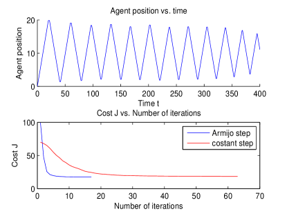
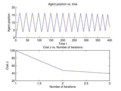
Refer to caption
(a) a=0,b=20formulae-sequence𝑎0𝑏20a=0,b=20. Ai=0.1,i=1,,20formulae-sequencesubscript𝐴𝑖0.1𝑖120A_{i}=0.1,i=1,\ldots,20. J=17.77.superscript𝐽17.77J^{\ast}=17.77.
Refer to caption
(b) a=4,b=16formulae-sequence𝑎4𝑏16a=4,b=16. Ai=0.1,i=1,,20formulae-sequencesubscript𝐴𝑖0.1𝑖120A_{i}=0.1,i=1,\ldots,20. J=39.14.superscript𝐽39.14J^{\ast}=39.14.
Refer to caption
(c) a=0,b=20formulae-sequence𝑎0𝑏20a=0,b=20. A0=A20=0.5,Ai=0.1,i=1,,19.formulae-sequencesubscript𝐴0subscript𝐴200.5formulae-sequencesubscript𝐴𝑖0.1𝑖119A_{0}=A_{20}=0.5,A_{i}=0.1,i=1,\ldots,19. J=39.30.superscript𝐽39.30J^{\ast}=39.30.
Refer to caption
(d) a=0,b=20formulae-sequence𝑎0𝑏20a=0,b=20. Ai(Δti)U(0.075,0.125)subscript𝐴𝑖Δsubscript𝑡𝑖𝑈0.0750.125A_{i}\left(\Delta t_{i}\right)\backsim U\left(0.075,0.125\right), Δti0.1e0.1tΔsubscript𝑡𝑖0.1superscript𝑒0.1𝑡\Delta t_{i}\backsim 0.1e^{-0.1t}. J=17.54.superscript𝐽17.54J^{\ast}=17.54.
Figure 3: One agent example. L=20,T=400formulae-sequence𝐿20𝑇400L=20,T=400. For each example, top plot: optimal trajectory; bottom plot: J versus iterations.
Refer to caption
(a) a=0,b=20formulae-sequence𝑎0𝑏20a=0,b=20.
Refer to caption
(b) a=4,b=16formulae-sequence𝑎4𝑏16a=4,b=16.
Figure 4: Magnified trajectory for sub-figure (a) and (b) in Fig. 3, t[0,75]𝑡075t\in\left[0,75\right].
Refer to caption
(a) a=0,b=20formulae-sequence𝑎0𝑏20a=0,b=20.
Refer to caption
(b) a=4,b=16formulae-sequence𝑎4𝑏16a=4,b=16.
Figure 5: Max, min and mean uncertainty value for each sampling point.
Refer to caption
(a) a=0,b=20formulae-sequence𝑎0𝑏20a=0,b=20. J=17.77.superscript𝐽17.77J^{\ast}=17.77.
Refer to caption
(b) a=4,b=16formulae-sequence𝑎4𝑏16a=4,b=16. J=39.14.superscript𝐽39.14J^{\ast}=39.14.
Figure 6: Two agent example. L=40,T=400formulae-sequence𝐿40𝑇400L=40,T=400. Top plot: optimal trajectory. Bottom plot: J versus iterations.

5 Conclusion

References

  • [1] I. Rekleitis, V. Lee-Shue, A. New, and H. Choset, “Limited communication, multi-robot team based coverage,” in Robotics and Automation, 2004. Proceedings. ICRA’04. 2004 IEEE International Conference on, vol. 4.   IEEE, 2004, pp. 3462–3468.
  • [2] J. Cortes, S. Martinez, T. Karatas, and F. Bullo, “Coverage control for mobile sensing networks,” Robotics and Automation, IEEE Transactions on, vol. 20, no. 2, pp. 243–255, 2004.
  • [3] W. Li and C. Cassandras, “A cooperative receding horizon controller for multivehicle uncertain environments,” IEEE Transactions on Automatic Control, vol. 51, no. 2, pp. 242–257, 2006.
  • [4] A. Girard, A. Howell, and J. Hedrick, “Border patrol and surveillance missions using multiple unmanned air vehicles,” in 43rd IEEE Conference on Decision and Control, vol. 1.   IEEE, 2005, pp. 620–625.
  • [5] B. Grocholsky, J. Keller, V. Kumar, and G. Pappas, “Cooperative air and ground surveillance,” IEEE Robotics & Automation Magazine, vol. 13, no. 3, pp. 16–25, 2006.
  • [6] S. Smith, M. Schwager, and D. Rus, “Persistent robotic tasks: Monitoring and sweeping in changing enviroments,” IEEE Transactions on Robotics, 2012, to appear.
  • [7] D. Paley, F. Zhang, and N. Leonard, “Cooperative control for ocean sampling: The glider coordinated control system,” IEEE Transactions on Control Systems Technology, vol. 16, no. 4, pp. 735–744, 2008.
  • [8] D. Bertsimas and G. Van Ryzin, “Stochastic and dynamic vehicle routing in the Euclidean plane with multiple capacitated vehicles,” Operations Research, pp. 60–76, 1993.
  • [9] R. Cooper, Introduction to queuing theory.   Edward Arnold, 1981.
  • [10] G. Sun, C. Cassandras, Y. Wardi, C. Panayiotou, and G. Riley, “Perturbation analysis and optimization of stochastic flow networks,” Automatic Control, IEEE Transactions on, vol. 49, no. 12, pp. 2143–2159, 2004.
  • [11] N. Nigam and I. Kroo, “Persistent surveillance using multiple unmanned air vehicles,” in IEEE Aerospace Conference.   IEEE, 2008, pp. 1–14.
  • [12] P. Hokayem, D. Stipanovic, and M. Spong, “On persistent coverage control,” in Decision and Control, 2007 46th IEEE Conference on.   IEEE, 2008, pp. 6130–6135.
  • [13] Y. Elmaliach, A. Shiloni, and G. Kaminka, “A realistic model of frequency-based multi-robot polyline patrolling,” in Proceedings of the 7th international joint conference on Autonomous agents and multiagent systems-Volume 1.   International Foundation for Autonomous Agents and Multiagent Systems, 2008, pp. 63–70.
  • [14] Y. Elmaliach, N. Agmon, and G. Kaminka, “Multi-robot area patrol under frequency constraints,” in Robotics and Automation, 2007 IEEE International Conference on.   IEEE, 2007, pp. 385–390.
  • [15] C. Cassandras, Y. Wardi, C. Panayiotou, and C. Yao, “Perturbation analysis and optimization of stochastic hybrid systems,” European Journal of Control, vol. 16, no. 6, pp. 642–664, 2010.
  • [16] Y. Wardi, R. Adams, and B. Melamed, “A unified approach to infinitesimal perturbation analysis in stochastic flow models: the single-stage case,” IEEE Trans. on Automatic Control, vol. 55, no. 1, pp. 89–103, 2009.
  • [17] A. Bryson and Y. Ho, Applied optimal control.   Wiley New York, 1975.
  • [18] M. Egerstedt, Y. Wardi, and H. Axelsson, “Transition-time optimization for switched-mode dynamical systems,” Automatic Control, IEEE Transactions on, vol. 51, no. 1, pp. 110–115, 2006.
  • [19] M. Shaikh and P. Caines, “On the hybrid optimal control problem: Theory and algorithms,” IEEE Transactions on Automatic Control, vol. 52, no. 9, pp. 1587–1603, 2007.
  • [20] X. Xu and P. Antsaklis, “Optimal control of switched systems based on parameterization of the switching instants,” Automatic Control, IEEE Transactions on, vol. 49, no. 1, pp. 2–16, 2004.
  • [21] C. Yao and C. Cassandras, “Perturbation analysis of stochastic hybrid systems and applications to resource contention games,” Frontiers of Electrical and Electronic Engineeing in China, vol. 6,3, pp. 453–467, 2011.
  • [22] C. Cassandras, J. Lygeros, and C. Press, Stochastic hybrid systems.   CRC/Taylor & Francis, 2007.
  • [23] E. Polak, Optimization: algorithms and consistent approximations.   Springer Verlag, 1997.