The clustering of galaxies at in the SDSS-III Data Release 9 BOSS-CMASS sample: a test for the CDM cosmology
Abstract
We present results on the clustering of galaxies in the Baryon Oscillation Spectroscopic Survey (BOSS) sample of massive galaxies with redshifts which is part of the Sloan Digital Sky Survey III project. Our results cover a large range of scales from to . We compare these estimates with the expectations of the flat CDM standard cosmological model with parameters compatible with WMAP7 data. We use the MultiDark cosmological simulation, one of the largest -body runs presently available, together with a simple halo abundance matching technique, to estimate galaxy correlation functions, power spectra, abundance of subhaloes and galaxy biases. We find that the CDM model gives a reasonable description to the observed correlation functions at , which is a remarkably good agreement considering that the model, once matched to the observed abundance of BOSS galaxies, does not have any free parameters. However, we find a deviation in the correlation functions for scales and –. A more realistic abundance matching model and better statistics from upcoming observations are needed to clarify the situation. We also estimate that about of the “galaxies” in the abundance-matched sample are satellites inhabiting central haloes with mass M☉. Using the MultiDark simulation we also study the real space halo bias of the matched catalogue finding that at large scales, consistent with the one obtained using the measured BOSS projected correlation function. Furthermore, the linear large-scale bias, defined using the extrapolated linear matter power spectrum, depends on the number density of the abundance-matched sample as . Extrapolating these results to BAO scales we measure a scale-dependent damping of the acoustic signal produced by non-linear evolution that leads to – dips at level for wavenumbers in the linear large-scale bias.
keywords:
cosmology: large-scale structure of the Universe – cosmology: theory – galaxies: general – methods: observational – methods: numerical1 Introduction
The clustering of galaxies is a fundamental measure of the statistical properties of the cosmic density field through cosmic time. In the last decade, it became possible to determine the clustering strength of galaxy populations at spatial scales out to tens of Mpc and beyond with reasonable accuracy by means of massive galaxy surveys such as the Two-Degree Field Galaxy Redshift Survey (e.g., Colless et al., 2001) and Sloan Digital Sky Survey (SDSS-I/II; e.g., Gunn et al., 1998; York et al., 2000; Gunn et al., 2006). These and previous studies have shown that the correlation function is not a simple power-law and that the correlation length of luminous and massive galaxies is larger than that of less luminous ones (see Zehavi et al., 2011, and references therein).
The Baryon Oscillation Spectroscopic Survey (BOSS; e.g., Bolton et al., 2012; Smee et al., 2012; Dawson et al., 2013), a branch of the ongoing SDSS-III (Eisenstein et al., 2011), is considerably increasing the size of available galaxy samples. BOSS consists of galaxy and quasar spectroscopic surveys over a sky area of 10,000 deg2 and its main goal is to measure the BAO feature at high precision. Specifically, BOSS aims at measuring the redshifts of about 1.5 million galaxies out to . It will also acquire about 150,000 Ly forest spectra of quasars in the range , to map the large-scale distribution of galaxies at these earlier epochs (see Slosar et al., 2011). The effective volume of the galaxy survey is expected to be about 7 times higher than that of the SDSS-I/II Luminous Red Galaxy (LRG) sample which consisted of LRGs out to . The selection criteria of the BOSS targets result in a sample of massive, and hence highly clustered systems, which are suitable candidates for a reliable detection of the Baryon Acoustic Oscillation (BAO) clustering signal that can be used to constrain the expansion history of the Universe (e.g., Anderson et al., 2012; Reid et al., 2012; Sánchez et al., 2012). Additionally, the project also provides a wealth of other information on clustering and physical properties of galaxies.
Requirements for theoretical predictions of galaxy clustering in BOSS are extreme: one needs accurate predictions for very large volumes in order to compare with observations. Therefore, the combination of large-volume cosmological -body simulations with prescriptions to associate galaxies with dark matter haloes turns out to be the most efficient way to generate the required model galaxy samples. Recently, White et al. (2011) presented clustering results for scales in the range – based on galaxies in the redshift range obtained during the first semester of BOSS operation. To compare these observational results with theory, the authors combined large, albeit low-resolution, -body simulations with the Halo Occupation Distribution (HOD) model (e.g., Berlind & Weinberg, 2002; Kravtsov et al., 2004; Zentner et al., 2005; Skibba & Sheth, 2009; Ross & Brunner, 2009; Ross et al., 2010). Their results suggest that the majority of BOSS galaxies are central systems living in haloes with a mass of M☉, while about 10% of them are satellites typically residing in haloes times more massive.
The HOD approach is the most often used framework to make predictions for the large-scale distribution of galaxies. Alternatively, HODs can also be measured in observations (Zehavi et al., 2005; Abazajian et al., 2005; Brown et al., 2008; Zheng et al., 2009). The main component of classical HOD models is the probability, , that a halo of virial mass hosts galaxies with some specified properties. In general, theoretical HODs require the fitting of a function with several parameters (e.g., Kravtsov et al., 2004; Zheng et al., 2005), which gives some freedom to match the observed clustering of galaxies. These models also depend on the theoretical approach adopted to predict the galaxy number inside haloes of mass . For example, Zheng et al. (2005) used SPH simulations and semi-analytical models to measure the number of galaxies as a function of hosting halo mass, which is definitely a challenging theoretical exercise. White et al. (2011) tuned five HOD free parameters to fit the observed clustering of galaxies. In this case a random fraction of dark matter particles is selected from the simulations with a fraction following the optimized HOD. This prescription will have the best match to observations hence producing good-quality mock catalogues. However, different choices of the underlying cosmology might lead to different HOD parameters. Kravtsov et al. (2004) use a different approach: they identify subhaloes in high-resolution -body simulations in order to associate them with satellite galaxies. This is an attractive path, which can be further perfected by more accurate simulations and more elaborate prescriptions for “galaxies” in dark matter-only simulations (e.g., Trujillo-Gomez et al., 2011).
Halo Abundance Matching (HAM) has recently emerged as an alternative to HOD in order to bridge the gap between dark matter haloes and galaxies (Kravtsov et al., 2004; Tasitsiomi et al., 2004; Vale & Ostriker, 2004; Conroy et al., 2006; Kim et al., 2008; Guo et al., 2010; Wetzel & White, 2010; Trujillo-Gomez et al., 2011; Reddick et al., 2012). Abundance-matching resolves the issue of connecting observed galaxies to simulated dark matter haloes and subhaloes by setting a one-to-one correspondence between the red-band luminosity or stellar and dynamical masses: more luminous galaxies are assigned to more massive (sub)haloes (in what follows we will write “(sub)haloes” to account for all haloes and subhaloes). By construction, the method reproduces the observed luminosity function (or stellar mass function). It also reproduces the scale dependence of galaxy clustering over a large range of epochs (Conroy et al., 2006; Guo et al., 2010). When abundance matching is used for the observed stellar mass function (Li & White, 2009), it gives also a reasonable fit to lensing results (Mandelbaum et al., 2006) and to the relation between stellar and virial mass (Guo et al., 2010). Guo et al. (2010) also attempted to reproduce the observed relation between the stellar mass and the maximum circular velocity with partial success finding deviations both in shape and amplitude between model and observations. For instance, at circular velocities in the range – km s-1 the estimated circular velocity was % lower than the observed one. They proposed that this disagreement is likely due to the fact that they did not include the effect of baryons. Indeed, Trujillo-Gomez et al. (2011) show that accounting for baryons drastically improves the situation.
Just like as with HODs, there are different flavours of HAMs. Generally, one does not expect a pure monotonic relation between stellar and dynamical masses. There should be some degree of stochasticity in this relation due to deviations in the merger history, angular momentum, and halo concentration. Even for haloes (or subhaloes) with the same mass, these properties should be different for different systems, which would lead to deviations in stellar mass. Observational errors are also responsible in part for the non-monotonic relation between halo and stellar masses. Most of modern HAM models already implement prescriptions to account for the stochasticity (Tasitsiomi et al., 2004; Behroozi et al., 2010; Trujillo-Gomez et al., 2011; Leauthaud et al., 2011). The difference between monotonic and stochastic models depends on the magnitude of the scatter and on the stellar mass. The typical value of the scatter in the -band is expected to be – mag (e.g., Trujillo-Gomez et al., 2011). For the Milky-Way-size galaxies the differences are practically negligible (Behroozi et al., 2010), but they increase for very massive galaxies such as those targeted with BOSS due to the strong dependence of the bias with mass.

Almost two years after the start of the project, BOSS has obtained the spectra of about 536,000 galaxies and 102,000 quasars (Ahn et al., 2012). Using the SDSS-III Data Release 9 (DR9) BOSS data we present results on the two-dimensional, projected and redshift-space correlation functions on scales from to including fibre collision corrections. In order to account for the CDM cosmological model we use a large high-resolution -body simulation with a resolution high enough to resolve subhaloes, which is very important for the HAM prescription. When connecting haloes with galaxies we use a stochastic HAM model.
This paper is organized as follows. In Section 2 we present the BOSS galaxy sample studied here, dubbed “CMASS”, and the measurements of the two-dimensional, projected and redshift-space galaxy clustering in observations. In Section 3 we present the details of the MultiDark simulation, the halo catalogues and the HAM technique adopted here. In Sections 4 and 5 we compare the clustering measures with observations and study the occupation distribution given by our halo catalogue. We also discuss the comparison between our halo occupation distribution with that obtained by White et al. (2011) using an HOD model. In Section 6 we study the scale-dependent bias of galaxy clustering of the CMASS sample as inferred from our HAM model and MultiDark simulation both in real and Fourier space. Finally, in Section 7 we close the paper with the summary and conclusions. Throughout this paper we assume MultiDark cosmological parameters (see Section 3.1).
2 Observations
2.1 The CMASS sample
In this section we introduce the BOSS sample of massive galaxies analyzed in this work. The target galaxies are selected in such a way that the stellar mass of the systems is approximately constant over the entire redshift range of interest. As a consequence, the resulting galaxy sample is usually dubbed ‘constant mass’ (CMASS) sample. These galaxies are characterized by high-luminosities which translate in a rather low comoving space density of about . The sample can be obtained by applying the following colour cuts to the observations (see e.g. Eisenstein et al., 2011; Anderson et al., 2012):
| (1) |
where and is the magnitude measured with the 2′′ BOSS fiber within the SDSS photometric system (Fukugita et al., 1996). The subscripts cmod and mod denote “cmodel” and “model” magnitudes respectively. These cuts are chosen to pick out massive red galaxies at . In particular, the condition selects systems with observed red colours, whereas the conditions imposed on the -magnitude is designed to identify an approximately complete galaxy sample down to a limiting stellar mass. Most of these galaxies () show an early-type morphology with a characteristic stellar mass of M☉ and an absolute -band magnitude of (Masters et al., 2011).
Schlafly et al. (2010) and Schlafly & Finkbeiner (2011) found systematic offsets between the colours of SDSS objects in the southern and northern Galactic hemispheres which might reflect a combination of percent calibration errors in the SDSS photometry and errors in the corrections for Galactic extinction. The Schlafly & Finkbeiner (2011) results suggest a systematic offset in the value of of 0.0064 between the north and south. As the CMASS selection criteria depends on , this offset leads, in principle, to a difference in the galaxy samples selected for spectroscopic observations in the two hemispheres. Ross et al. (2011) found a 2% difference in the number density of CMASS targets between the northern and southern hemispheres, which reduces to 0.3% when this offset is applied to the galaxies in the south before applying the CMASS selection criteria. However, Ho et al. (2012) found no appreciable north/south colour offsets in their sample. In this work we do not apply a colour offset to the selection of CMASS galaxies in the south. Although we present results obtained from the combined (northsouth) CMASS sample, we also analyse the data from the northern and southern hemispheres separately in order to avoid potential systematics that could be associated with the use of slightly different selection criteria.
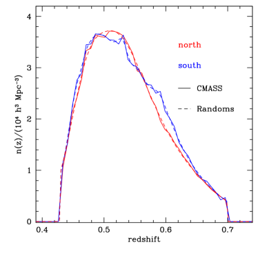
For a number of reasons it is not possible to obtain reliable redshifts for all the galaxies satisfying the CMASS selection criteria (see Section 2.2). We estimate the completeness , where is the number of galaxy targets and the number of these with reliable redshift estimates (weighted as described in Section 2.2) for each sector of the survey mask, that is, the areas of the sky covered by a unique set of spectroscopic tiles (Blanton et al., 2003; Tegmark et al., 2004) which we characterize using the Mangle software (Hamilton & Tegmark, 2004; Swanson et al., 2008). The average completeness of the combined CMASS sample is 98.2%. We trim the final area of our sample to all sectors with completeness , producing our final sample of 282,068 galaxies, of which 219,773 and 62,295 are located in the northern and southern galactic caps respectively. Fig. 1 shows an Aitoff projection of the resulting survey mask in the northern (upper panel) and southern (lower panel) regions, with effective areas , where the sum extends over all sectors contained in the mask and corresponds to their solid angles, 2502 deg2 and 688 deg2 respectively. The redshift distribution of the CMASS sample can be seen in Fig. 2 both for the north and south subsamples. The dashed lines show the smoothed distributions used to create the random samples of points for our clustering analysis (see Section 2.2). As shown in this figure the galaxy number density peaks at having a value of and a mean redshift of .
2.2 Clustering measures
We characterize the clustering of the CMASS galaxy sample by means of two-point statistics in configuration space. We measure the angle-averaged redshift-space correlation function and the full two-dimensional , where and are the components in the direction perpendicular and parallel to the line of sight of the total separation vector . These measurements are affected by redshift-space distortions. In order to obtain a clustering measure that is less sensitive to these effects we also compute the projected correlation function (Davis & Peebles, 1983)
| (2) |
In practice, we sum all pairs with using linearly-spaced bins. We have checked that the projected correlation has already converged for .
We compute the full correlation functions using the Landy & Szalay (1993) estimator
| (3) |
where , , and are the suitably normalized numbers of data-data, data-random, and random-random pair counts in each bin of . In order to measure these quantities without introducing systematic effects, a few important corrections must be taken into account. Here we give a brief description of the main issues that should be considered while a more detailed discussion will be presented in Ross et al. (2012).
As described in the previous section, the spectroscopic CMASS sample is constructed from a target list drawn from the SDSS photometric observations. Even though the overall completeness of the CMASS sample is high, it is not possible to obtain reliable redshifts for all galaxies satisfying the selection criteria specified in Section 2.1. Which galaxies are observed spectroscopically is determined by an adaptive tiling algorithm, based on that of Blanton et al. (2003), which attempts to maximize the number of measured spectra over the survey area. As a result of this algorithm, not all galaxies satisfying the CMASS criteria are selected as targets for spectroscopy. Even when a fibre is assigned to a galaxy and a spectrum is observed, it might not be possible to obtain a reliable estimation of the redshift of the object, leading to what is called a redshift failure. These tend to occur for fibres located near the edges of the observed plates. This implies that it is not possible to simply consider these redshift failures as an extra component affecting the overall completeness of the sector since their probability is not uniform across the field. In order to correct for this effect we define a set of weights, , whose default value is one for all galaxies in the sample. For every galaxy with a redshift failure, we increase by one the value of of the nearest galaxy with a good redshift measurement. The application of these weights effectively corrects for the non-uniformity effects produced by redshift failures.
The main cause for the loss of objects is, however, fibre collisions (Zehavi et al., 2002; Masjedi et al., 2006). The BOSS spectrographs are fed by optical fibres plugged on plates, which must be separated by at least (in the concordance cosmology this corresponds to a distance of at ). It is then impossible, in any given observation, to obtain spectra of all galaxies with neighbours closer than this angular distance. The problem is alleviated in regions covered by multiple exposures, but it is in general not possible to observe all objects in crowded regions.
In this work we correct for the impact of fibre collisions on our clustering measurements by applying the correction presented in Guo et al. (2012). Using this method the total galaxy sample is divided into two subsamples, dubbed as and . These are constructed following the targeting algorithm of the catalogue in a way that guarantees that group is not affected by fibre collisions, while contains all collided galaxies. Any clustering measurement of the combined sample can be obtained as a combination of the contributions from these two groups. Based on tests on mock galaxy catalogues, Guo et al. (2012) showed that the application of this method can accurately recover the projected and redshift-space correlation functions on scales both below and above the fibre collision scale, providing a substantial improvement over the commonly used nearest neighbour and angular correction methods.
We constructed random catalogues for subsamples and for the northern and southern hemispheres with 40 times more objects than the real data following their respective angular completenesses. The redshifts of these random points were generated in order to follow the distributions of the real samples, which were obtained by a smoothing spline interpolation of the observed redshift distributions (see dashed lines in Fig 2).
With the increasing size of current galaxy surveys, and the corresponding improvement on the statistical uncertainties, the contribution of systematic errors to the total error budget of any clustering statistic becomes increasingly important. Due to its large volume and high number density BOSS is perhaps one of the best examples of this. Ross et al. (2012) present a detailed analysis of the systematic effects that could potentially affect any clustering measurement based on the CMASS sample and show that, besides redshift failures and fibre collisions, other important systematics must be considered in order to obtain accurate clustering measurements. The main result from this analysis is that these systematics can be corrected for by applying a set of weights, , which depend on both, the galaxy properties and their positions in the sky. We consider these weights in all our clustering measurements.
Finally, we also include a set of weights to reduce the variance of the estimator that are given by
| (4) |
where is the mean galaxy density at redshift and is a free parameter. Hamilton (1993) showed that setting , where , minimizes the variance on the measured correlation function for the given scale . Here we follow the standard practice and use a scale-independent value of .
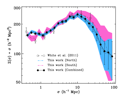
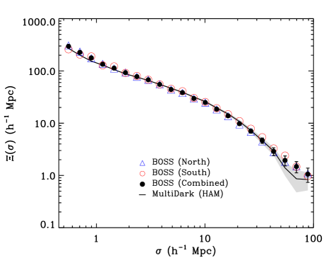
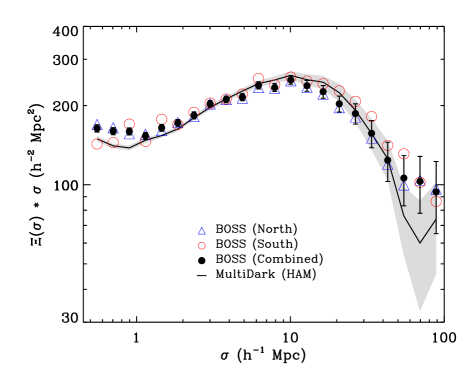
Fig. 3 shows the projected correlation functions times the projected distance of the north, south and combined CMASS samples. The combined sample gives a similar outcome to that of the north as a result of the higher statistics in the latter. For comparison the projected correlation inferred from a CMASS sample corresponding to the first semester of the BOSS observations is also shown (open circles; White et al., 2011). Besides the increase in the sample size and the volume probed, there are differences at small and large scales which are probably due to the different corrections for fibre collisions and the use of the weights to correct for the systematics affecting the galaxy density field.
Although the projected correlation functions of the north and south subsamples agree within their respective uncertainties, they show some intriguing differences. At scales in the range – the amplitude of in the south is higher than that of the north. Similarly, the measurements of show the same behaviour. However, in this case, the agreement of the mean values is somewhat closer. In Section 4 we present further results on these clustering measures for the north, south and combined BOSS-CMASS galaxy samples separately.
2.2.1 Estimation of covariances in the data
To estimate covariance matrices for these clustering measures, we use a set of 600 mock catalogues designed to follow the same geometry and redshift distribution of the CMASS sample while mimicking their clustering properties at large scales (Manera et al., 2013). These mocks are inspired by the PTHalos method of Scoccimarro & Sheth (2002) which is aimed at computing the evolution of structure using Lagrangian perturbation theory including several prescriptions to account for haloes at smaller scales. However, we note that some important differences exist between both treatments. The resulting covariances are compatible with the results of -body simulations (see Section 3.3.1) while displaying convergence at a few percent-level for the range of scales studied here. For a detailed description about these mocks and their comparison with -body results see Manera et al. (2013)111Mocks will be available in http://www.marcmanera.net/mocks/. In Appendix B we provide tables for the estimated correlation matrices of the projected and redshift-space correlation functions for the north, south and combined BOSS-CMASS samples.
3 Clustering in the CDM model
3.1 The MultiDark simulation
The MultiDark run (MDR1) is an -body cosmological simulation of the CDM model that was done using the Adaptive-Refinement-Tree (ART) code (Kravtsov et al., 1997; Gottlöber & Klypin, 2008). The simulation has 2048 dark matter particles in a box of 1 Gpc on a side. The mass of the dark matter particle is M☉. The cosmological parameters adopted in the simulation are consistent with the latest WMAP7 results (Jarosik et al., 2011) and with other cosmological probes (see Table 1 of Klypin et al., 2011). Hence, we adopt a matter density parameter and a dimensionless Hubble parameter . Initial conditions were set at the redshift using a power spectrum characterized by a scalar spectral index and normalized to in the same way as done for the Bolshoi simulation (see Klypin et al., 2011, for a detailed description of this simulation). Since the adopted cosmological parameters are very close to the latest observational estimations any departure from the true cosmology will not affect our main results. The ART code is designed in such a way that the physical resolution is nearly preserved over time with a value of kpc for the redshift range between –. For further details on the ART code and MultiDark simulation see Prada et al. (2012) and references therein.
3.1.1 Halo finding
Dark matter haloes are identified in the simulation with a parallel version of the Bound-Density-Maxima (BDM) algorithm (Klypin & Holtzman, 1997; Riebe et al., 2011). The BDM is a Spherical Overdensity (SO) code. It finds all density maxima in the distribution of particles using a top-hat filter with 20 particles. For each maximum the code estimates the radius within which the overdensity has a specified value. Among all overlapping density maxima the code finds the one having the deepest gravitational potential. The position of this maximum is the centre of a “distinct” halo, which is a halo whose centre is not inside the virial radius of a bigger one. Distinct haloes are also tracers of central galaxies. Self-bound haloes with more than 20 particles lying inside the virial radius of a distinct halo are classified as subhaloes. Subhalo identification is more subtle since it requires the removal of unbound particles and identification of fake satellites (see Riebe et al., 2011, for a detailed description of this method). The BDM algorithm was extensively tested and compared with other halo finders (Knebe et al., 2011; Behroozi et al., 2013). In Appendix A.1 we show a comparison between the real-space correlation function for halo catalogues selected both with BDM and RockStar halo finders (see Fig 15). The BDM halo catalogues for the MDR1 simulation are publicly available at the MultiDark Database: http://www.multidark.org.
The size of a distinct halo can be defined by means of the spherical radius within which the average density is times higher than the critical density of the Universe, . As a consequence, the corresponding enclosed mass is given by
| (5) |
We use a threshold overdensity of that results in values for halo mass and radius of and respectively. In addition, BDM catalogues also provide virial masses and radius ( and ) defined using the standard overdensity , where is the background mean density of the Universe.
One of the most important characteristics of a (sub)halo is its maximum circular velocity at redshift :
| (6) |
There are several advantages of using at a given time to characterize the dynamical mass of a halo as opposed to the “virial mass”. First, does not have the ambiguity related with the definition of mass. Virial mass and radius vary depending on the overdensity threshold used. For the oftenly employed overdensity 200 and “virial” overdensity thresholds, the differences in definitions result in changes in the halo radius from one definition to another and, thus, in concentration, by a factor of –, where the exact value depends on the halo concentration. Second, and more important, the maximum circular velocity is a better quantity to characterize haloes whenever is needed to relate them to their associated galaxies. For instance, for galaxy-size haloes the maximum circular velocity is defined at a typical radius of kpc, i.e., much closer to the sizes of luminous parts of galaxies than the virial radius, which for the Milky-Way halo is of the order of (Klypin et al., 2002).
3.2 Bridging the gap between galaxies and haloes
To select a simulated halo sample representing BOSS-CMASS galaxies we apply the HAM technique. Once we have the maximum circular velocities for distinct haloes and subhaloes the implementation of the HAM prescription is simple: we start with a monotonic assignment. We count all haloes and subhaloes, which have maximum circular velocity larger than the threshold , and gradually decrease the value of until the number density of (sub)haloes is equal to that of BOSS galaxies at .
A usual choice for is to take the halo maximum circular velocity at as a measure of the dynamical mass of the system since this is a quantity that can be easily obtained from simulations. However, it is generally accepted that, for subhaloes, a better characteristic would be the peak value of the maximum circular velocity, , during the entire subhalo evolution (e.g., Conroy et al., 2006; Trujillo-Gomez et al., 2011). The latter is related to the tidal stripping effect: once a halo falls into the potential well of a larger one some of its material can be stripped away, thus lowering the value of . Since in real galaxies stars occupy the inner regions of subhaloes, where tidal forces are much weaker, their circular velocities should be, in general, less influenced by this effect. For instance, Watson et al. (2012), based on a subhalo evolution model applied to clustering measurements in the SDSS, suggest that tidal stripping of stars in luminous galaxies (as those presumably expected in the BOSS-CMASS sample) is much less efficient than in less luminous systems. Nevertheless, when it comes to matching (sub)haloes to the galaxy abundance one should use the best theoretically motivated parameter, which in this case is . Hence, in what follows, we will adopt this quantity as a measure of the dynamical mass of (sub)haloes in the simulation.
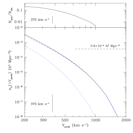
The bottom panel of Fig. 4 shows the number density of (sub)haloes at in the MultiDark simulation as a function of . A number density close to that of the BOSS-CMASS sample corresponds to (sub)haloes with a peak maximum circular velocity above 370 km s-1, which is sufficiently larger than the completeness limit of the MultiDark simulation, i.e., . This means that (sub)haloes hosting BOSS-CMASS galaxies are well resolved. The top panel of Fig. 4 shows the cumulative subhalo fraction as a function of maximum circular velocity. For values of the subhalo fractions are typically less than . We will return to this point again in Section 5.
3.2.1 Halo stochasticity
There are a number of arguments why there should be some degree of stochasticity in the stellar mass – circular velocity relation (e.g., Tasitsiomi et al., 2004; Behroozi et al., 2010; Trujillo-Gomez et al., 2011). In our case the stochasticity means that some haloes above the velocity cut host galaxies with stellar masses smaller than the corresponding stellar mass cut of the BOSS sample and should not be included into the sample. Simultaneously, some smaller haloes may host galaxies with a larger stellar mass, and should be considered. Because the number density of galaxies is fixed by observations, the numbers of included and excluded haloes must be equal. Following Trujillo-Gomez et al. (2011) we implement this process using a Gaussian spread with an offset. If is the velocity cut in the monotonic assignment, then a (sub)halo is taken if its peak maximum circular velocity satisfies the condition
| (7) |
where is a Gaussian random number with mean zero and rms . The offset is needed to compensate the larger influx of smaller haloes. We use and , which are consistent with the values adopted by Trujillo-Gomez et al. (2011). Note that the offset and the spread are not free parameters. The offset is just a normalization. The value of is defined by the spread of the observational Baryonic Tully-Fisher relation (or its equivalent for early-type galaxies), which has uncertainties (e.g., Trujillo-Gomez et al., 2011). The stochastic assignment has a very small effect on clustering for scales larger than decreasing the correlation functions no more than .
3.3 Modelling BOSS-CMASS clustering
We use the MultiDark BDM catalogues constructed for the overdensity to facilitate the comparison with the HOD modelling presented in White et al. (2011). However, as stated before, our results do not depend on halo mass definition since halo matching is done using the peak maximum circular velocity of either distinct haloes or subhaloes. For the HAM to the BOSS-CMASS sample we choose a redshift of and an effective number density of (see Fig. 2). However, our clustering results are mostly insensitive to small deviations around these fiducial values as it is shown in appendices A.2 and A.3 respectively.
To model the effect of galaxy peculiar velocities in the redshift measurements, we transform the coordinates of our simulated (sub)haloes to redshift-space using + , where and are their position and peculiar velocity vectors respectively, is the scale factor and is the Hubble constant. We compute the two-dimensional correlation function of our catalogue counting the number of “galaxy” tracers in bins parallel () and perpendicular () to the line-of-sight. When estimating the projected correlation function, we count all pairs along the parallel direction out to using linearly-spaced bins. We have checked that our model projected correlation function has already converged for .
3.3.1 Estimation of cosmic variance in MultiDark
Our estimation of the (sub)halo clustering corresponding to the BOSS number density in a CDM cosmology is limited by the finite volume of the MultiDark simulation. To estimate the expected level of cosmic variance we use a set of low-resolution simulations from the Large Suite of Dark Matter Simulations (LasDamas; see http://lss.phy.vanderbilt.edu/lasdamas/). In particular, we use the Carmen boxes, which are 40 dark matter-only runs done with particles in a periodic cube with Gpc on a side. The dark matter density and scalar spectral index of the Carmen simulations display a difference of about in comparison to the corresponding values of MultiDark. However, since here we only want to obtain an estimate for the magnitude of the cosmic variance, we consider this approach as good enough for our purpose.
For all Carmen runs we used halo catalogues matched to the abundance of the BOSS-CMASS sample at as explained in Section 3.2. This allowed us to get the magnitude of cosmic variance in the clustering signal. In this way, we can get a simple estimate of the expected rms deviations of our MultiDark results due to random fluctuations in the intial conditions of the universe.
As mentioned in Section 2.2.1, the estimation of cosmic variance in the observed correlation functions is done using the covariance matrices of a set of 600 galaxy mocks designed to follow the same geometry and redshift distribution of the CMASS sample, while mimicking its clustering properties at large scales. Manera et al. (2013) show that the covariances for the correlation functions of -body simulations are consistent with those resulting from the mocks. However, it is important to keep in mind that the clustering measures of the mocks are not a good representation of the clustering in the BOSS-CMASS sample at the smallest scales. This is due to the fact that the mocks are constructed using Lagrangian perturbation theory including approximations which break down at small scales. However, we checked that the magnitude of the variance obtained both from the PTHalos mock catalogues and LasDamas set of -body simulations displays good consistency, after rescaling them to take into account for the difference in their effective volumes. We conclude then that it is safe to compare the cosmic variance of MultiDark (estimated from the Carmen set of simulations) with that resulting from the mock galaxy catalogues. In Section 4 we present the MultiDark HAM clustering results in comparison with our observational clustering estimates.
4 Clustering of galaxies in the BOSS-CMASS sample: results from model and observations
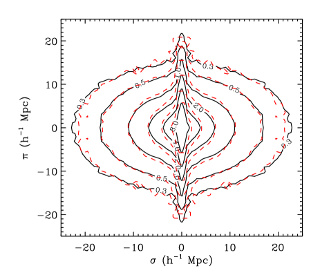
The two-dimensional correlation function for the north subsample of BOSS-CMASS is presented in Fig. 5 for distances up to (dashed contours). The Finger-Of-God elongation along the line-of-sight direction at small perpendicular separations, which is due to galaxy small-scale random velocities, is clearly seen. The flattening of contours at larger projected scales is due to the Kaiser effect caused by large-scale infall velocities (Kaiser, 1987). The clustering of “galaxies” obtained with the MultiDark cosmological simulation (solid contours) produce a fair representation of the measured clustering in the CMASS sample. Nevertheless, there are some deviations. At small separations, , observations show more clustering as compared with results from the simulation. The situation reverses at large scales (), where our cosmological simulation results in a slightly stronger clustering.
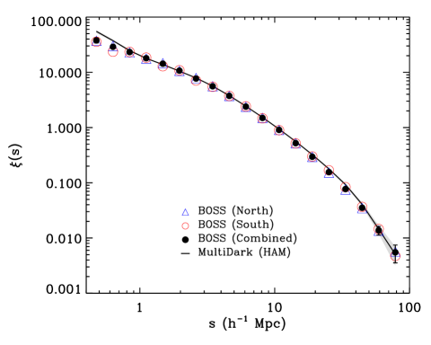
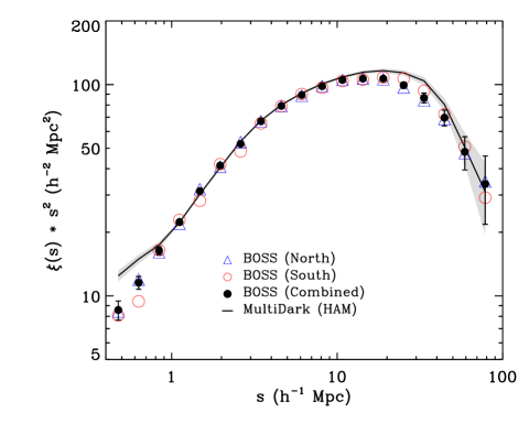
The projected and redshift-space correlation functions for the observed and halo samples considered in this work are presented in Figs. 6 and 7. The north, south and combined CMASS samples (symbols) are shown together with the result of our simple HAM model (solid lines). The shaded area for MultiDark gives an estimate of the cosmic variance as computed from LasDamas suite of simulations.
As noted before, there are some noticeable discrepancies at small and intermediate scales. The detailed differences between the projected correlation function and MultiDark can be better seen in the right panel of Fig. 6, where differences in the correlations are amplified after multiplying by the corresponding projected distance. The disagreement at scales is of the order of . At larger scales (–) the theoretical estimates lie slightly above those of the north galaxy subsample (which has about four times larger statistics than the corresponding southern sample) but they are still consistent with each other within level.
The redshift-space clustering results, both for the CMASS sample and the CDM model given by the MultiDark simulation, are shown in Fig. 7. As before, the shaded area represents cosmic variance estimates and differences between model and observations are better seen in the right panel. Peculiar velocities of galaxies inside virialized systems reduce the clustering signal thus lowering the slope of the correlation function at scales of –.
For scales in the range – our simple HAM overpredicts the observed values by an amount of the order of . At larger scales () the matching between the model and observations improves significantly. Differences are less than for a wide range of distances ranging from to about . At – the MultiDark result overpredicts the observed clustering by . Statistically, the differences are significant: the effect is about at (e.g., at the redshift-space correlation function for the combined CMASS sample and MultiDark gives and , respectively). At scales our HAM model and observations are consistent within . In tables 2 and 3 (see Appendix B) we present measurements and standard deviations of the correlations shown in Figs. 6 and 7.
Despite of differences the overall match is quite good considering the simplicity of our method: the only free parameter used in our HAM is the abundance of (sub)haloes present in the simulation. The disagreement between the -body results and observations could be related to the simple stochastic HAM adopted here and may be alleviated using a more sophisticated procedure including, for instance, light-cone effects and a match to the stellar mass distribution of the sample at these redshifts. On the other hand, the mismatch could also be due to some difference between the true cosmology and the one adopted for our simulation. In the following sections we will exploit the information encoded in our BOSS-CMASS abundance-matched halo sample as a way to shed some light on the actual trends of the real galaxy population.
5 The mean halo occupancy of the abundance-matched halo sample
After fixing the abundance of (sub)haloes to that given by observations the simulated subhalo distribution is completely determined by the cosmological model adopted and the resolution of the simulation. The main advantage of the MultiDark simulation is that it has sufficient resolution to resolve massive satellites around our central distinct haloes. Therefore, the satellite distribution around haloes can be directly studied from the matched halo catalogues. As shown previously in the top panel of Fig. 4, the fraction of subhaloes around central haloes with a number density similar to that of the CMASS sample is close to . In particular, for haloes having km s-1, which corresponds to a number density of , the resulting subhalo fraction is with negligible statistical uncertainties. The HOD modelling by White et al. (2011), using the first semester of BOSS data, reported a satellite fraction which is reduced to when they ignore in their fit to the correlation function at small scales affected by fibre collisions. Note that our HAM procedure is non-parametric and provides subhalo fractions consistent with our CDM cosmological simulation. In that respect, our approach is different from HOD modelling: as mentioned in the introduction in the latter case the halo-occupancy distribution and satellite fractions are obtained from a fit to the empirical correlation function.
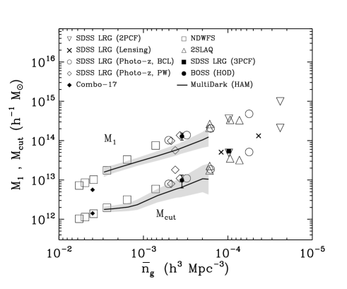
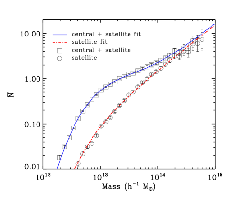
Fig. 8 shows the mean occupancy of haloes as obtained from the MultiDark halo abundance-matching scheme. The open circles represent the contribution of subhaloes while open squares correspond to the total occupancy of haloes, including both central and satellite “galaxies” from our halo catalogue. Distinct haloes display a clear transition around M☉ (see solid line). The mean number of subhaloes as a function of halo mass can be accurately described by a function of the form (e.g., Wetzel & White, 2010)
| (8) |
where , and are the best fit values (dot-dashed line). Here, is the halo mass which hosts, approximately, one satellite and governs the strength of the transition between systems with and without satellites. For high halo masses, fluctuations in the determination of the satellite occupancy arise because we are dealing with small number statistics as a result of the fixed volume of the simulation. The solid line in Fig. 8 shows the total mean halo occupancy but using in this case the best fit model for the satellite distribution in order to extrapolate the result towards higher masses.
In Fig. 9 we compare the HOD parameters, and , obtained from MultiDark at as a function of (sub)halo number density (solid lines) following our HAM scheme. This figure also shows estimates for a variety of intermediate redshift massive galaxy samples from the literature, including the HOD results from White et al. (2011) for the early BOSS data sample. This compilation of different datasets has been kindly provided by M. White. Error bars on the individual points are typically dex. The agreement between the MultiDark HAM estimations of and and those from different surveys is remarkable if one considers the differences in sample selection, redshift range and HOD methods. In particular, our estimates for the HOD parameters tend to be smaller than those of White et al.’s., which is consistent with the larger subhalo fraction found in our case. Nevertheless, both estimations marginally agree at the 1 level.
Finally, note that White et al. (2011) did not include the weights considered by Ross et al. (2012) to correct for systematic effects in the CMASS galaxy density field. In principle, this could have an impact in the estimation of their correlation functions and, as a consequence, on the derived parameters. On the other hand, it is important to keep in mind that our results rely completely on our halo catalogue.
6 Biases of the abundance-matched halo and BOSS-CMASS samples
In Section 6.1 we focus our work on the estimation of the abundance-matched halo and BOSS-CMASS galaxy biases, and their comparison, using the real-space and projected correlation functions respectively; whereas Section 6.2 focuses on the abundance-matched halo bias from power spectra.
6.1 Abundance-matched halo and galaxy biases from correlation functions
Using the resulting halo sample and dark matter particles from the simulation we can estimate the real-space bias, , of the halo population with respect to the underlying mass distribution by the following relation
| (9) |
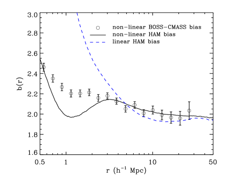
where and are the real-space correlation functions (i.e., no redshift-space distortions) for the MultiDark haloes and dark matter in the volume at the considered redshift. This is shown in Fig. 10 as a function of spatial scale (solid line). At the transition scale of the bias reaches a local minimum, increasing strongly towards smaller scales where galaxies are more strongly clustered with respect to the dark matter. The bump-like feature between – is related to the transition between the one- and two-halo terms in the correlation function, while for larger scales the bias factor tends to decrease. For scales we can constrain the abundance-matched halo bias to be in the range –, approaching for the largest radii (see also section 6.2.2).
The linear bias estimation is shown as a dashed line, where the linear matter correlation function is used instead. The latter is computed from the initial matter power spectrum of the simulation scaled to the redshift of interest according to linear theory. As expected, the linear bias at small scales differs strongly from the non-linear result while approaching more similar values at larger scales.
We also estimated the scale-dependent bias of the BOSS-CMASS sample up to (circles in Fig. 10) given by the square root ratio of the observed projected correlation function (as presented in Fig. 6; solid circles) and the non-linear projected correlation function of matter given by MultiDark at . This approach is, to first order, very close to that inferred from the real-space correlation functions by means of Eq. (9). The error bars were estimated propagating the errors adopted in observations. As shown in Fig. 10, for scales larger than the abundance-matched halo and galaxy biases display a good agreement within the error bars; whereas for smaller scales the BOSS-CMASS galaxy bias lies above that of the abundance-matched halo sample in accordance with the mismatch found between the HAM and BOSS-CMASS projected correlation functions (see Fig. 6).
Interestingly, these results are in very good agreement with the findings of Ho et al. (2012). These authors found a linear galaxy bias of in the redshift bin of – by studying the angular clustering of the photometric CMASS sample. In what follows we will extend this analysis to Fourier space to better characterize the scale-dependence of the abundance-matched halo bias.
6.2 Abundance-matched halo bias from power spectra
Here we present the clustering bias of the abundance-matched halo sample in Fourier space by means of its power spectrum since it is well known that this statistics is better suited to separate effects on different scales.
We want to present an approximation of our numerical results for the comological model adopted in the simulation since it is usually more convenient to use analytical approximations instead of dealing with raw simulations. Additionally, the derived bias dependence can motivate further comparisons with observational results. Interestingly, the high quality of our results allows us to study effects which are difficult to measure with low-resolution simulations.
One should clearly understand the role of the standard CDM model with the particular set of cosmological parameters used for our simulations. Our results show that, once we match the abundance of haloes, the model reasonably reproduces a wide range of scales of the observed projected and redshift-space correlation functions despite of some discrepancies at small and medium scales as presented in Section 4. In principle, one can invert the correlation function to obtain the power spectrum. However, in practice, a model-independent inversion is a technically complicated process. This is why we chose a different approach: we use the power spectrum of haloes in the model as an approximation of the actual power spectrum of galaxies in BOSS-CMASS for scales larger than and up to those close to BAOs.
Additionally, we use two other sets of simulations besides MultiDark. The first one is the already mentioned Carmen series of 40 simulations of the LasDamas set that allow us to estimate the effect of cosmic variance. Note that, as before, we use only relative model-to-model deviations in the Carmen simulations: error bars in our results are obtained in this way. Secondly, we also use results of the Bolshoi simulation (Klypin et al., 2011). This simulation has a factor of better mass and force resolution, but it was performed for a smaller simulation box ( on a side). There is an overlap between the MultiDatk and Bolshoi simulations: the simulation volume of Bolshoi is large enough to study (sub)haloes with circular velocities of . At the same time, these (sub)haloes are reasonably well resolved in the MultiDark simulation having more than 100 particles. Comparison of MultiDark and Bolshoi power spectra for these haloes allows us to look for discrepancies between the simulations at scales .
6.2.1 Power spectra estimation
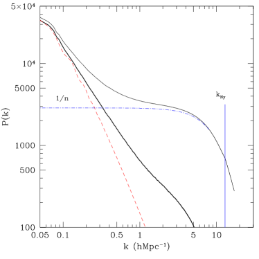
To estimate power spectra, we use a large density mesh of cells and then we apply the standard FFT method. The Cloud-In-Cell density assignment scheme is used to calculate the density fields from the coordinates of haloes in the simulations. However, before the power spectra can be reliably used two corrections should be applied: a correction due to the density assignment (Jing, 2005) and the usual shot-noise correction. If the number density of objects is and the Nyquist wave-number is , then the corrected power spectrum is given by
| (10) |
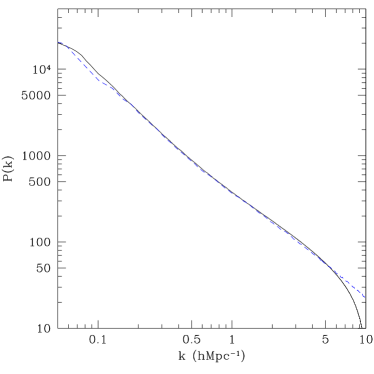
where is the length of the computational box and . This approximation is known to work well for (Jing, 2005; Cui et al., 2008). However, to remain on safe grounds we decided to limit our analysis to . The left panel of Fig. 11 illustrates the procedure of shot-noise and density corrections using a halo sample with km s-1 extracted from the MultiDark simulation at .
In the right panel of Fig. 11 we compare results of the MultiDark and Bolshoi simulations. Just as one may expect, there are some deviations at long waves due to the cosmic variance: the Bolshoi box of is too small to accurately probe these waves. There are also deviations at short waves that correspond to that are mainly due to the difference in density assignment between both simulations. For the Bolshoi simulation, the adopted mesh sets a minimum physical scale four times higher in frequency in comparison to MultiDark. However, for wave-numbers in the range the agreement between the simulations is remarkably good. This agreement is especially important for short waves, where both resolution and shot-noise could have corrupted the results. However, since this has not happened, it indicates that our power spectrum estimates for MultiDark can be trusted up to, at least, .
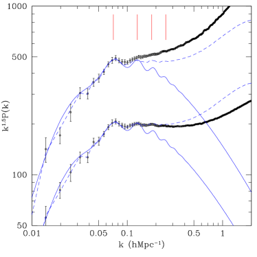
Fig. 12 shows power spectra of haloes with circular velocity cuts (top curves) and (bottom curves). To highlight BAO features, we actually plot the power spectra of the halo distribution multiplied by . As a result, the first five peaks in the spectra are clearly seen in the plot. However, they are somewhat smeared out by the non-linear evolution. As expected, the smearing increases for larger wave-numbers where the non-linearity is more important.
6.2.2 Abundance-matched halo bias
In what follows, we define the bias factor by
| (11) |
where is the linear power spectrum of the dark matter and is the power spectrum of haloes and subhaloes with circular velocities larger than . In order to distinguish the latter from the oftenly used non-linear dark matter power spectrum or from the power spectrum of distinct haloes only, we use subscript HAM to indicate that the results correspond to our HAM technique. By definition, the scale-dependent bias factor of Eq. (11) encodes the information of the non-linear power spectrum of the “galaxy” sample.
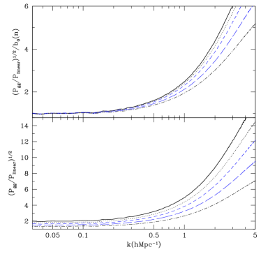
We start our analysis with the long-wave normalization of the bias parameter for different peak velocity cuts and, thus, for different number densities of our “galaxies”. The bottom panel in Fig. 13 shows for different velocities; at all wave-numbers it increases with increasing . The top panel shows that when normalized to the long-wave value, , the bias factor is nearly the same. However, there is some residual dependence on , i.e., the deviations of the bias from one velocity cut to another can be as large as 15% and this should be taken into account if an accurate fit is needed. An approximation for the real-space long-wave bias factor as a function of the average number density of dark matter haloes, , is presented below:
| (12) |
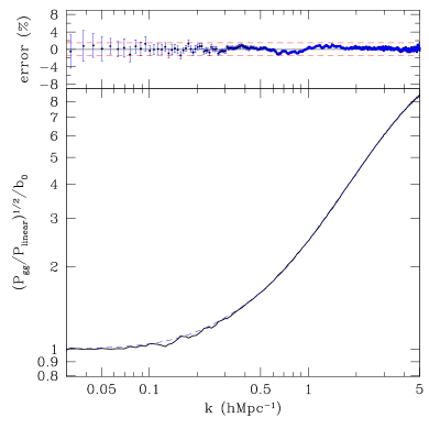
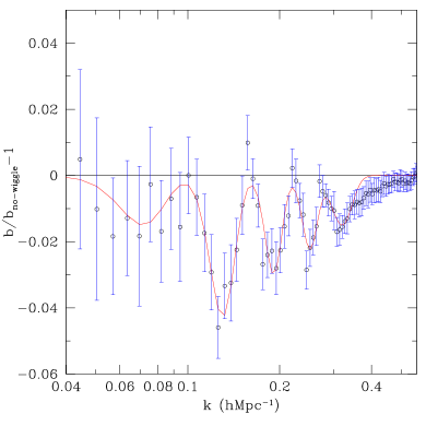
where is in units of . We now focus our analysis on the bias factor of haloes with , whose abundance is close that of BOSS-CMASS galaxies at . The top panel of Fig. 14 shows the bias factor of these haloes normalized to the value found at long waves, i.e. . Overall the bias factor is nearly flat at long waves and monotonically increases to short waves. The following approximation for the smooth (i.e., “de-wiggled”) component of gives percent-level accuracy (see dashed line in the top panel (bottom plot) of Fig. 14):
| (13) |
where the wave-number is in units of and the subscript ‘dw’ stands for ‘de-wiggled’. However, this approximation misses an important effect of non-linearities: the damping of the BAO signal in Fourier-space. The coupling between different Fourier modes washes out the acoustic oscillations, erasing the higher harmonic peaks (Meiksin et al., 1999; Eisenstein et al., 2007b; Angulo et al., 2005, 2008; Sánchez et al., 2008; Montesano et al., 2010). In recent years, there has been substantial progress in the theoretical understanding of non-linear distortions in the BAO signal, which can now be accurately modelled (see e.g., Crocce & Scoccimarro, 2006, 2008; Matsubara, 2008b, a; Taruya et al., 2009), and even partially corrected for (Eisenstein et al., 2007a; Seo et al., 2010). As the bias factor in Eq. (11) is defined with respect to the extrapolated linear theory power spectrum, this damping leads to small wiggles in the bias at the 2–4% level detected at high significance for (see bottom panel of Fig. 14). Therefore, in order to improve the fitting of the bias we also included the five main BAO peaks on top of the smooth component as follows:
| (14) |
Here each BAO peak is approximated as a small suppression of the bias factor given by the last term of the equation, is the wave-number of the peak and – and – are free parameters. The typical errors given by this approximation are smaller than 2% (see the top panel (top plot) of Fig. 14). The values of the parameters used in the equation can be seen in Table 1.
| BAO peak | |||
|---|---|---|---|
| 1 | 0.071 | 0.015 | 0.017 |
| 2 | 0.130 | 0.043 | 0.017 |
| 3 | 0.191 | 0.030 | 0.017 |
| 4 | 0.251 | 0.022 | 0.020 |
| 5 | 0.310 | 0.015 | 0.035 |
7 Conclusions
We presented an analysis of the clustering of galaxies in the DR9 sample of BOSS data for a wide range of scales ranging from to . We separately studied the clustering in the northern and southern hemispheres, as well as for the combined sky sample. We measured the two-dimensional, projected and redshift-space correlation functions and compare the results with those obtained from a large cosmological simulation with on a side at a redshift of . We also provide tables of the measured correlations together with estimates of the correlation matrices of the observed correlations (see Appendix B). The cosmological parameters adopted in the simulation are consistent with the latest WMAP7 results and several other probes. To bridge the gap between galaxies and dark matter haloes we use an HAM technique applied to the BOSS-CMASS sample. Our simulation, also known as MultiDark, is able to resolve the relevant subhalo masses needed to analyse the resulting satellite distribution. It is worth noting that the subhalo population in the simulation is completely determined by the cosmological model adopted not relying on a pure fit to the empirical correlation functions.
Our main results can be summarized as follows:
-
•
There is a 10–20% asymmetry in the projected and redshift-space correlation functions between the north and south subsamples at scales, which is better seen in the case of the projected correlation function. However, for both subsamples, the mean values agree with each other within a level of uncertainty.
-
•
As compared with the first-semester of BOSS results presented by White et al. (2011), we find a small increase in power in the projected correlation function at scales smaller than due to the improved treatment of fibre collisions and new corrections for systematics. However, the correlation functions (projected and redshift-space) decline by 10–20% at – scales in comparison with our HAM model. This is most noticeable for the north subsample which has about four times larger statistics than its southern counterpart. The comparison with the south subsample yields more consistent results with MultiDark at all scales, both in the projected and redshift-space correlations.
-
•
Our -body results for the clustering of “galaxies” give a reasonable representation of the measured clustering in the CMASS sample given the simplicity of the HAM model used. The more consistent results between the north and south subsamples for the redshift-space correlation function show a remarkable agreement with theory on scales ranging from up to : the differences are of the order of . This result is more impressive when considering the fact that our simple HAM scheme does not include any free parameter. However, for our matching tends to overpredict the clustering amplitude given by observations. Additionally, at distances in the range – we find some deviations () when comparing the model to the combined galaxy sample. Statistically, this difference is important – e.g., it represents a deviation at . Future data and a more sophisticated theoretical modelling may help to clarify the situation.
-
•
The distribution of (sub)haloes as a function of halo mass, as measured from our abundance-matched halo catalogue, points towards a galaxy population inhabiting haloes of mass M☉, with about of them being satellites orbiting centrals with M☉. We also derived values for the HOD parameters of the sample using our simulation, i.e. and .
-
•
The scale-dependent real-space galaxy bias of BOSS-CMASS galaxies is likely to be at scales Mpc (see Eq. (9)) as inferred both from the HAM and BOSS-CMASS observed correlations (see Fig. 10). Furthermore, using our simulation, we also computed a large-scale bias (defined as the ratio between the abundance-matched galaxy catalogue and the extrapolated linear matter power spectra; see Eq. (11)) and found that it depends on the “galaxy” number density as for the cosmological model adopted in our simulation. Specifically, for a (sub)halo number density of , we get .
-
•
The large-scale galaxy bias, defined using Eq. (11), has –4% dips at the positions of BAO peaks in the spectrum of fluctuations that are due to shifts caused by non-linear effects. In this case, we also provide a formula of the bias as a function of number density for the cosmology adopted here that can also be used to recover the non-linear “galaxy” power spectrum in terms of the extrapolated linear density field of matter.
Acknowledgments
We thank the anonymous referee for several comments that helped to improve this work.
Funding for SDSS-III has been provided by the Alfred P. Sloan Foundation, the Participating Institutions, the National Science Foundation, and the U.S. Department of Energy. SDSS-III is managed by the Astrophysical Research Consortium for the Participating Institutions of the SDSS-III Collaboration including the University of Arizona, the Brazilian Participation Group, Brookhaven National Laboratory, University of Cambridge, University of Florida, the French Participation Group, the German Participation Group, the Instituto de Astrofisica de Canarias, the Michigan State/Notre Dame/JINA Participation Group, Johns Hopkins University, Lawrence Berkeley National Laboratory, Max Planck Institute for Astrophysics, New Mexico State University, New York University, Ohio State University, Pennsylvania State University, University of Portsmouth, Princeton University, the Spanish Participation Group, University of Tokyo, University of Utah, Vanderbilt University, University of Virginia, University of Washington, and Yale University.
The MultiDark Database used in this paper and the web application providing online access to it were constructed as part of the activities of the German Astrophysical Virtual Observatory as a result of the collaboration between the Leibniz-Institute for Astrophysics Potsdam (AIP) and the Spanish MultiDark Consolider Project CSD2009-00064. The Bolshoi and MultiDark simulations were run on the NASA’s Pleiades supercomputer at the NASA Ames Research Center.
S.E.N. and F.P. acknowledges support from the Spanish MICINN’s Consolider grant MultiDark CSD2009-00064. S.E.N. also acknowledges support by the Deutsche Forschungsgemeinschaft under the grant MU1020 16-1. F.P. also thanks the support of the MICINN Spanish grant AYA2010-21231-C02-01 and the Campus of International Excellence UAMCSIC. A.K. acknowledges support from the NSF under a grant to NMSU.
References
- Abazajian et al. (2005) Abazajian, K., et al. 2005, ApJ, 625, 613
- Ahn et al. (2012) Ahn, C. P., et al. 2012, ApJS, 203, 21
- Anderson et al. (2012) Anderson, L., et al. 2012, MNRAS, 427, 3435
- Angulo et al. (2005) Angulo, R., Baugh, C. M., Frenk, C. S., Bower, R. G., Jenkins, A., & Morris, S. L. 2005, MNRAS, 362, L25
- Angulo et al. (2008) Angulo, R. E., Baugh, C. M., Frenk, C. S., & Lacey, C. G. 2008, MNRAS, 383, 755
- Behroozi et al. (2010) Behroozi, P. S., Conroy, C., & Wechsler, R. H. 2010, ApJ, 717, 379
- Behroozi et al. (2013) Behroozi, P. S., Wechsler, R. H., Wu, H.-Y., Busha, M. T., Klypin, A. A., & Primack, J. R. 2013, ApJ, 763, 18
- Berlind & Weinberg (2002) Berlind, A. A., & Weinberg, D. H. 2002, ApJ, 575, 587
- Blake et al. (2008) Blake, C., Collister, A., & Lahav, O. 2008, MNRAS, 385, 1257
- Blanton et al. (2003) Blanton, M. R., Lin, H., Lupton, R. H., Maley, F. M., Young, N., Zehavi, I., & Loveday, J. 2003, AJ, 125, 2276
- Bolton et al. (2012) Bolton, A. S., et al. 2012, AJ, 144, 144
- Brown et al. (2008) Brown, M. J. I., et al. 2008, ApJ, 682, 937
- Colless et al. (2001) Colless, M., et al. 2001, MNRAS, 328, 1039
- Conroy et al. (2006) Conroy, C., Wechsler, R. H., & Kravtsov, A. V. 2006, ApJ, 647, 201
- Crocce & Scoccimarro (2006) Crocce, M., & Scoccimarro, R. 2006, PRD, 73, 063519
- Crocce & Scoccimarro (2008) —. 2008, PRD, 77, 023533
- Cui et al. (2008) Cui, W., Liu, L., Yang, X., Wang, Y., Feng, L., & Springel, V. 2008, ApJ, 687, 738
- Davis & Peebles (1983) Davis, M., & Peebles, P. J. E. 1983, ApJ, 267, 465
- Dawson et al. (2013) Dawson, K. S., et al. 2013, AJ, 145, 10
- Eisenstein et al. (2007a) Eisenstein, D. J., Seo, H.-J., Sirko, E., & Spergel, D. N. 2007a, ApJ, 664, 675
- Eisenstein et al. (2007b) Eisenstein, D. J., Seo, H.-J., & White, M. 2007b, ApJ, 664, 660
- Eisenstein et al. (2011) Eisenstein, D. J., et al. 2011, AJ, 142, 72
- Fukugita et al. (1996) Fukugita, M., Ichikawa, T., Gunn, J. E., Doi, M., Shimasaku, K., & Schneider, D. P. 1996, AJ, 111, 1748
- Gottlöber & Klypin (2008) Gottlöber, S., & Klypin, A. 2008, ArXiv e-prints
- Gunn et al. (1998) Gunn, J. E., et al. 1998, AJ, 116, 3040
- Gunn et al. (2006) —. 2006, AJ, 131, 2332
- Guo et al. (2012) Guo, H., Zehavi, I., & Zheng, Z. 2012, ApJ, 756, 127
- Guo et al. (2010) Guo, Q., White, S., Li, C., & Boylan-Kolchin, M. 2010, MNRAS, 404, 1111
- Hamilton (1993) Hamilton, A. J. S. 1993, ApJ, 417, 19
- Hamilton & Tegmark (2004) Hamilton, A. J. S., & Tegmark, M. 2004, MNRAS, 349, 115
- Ho et al. (2012) Ho, S., et al. 2012, ApJ, 761, 14
- Jarosik et al. (2011) Jarosik, N., et al. 2011, ApJS, 192, 14
- Jing (2005) Jing, Y. P. 2005, ApJ, 620, 559
- Kaiser (1987) Kaiser, N. 1987, MNRAS, 227, 1
- Kim et al. (2008) Kim, J., Park, C., & Choi, Y.-Y. 2008, ApJ, 683, 123
- Klypin & Holtzman (1997) Klypin, A., & Holtzman, J. 1997, ArXiv Astrophysics e-prints
- Klypin et al. (2002) Klypin, A., Zhao, H., & Somerville, R. S. 2002, ApJ, 573, 597
- Klypin et al. (2011) Klypin, A. A., Trujillo-Gomez, S., & Primack, J. 2011, ApJ, 740, 102
- Knebe et al. (2011) Knebe, A., et al. 2011, MNRAS, 415, 2293
- Kravtsov et al. (2004) Kravtsov, A. V., Berlind, A. A., Wechsler, R. H., Klypin, A. A., Gottlöber, S., Allgood, B., & Primack, J. R. 2004, ApJ, 609, 35
- Kravtsov et al. (1997) Kravtsov, A. V., Klypin, A. A., & Khokhlov, A. M. 1997, ApJS, 111, 73
- Kulkarni et al. (2007) Kulkarni, G. V., Nichol, R. C., Sheth, R. K., Seo, H.-J., Eisenstein, D. J., & Gray, A. 2007, MNRAS, 378, 1196
- Landy & Szalay (1993) Landy, S. D., & Szalay, A. S. 1993, ApJ, 412, 64
- Leauthaud et al. (2011) Leauthaud, A., Tinker, J., Behroozi, P. S., Busha, M. T., & Wechsler, R. H. 2011, ApJ, 738, 45
- Li & White (2009) Li, C., & White, S. D. M. 2009, MNRAS, 398, 2177
- Mandelbaum et al. (2006) Mandelbaum, R., Seljak, U., Kauffmann, G., Hirata, C. M., & Brinkmann, J. 2006, MNRAS, 368, 715
- Manera et al. (2013) Manera, M., et al. 2013, MNRAS, 428, 1036
- Masjedi et al. (2006) Masjedi, M., et al. 2006, ApJ, 644, 54
- Masters et al. (2011) Masters, K. L., et al. 2011, MNRAS, 418, 1055
- Matsubara (2008a) Matsubara, T. 2008a, PRD, 78, 083519
- Matsubara (2008b) —. 2008b, PRD, 77, 063530
- Meiksin et al. (1999) Meiksin, A., White, M., & Peacock, J. A. 1999, MNRAS, 304, 851
- Montesano et al. (2010) Montesano, F., Sánchez, A. G., & Phleps, S. 2010, MNRAS, 408, 2397
- Padmanabhan et al. (2009) Padmanabhan, N., White, M., Norberg, P., & Porciani, C. 2009, MNRAS, 397, 1862
- Phleps et al. (2006) Phleps, S., Peacock, J. A., Meisenheimer, K., & Wolf, C. 2006, A&A, 457, 145
- Prada et al. (2012) Prada, F., Klypin, A. A., Cuesta, A. J., Betancort-Rijo, J. E., & Primack, J. 2012, MNRAS, 423, 3018
- Reddick et al. (2012) Reddick, R. M., Wechsler, R. H., Tinker, J. L., & Behroozi, P. S. 2012, ArXiv e-prints
- Reid et al. (2012) Reid, B. A., et al. 2012, MNRAS, 426, 2719
- Riebe et al. (2011) Riebe, K., et al. 2011, ArXiv e-prints
- Ross & Brunner (2009) Ross, A. J., & Brunner, R. J. 2009, MNRAS, 399, 878
- Ross et al. (2010) Ross, A. J., Percival, W. J., & Brunner, R. J. 2010, MNRAS, 407, 420
- Ross et al. (2011) Ross, A. J., et al. 2011, MNRAS, 417, 1350
- Ross et al. (2012) —. 2012, MNRAS, 424, 564
- Ross et al. (2007) Ross, N. P., et al. 2007, MNRAS, 381, 573
- Sánchez et al. (2008) Sánchez, A. G., Baugh, C. M., & Angulo, R. 2008, MNRAS, 390, 1470
- Sánchez et al. (2012) Sánchez, A. G., et al. 2012, MNRAS, 425, 415
- Schlafly & Finkbeiner (2011) Schlafly, E. F., & Finkbeiner, D. P. 2011, ApJ, 737, 103
- Schlafly et al. (2010) Schlafly, E. F., Finkbeiner, D. P., Schlegel, D. J., Jurić, M., Ivezić, Ž., Gibson, R. R., Knapp, G. R., & Weaver, B. A. 2010, ApJ, 725, 1175
- Scoccimarro & Sheth (2002) Scoccimarro, R., & Sheth, R. K. 2002, MNRAS, 329, 629
- Seo et al. (2010) Seo, H.-J., Eckel, J., Eisenstein, D. J., Mehta, K., Metchnik, M., Padmanabhan, N., Pinto, P., Takahashi, R., et al. 2010, ApJ, 720, 1650
- Skibba & Sheth (2009) Skibba, R. A., & Sheth, R. K. 2009, MNRAS, 392, 1080
- Slosar et al. (2011) Slosar, A., et al. 2011, JCAP, 9, 1
- Smee et al. (2012) Smee, S., et al. 2012, ArXiv e-prints
- Swanson et al. (2008) Swanson, M. E. C., Tegmark, M., Hamilton, A. J. S., & Hill, J. C. 2008, MNRAS, 387, 1391
- Taruya et al. (2009) Taruya, A., Nishimichi, T., Saito, S., & Hiramatsu, T. 2009, PRD, 80, 123503
- Tasitsiomi et al. (2004) Tasitsiomi, A., Kravtsov, A. V., Gottlöber, S., & Klypin, A. A. 2004, ApJ, 607, 125
- Tegmark et al. (2004) Tegmark et al., M. 2004, ApJ, 606, 702
- Trujillo-Gomez et al. (2011) Trujillo-Gomez, S., Klypin, A., Primack, J., & Romanowsky, A. J. 2011, ApJ, 742, 16
- Vale & Ostriker (2004) Vale, A., & Ostriker, J. P. 2004, MNRAS, 353, 189
- Wake et al. (2008) Wake, D. A., Croom, S. M., Sadler, E. M., & Johnston, H. M. 2008, MNRAS, 391, 1674
- Watson et al. (2012) Watson, D. F., Berlind, A. A., & Zentner, A. R. 2012, ApJ, 754, 90
- Wetzel & White (2010) Wetzel, A. R., & White, M. 2010, MNRAS, 403, 1072
- White et al. (2011) White, M., et al. 2011, ApJ, 728, 126
- York et al. (2000) York, D. G., et al. 2000, AJ, 120, 1579
- Zehavi et al. (2002) Zehavi, I., et al. 2002, ApJ, 571, 172
- Zehavi et al. (2005) —. 2005, ApJ, 630, 1
- Zehavi et al. (2011) —. 2011, ApJ, 736, 59
- Zentner et al. (2005) Zentner, A. R., Berlind, A. A., Bullock, J. S., Kravtsov, A. V., & Wechsler, R. H. 2005, ApJ, 624, 505
- Zheng et al. (2009) Zheng, Z., Zehavi, I., Eisenstein, D. J., Weinberg, D. H., & Jing, Y. P. 2009, ApJ, 707, 554
- Zheng et al. (2005) Zheng, Z., et al. 2005, ApJ, 633, 791
Appendix A Dependence of clustering on different effects
A.1 Halo finding
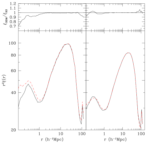
The dependence of clustering with the halo finder used to identify virialized systems in the simulation is shown in Fig. 15 for the BDM (Klypin & Holtzman, 1997; Riebe et al., 2011) and RockStar (Behroozi et al., 2013) codes. As an example we select all (sub)haloes present in the Multidark simulation at with V km s-1 and V km s-1 in order to compute the real-space correlation function of the resulting halo catalogues. As can be seen in the figure the convergence between both halo finders is remarkable; for small (i.e., –) and large (i.e., ) scales the differences in power are typically of the order of .
A.2 Redshift evolution of BOSS-CMASS galaxies
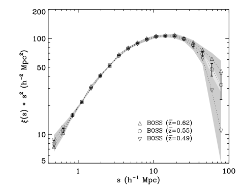
To assess the evolution of clustering with redshift within the BOSS-CMASS sample we splitted the combined (north+south) sample into three different subsamples with mean redshifts of chosen to be around our fiducial value of . Fig. 16 shows that the clustering power is essentially independent of the corresponding mean redshift of the BOSS-CMASS sample for a large range of scales: the differences are negligible within the range – but tend to increase for smaller and larger scales. At the largest scales the measurements of the subsample at show the largest deviations in amplitude, as well as in the errors due to the smaller volume probed. However, the different correlation functions are still compatible with each other since deviations are within the level given by cosmic variance, as indicated by the error bars and shaded areas (see Section 3.3).
A.3 Halo number density
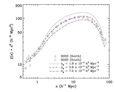
To assess the clustering dependence with number density we evaluate different redshift-space correlations and compare with observations (see Fig. 17). We compute three different correlation functions using the MultiDark halo catalogues at assuming the stochasticity model presented in Section 3.2. We use the following number densities: . The dashed line corresponds to our effective number density, i.e. . As expected, doubling and dividing results in a weaker and stronger clustering signal respectively. In these extreme cases, the departure from observed BOSS-CMASS number densities at the peak of the redshift distribution is typically above observational uncertainties. However, at , typical departures from the effective number density adopted in this work (e.g., between north and south subsamples) are smaller than 5% and do not appreciably change our final result.
Appendix B Tables of correlation functions and covariances
| 0.553 | 306.519 | 258.526 | 296.364 | 270.370 | 10.593 | 21.021 | 9.409 | 6.636 |
|---|---|---|---|---|---|---|---|---|
| 0.704 | 233.934 | 205.410 | 227.127 | 199.688 | 7.999 | 14.564 | 6.947 | 4.072 |
| 0.896 | 174.314 | 189.613 | 177.940 | 154.041 | 6.279 | 12.604 | 5.552 | 3.314 |
| 1.142 | 136.240 | 128.103 | 134.317 | 129.333 | 4.887 | 9.055 | 4.262 | 2.935 |
| 1.454 | 110.571 | 122.007 | 113.243 | 105.771 | 3.933 | 7.166 | 3.422 | 1.790 |
| 1.851 | 93.106 | 91.557 | 92.791 | 88.003 | 3.203 | 5.809 | 2.780 | 1.797 |
| 2.358 | 77.150 | 79.987 | 77.836 | 76.210 | 2.846 | 4.852 | 2.403 | 1.364 |
| 3.003 | 67.574 | 68.062 | 67.713 | 65.581 | 2.174 | 3.944 | 1.884 | 1.534 |
| 3.824 | 55.136 | 55.377 | 55.221 | 55.377 | 1.857 | 3.498 | 1.604 | 1.325 |
| 4.870 | 43.813 | 45.420 | 44.212 | 46.636 | 1.567 | 2.951 | 1.356 | 1.168 |
| 6.202 | 37.769 | 40.875 | 38.522 | 39.079 | 1.410 | 2.567 | 1.208 | 1.036 |
| 7.898 | 29.486 | 30.329 | 29.667 | 31.701 | 1.184 | 2.273 | 1.022 | 0.996 |
| 10.058 | 24.699 | 25.506 | 24.906 | 25.899 | 1.092 | 1.998 | 0.931 | 0.962 |
| 12.809 | 18.341 | 19.348 | 18.572 | 19.582 | 1.043 | 1.807 | 0.873 | 0.938 |
| 16.312 | 13.561 | 14.853 | 13.842 | 15.044 | 0.913 | 1.634 | 0.771 | 0.884 |
| 20.773 | 9.455 | 10.960 | 9.779 | 10.777 | 0.809 | 1.437 | 0.677 | 0.831 |
| 26.455 | 6.833 | 7.845 | 7.051 | 7.253 | 0.741 | 1.358 | 0.625 | 0.714 |
| 33.690 | 4.465 | 5.390 | 4.656 | 4.654 | 0.663 | 1.182 | 0.553 | 0.625 |
| 42.904 | 2.789 | 3.289 | 2.888 | 2.925 | 0.599 | 1.058 | 0.491 | 0.502 |
| 54.639 | 1.827 | 2.399 | 1.941 | 1.393 | 0.520 | 0.957 | 0.420 | 0.406 |
| 69.582 | 1.496 | 1.468 | 1.480 | 0.863 | 0.463 | 0.821 | 0.361 | 0.387 |
| 88.614 | 1.087 | 0.975 | 1.059 | 0.835 | 0.429 | 0.745 | 0.324 | 0.317 |
| 0.476 | 37.266 | 35.725 | 37.880 | 55.002 | 5.733 | 10.891 | 5.260 | 1.071 |
|---|---|---|---|---|---|---|---|---|
| 0.632 | 29.886 | 23.598 | 28.942 | 37.425 | 2.809 | 5.442 | 2.477 | 0.623 |
| 0.839 | 22.851 | 23.385 | 23.270 | 24.742 | 1.399 | 2.595 | 1.243 | 0.510 |
| 1.114 | 17.698 | 18.450 | 18.003 | 17.917 | 0.683 | 1.182 | 0.604 | 0.223 |
| 1.479 | 14.595 | 12.877 | 14.314 | 13.837 | 0.348 | 0.644 | 0.307 | 0.153 |
| 1.965 | 10.598 | 10.881 | 10.725 | 10.508 | 0.196 | 0.374 | 0.174 | 0.088 |
| 2.609 | 7.843 | 7.095 | 7.705 | 7.910 | 0.118 | 0.207 | 0.107 | 0.059 |
| 3.464 | 5.590 | 5.464 | 5.585 | 5.627 | 0.067 | 0.134 | 0.066 | 0.039 |
| 4.600 | 3.736 | 3.733 | 3.744 | 3.789 | 0.039 | 0.075 | 0.038 | 0.029 |
| 6.108 | 2.375 | 2.416 | 2.392 | 2.438 | 0.026 | 0.046 | 0.024 | 0.016 |
| 8.111 | 1.494 | 1.469 | 1.493 | 1.532 | 0.016 | 0.031 | 0.015 | 0.012 |
| 10.771 | 0.906 | 0.896 | 0.906 | 0.936 | 0.011 | 0.021 | 0.010 | 0.009 |
| 14.303 | 0.521 | 0.516 | 0.521 | 0.559 | 0.008 | 0.015 | 0.007 | 0.007 |
| 18.993 | 0.294 | 0.299 | 0.296 | 0.323 | 0.006 | 0.012 | 0.005 | 0.005 |
| 25.221 | 0.152 | 0.168 | 0.156 | 0.179 | 0.005 | 0.009 | 0.004 | 0.004 |
| 33.491 | 0.075 | 0.083 | 0.077 | 0.093 | 0.004 | 0.007 | 0.003 | 0.003 |
| 44.473 | 0.035 | 0.037 | 0.035 | 0.041 | 0.003 | 0.006 | 0.003 | 0.002 |
| 59.056 | 0.014 | 0.015 | 0.014 | 0.014 | 0.002 | 0.004 | 0.002 | 0.002 |
| 78.421 | 0.006 | 0.005 | 0.006 | 0.005 | 0.002 | 0.003 | 0.002 | 0.002 |
| 0.553 | 0.704 | 0.896 | 1.142 | 1.454 | 1.851 | 2.358 | 3.003 | 3.824 | 4.870 | 6.202 | 7.898 | 10.058 | 12.809 | 16.312 | 20.773 | 26.455 | 33.690 | 42.904 | 54.639 | 69.582 | 88.614 | |
|---|---|---|---|---|---|---|---|---|---|---|---|---|---|---|---|---|---|---|---|---|---|---|
| 0.553 | 1.000 | – | – | – | – | – | – | – | – | – | – | – | – | – | – | – | – | – | – | – | – | – |
| 0.704 | 0.112 | 1.000 | – | – | – | – | – | – | – | – | – | – | – | – | – | – | – | – | – | – | – | – |
| 0.896 | 0.072 | 0.105 | 1.000 | – | – | – | – | – | – | – | – | – | – | – | – | – | – | – | – | – | – | – |
| 1.142 | 0.129 | 0.070 | 0.151 | 1.000 | – | – | – | – | – | – | – | – | – | – | – | – | – | – | – | – | – | – |
| 1.454 | 0.030 | 0.135 | 0.096 | 0.174 | 1.000 | – | – | – | – | – | – | – | – | – | – | – | – | – | – | – | – | – |
| 1.851 | 0.034 | 0.149 | 0.147 | 0.127 | 0.152 | 1.000 | – | – | – | – | – | – | – | – | – | – | – | – | – | – | – | – |
| 2.358 | 0.111 | 0.211 | 0.134 | 0.167 | 0.215 | 0.255 | 1.000 | – | – | – | – | – | – | – | – | – | – | – | – | – | – | – |
| 3.003 | 0.142 | 0.146 | 0.146 | 0.142 | 0.218 | 0.204 | 0.352 | 1.000 | – | – | – | – | – | – | – | – | – | – | – | – | – | – |
| 3.824 | 0.069 | 0.117 | 0.112 | 0.185 | 0.162 | 0.311 | 0.370 | 0.408 | 1.000 | – | – | – | – | – | – | – | – | – | – | – | – | – |
| 4.870 | 0.102 | 0.086 | 0.153 | 0.170 | 0.216 | 0.208 | 0.374 | 0.332 | 0.402 | 1.000 | – | – | – | – | – | – | – | – | – | – | – | – |
| 6.202 | 0.118 | 0.101 | 0.179 | 0.184 | 0.208 | 0.264 | 0.379 | 0.411 | 0.467 | 0.504 | 1.000 | – | – | – | – | – | – | – | – | – | – | – |
| 7.898 | 0.131 | 0.113 | 0.156 | 0.197 | 0.241 | 0.291 | 0.453 | 0.407 | 0.461 | 0.522 | 0.648 | 1.000 | – | – | – | – | – | – | – | – | – | – |
| 10.058 | 0.114 | 0.104 | 0.155 | 0.229 | 0.277 | 0.290 | 0.442 | 0.401 | 0.488 | 0.518 | 0.656 | 0.710 | 1.000 | – | – | – | – | – | – | – | – | – |
| 12.809 | 0.104 | 0.149 | 0.190 | 0.221 | 0.254 | 0.288 | 0.436 | 0.388 | 0.456 | 0.499 | 0.627 | 0.685 | 0.788 | 1.000 | – | – | – | – | – | – | – | – |
| 16.312 | 0.119 | 0.163 | 0.179 | 0.242 | 0.228 | 0.288 | 0.400 | 0.367 | 0.456 | 0.481 | 0.583 | 0.633 | 0.771 | 0.812 | 1.000 | – | – | – | – | – | – | – |
| 20.773 | 0.115 | 0.152 | 0.157 | 0.192 | 0.192 | 0.248 | 0.364 | 0.363 | 0.419 | 0.427 | 0.553 | 0.602 | 0.720 | 0.761 | 0.837 | 1.000 | – | – | – | – | – | – |
| 26.455 | 0.095 | 0.152 | 0.141 | 0.182 | 0.191 | 0.204 | 0.336 | 0.337 | 0.370 | 0.410 | 0.526 | 0.579 | 0.664 | 0.698 | 0.768 | 0.856 | 1.000 | – | – | – | – | – |
| 33.690 | 0.086 | 0.093 | 0.101 | 0.178 | 0.165 | 0.179 | 0.281 | 0.292 | 0.325 | 0.364 | 0.472 | 0.495 | 0.592 | 0.597 | 0.677 | 0.737 | 0.838 | 1.000 | – | – | – | – |
| 42.904 | 0.084 | 0.077 | 0.086 | 0.208 | 0.142 | 0.147 | 0.260 | 0.254 | 0.282 | 0.326 | 0.408 | 0.438 | 0.513 | 0.509 | 0.592 | 0.646 | 0.735 | 0.857 | 1.000 | – | – | – |
| 54.639 | 0.074 | 0.035 | 0.071 | 0.198 | 0.121 | 0.106 | 0.247 | 0.229 | 0.220 | 0.258 | 0.338 | 0.357 | 0.414 | 0.411 | 0.489 | 0.525 | 0.617 | 0.711 | 0.843 | 1.000 | – | – |
| 69.582 | 0.013 | 0.002 | 0.078 | 0.144 | 0.111 | 0.030 | 0.170 | 0.178 | 0.175 | 0.196 | 0.261 | 0.320 | 0.323 | 0.318 | 0.376 | 0.397 | 0.491 | 0.567 | 0.671 | 0.820 | 1.000 | – |
| 88.614 | 0.028 | -0.016 | 0.026 | 0.082 | 0.064 | 0.001 | 0.138 | 0.136 | 0.135 | 0.131 | 0.162 | 0.248 | 0.236 | 0.255 | 0.292 | 0.311 | 0.372 | 0.423 | 0.519 | 0.608 | 0.787 | 1.000 |
| 0.553 | 0.704 | 0.896 | 1.142 | 1.454 | 1.851 | 2.358 | 3.003 | 3.824 | 4.870 | 6.202 | 7.898 | 10.058 | 12.809 | 16.312 | 20.773 | 26.455 | 33.690 | 42.904 | 54.639 | 69.582 | 88.614 | |
|---|---|---|---|---|---|---|---|---|---|---|---|---|---|---|---|---|---|---|---|---|---|---|
| 0.553 | 1.000 | – | – | – | – | – | – | – | – | – | – | – | – | – | – | – | – | – | – | – | – | – |
| 0.704 | 0.127 | 1.000 | – | – | – | – | – | – | – | – | – | – | – | – | – | – | – | – | – | – | – | – |
| 0.896 | 0.118 | 0.146 | 1.000 | – | – | – | – | – | – | – | – | – | – | – | – | – | – | – | – | – | – | – |
| 1.142 | 0.062 | 0.121 | 0.148 | 1.000 | – | – | – | – | – | – | – | – | – | – | – | – | – | – | – | – | – | – |
| 1.454 | 0.032 | 0.140 | 0.124 | 0.147 | 1.000 | – | – | – | – | – | – | – | – | – | – | – | – | – | – | – | – | – |
| 1.851 | 0.089 | 0.134 | 0.141 | 0.083 | 0.095 | 1.000 | – | – | – | – | – | – | – | – | – | – | – | – | – | – | – | – |
| 2.358 | 0.069 | 0.093 | 0.142 | 0.108 | 0.192 | 0.231 | 1.000 | – | – | – | – | – | – | – | – | – | – | – | – | – | – | – |
| 3.003 | 0.096 | 0.184 | 0.154 | 0.090 | 0.192 | 0.296 | 0.317 | 1.000 | – | – | – | – | – | – | – | – | – | – | – | – | – | – |
| 3.824 | 0.095 | 0.162 | 0.229 | 0.157 | 0.210 | 0.297 | 0.291 | 0.420 | 1.000 | – | – | – | – | – | – | – | – | – | – | – | – | – |
| 4.870 | 0.084 | 0.167 | 0.213 | 0.146 | 0.253 | 0.284 | 0.348 | 0.389 | 0.535 | 1.000 | – | – | – | – | – | – | – | – | – | – | – | – |
| 6.202 | 0.158 | 0.178 | 0.226 | 0.183 | 0.255 | 0.284 | 0.359 | 0.455 | 0.554 | 0.542 | 1.000 | – | – | – | – | – | – | – | – | – | – | – |
| 7.898 | 0.123 | 0.174 | 0.192 | 0.174 | 0.186 | 0.274 | 0.354 | 0.461 | 0.498 | 0.566 | 0.655 | 1.000 | – | – | – | – | – | – | – | – | – | – |
| 10.058 | 0.119 | 0.220 | 0.192 | 0.161 | 0.220 | 0.279 | 0.359 | 0.458 | 0.509 | 0.535 | 0.626 | 0.709 | 1.000 | – | – | – | – | – | – | – | – | – |
| 12.809 | 0.125 | 0.186 | 0.197 | 0.148 | 0.215 | 0.294 | 0.320 | 0.490 | 0.485 | 0.522 | 0.629 | 0.667 | 0.764 | 1.000 | – | – | – | – | – | – | – | – |
| 16.312 | 0.126 | 0.176 | 0.159 | 0.146 | 0.199 | 0.271 | 0.341 | 0.428 | 0.451 | 0.504 | 0.623 | 0.639 | 0.692 | 0.793 | 1.000 | – | – | – | – | – | – | – |
| 20.773 | 0.136 | 0.178 | 0.110 | 0.132 | 0.194 | 0.249 | 0.242 | 0.411 | 0.445 | 0.467 | 0.585 | 0.621 | 0.670 | 0.728 | 0.808 | 1.000 | – | – | – | – | – | – |
| 26.455 | 0.083 | 0.163 | 0.098 | 0.115 | 0.165 | 0.224 | 0.227 | 0.346 | 0.359 | 0.409 | 0.484 | 0.553 | 0.623 | 0.650 | 0.721 | 0.838 | 1.000 | – | – | – | – | – |
| 33.690 | 0.084 | 0.093 | 0.049 | 0.064 | 0.136 | 0.156 | 0.132 | 0.274 | 0.264 | 0.314 | 0.369 | 0.447 | 0.503 | 0.536 | 0.602 | 0.723 | 0.838 | 1.000 | – | – | – | – |
| 42.904 | 0.096 | 0.083 | -0.004 | 0.068 | 0.103 | 0.119 | 0.128 | 0.185 | 0.246 | 0.248 | 0.305 | 0.350 | 0.423 | 0.440 | 0.464 | 0.575 | 0.670 | 0.809 | 1.000 | – | – | – |
| 54.639 | 0.095 | 0.035 | -0.017 | 0.061 | 0.046 | 0.068 | 0.116 | 0.129 | 0.165 | 0.170 | 0.182 | 0.246 | 0.300 | 0.311 | 0.362 | 0.436 | 0.496 | 0.614 | 0.795 | 1.000 | – | – |
| 69.582 | 0.080 | 0.049 | 0.049 | 0.072 | 0.018 | 0.055 | 0.094 | 0.115 | 0.150 | 0.147 | 0.148 | 0.210 | 0.235 | 0.241 | 0.285 | 0.325 | 0.348 | 0.446 | 0.562 | 0.774 | 1.000 | – |
| 88.614 | 0.053 | 0.071 | 0.025 | 0.058 | 0.018 | 0.066 | 0.108 | 0.076 | 0.117 | 0.156 | 0.171 | 0.188 | 0.179 | 0.193 | 0.235 | 0.259 | 0.247 | 0.291 | 0.342 | 0.498 | 0.730 | 1.000 |
| 0.553 | 0.704 | 0.896 | 1.142 | 1.454 | 1.851 | 2.358 | 3.003 | 3.824 | 4.870 | 6.202 | 7.898 | 10.058 | 12.809 | 16.312 | 20.773 | 26.455 | 33.690 | 42.904 | 54.639 | 69.582 | 88.614 | |
|---|---|---|---|---|---|---|---|---|---|---|---|---|---|---|---|---|---|---|---|---|---|---|
| 0.553 | 1.000 | – | – | – | – | – | – | – | – | – | – | – | – | – | – | – | – | – | – | – | – | – |
| 0.704 | 0.114 | 1.000 | – | – | – | – | – | – | – | – | – | – | – | – | – | – | – | – | – | – | – | – |
| 0.896 | 0.079 | 0.105 | 1.000 | – | – | – | – | – | – | – | – | – | – | – | – | – | – | – | – | – | – | – |
| 1.142 | 0.109 | 0.079 | 0.144 | 1.000 | – | – | – | – | – | – | – | – | – | – | – | – | – | – | – | – | – | – |
| 1.454 | 0.030 | 0.135 | 0.098 | 0.163 | 1.000 | – | – | – | – | – | – | – | – | – | – | – | – | – | – | – | – | – |
| 1.851 | 0.042 | 0.139 | 0.141 | 0.112 | 0.141 | 1.000 | – | – | – | – | – | – | – | – | – | – | – | – | – | – | – | – |
| 2.358 | 0.092 | 0.178 | 0.124 | 0.139 | 0.204 | 0.242 | 1.000 | – | – | – | – | – | – | – | – | – | – | – | – | – | – | – |
| 3.003 | 0.127 | 0.152 | 0.139 | 0.119 | 0.209 | 0.226 | 0.339 | 1.000 | – | – | – | – | – | – | – | – | – | – | – | – | – | – |
| 3.824 | 0.064 | 0.114 | 0.127 | 0.168 | 0.168 | 0.300 | 0.337 | 0.407 | 1.000 | – | – | – | – | – | – | – | – | – | – | – | – | – |
| 4.870 | 0.088 | 0.098 | 0.150 | 0.151 | 0.221 | 0.221 | 0.356 | 0.337 | 0.421 | 1.000 | – | – | – | – | – | – | – | – | – | – | – | – |
| 6.202 | 0.120 | 0.114 | 0.176 | 0.172 | 0.212 | 0.266 | 0.360 | 0.418 | 0.476 | 0.495 | 1.000 | – | – | – | – | – | – | – | – | – | – | – |
| 7.898 | 0.123 | 0.119 | 0.149 | 0.176 | 0.220 | 0.286 | 0.414 | 0.410 | 0.455 | 0.518 | 0.639 | 1.000 | – | – | – | – | – | – | – | – | – | – |
| 10.058 | 0.107 | 0.123 | 0.146 | 0.196 | 0.260 | 0.285 | 0.409 | 0.406 | 0.480 | 0.506 | 0.641 | 0.698 | 1.000 | – | – | – | – | – | – | – | – | – |
| 12.809 | 0.098 | 0.152 | 0.177 | 0.191 | 0.239 | 0.288 | 0.387 | 0.404 | 0.449 | 0.488 | 0.617 | 0.666 | 0.774 | 1.000 | – | – | – | – | – | – | – | – |
| 16.312 | 0.111 | 0.165 | 0.158 | 0.203 | 0.215 | 0.281 | 0.363 | 0.370 | 0.440 | 0.471 | 0.580 | 0.617 | 0.745 | 0.799 | 1.000 | – | – | – | – | – | – | – |
| 20.773 | 0.109 | 0.156 | 0.132 | 0.159 | 0.182 | 0.250 | 0.312 | 0.363 | 0.410 | 0.419 | 0.550 | 0.585 | 0.697 | 0.740 | 0.822 | 1.000 | – | – | – | – | – | – |
| 26.455 | 0.084 | 0.155 | 0.116 | 0.148 | 0.177 | 0.209 | 0.286 | 0.325 | 0.351 | 0.392 | 0.504 | 0.550 | 0.639 | 0.670 | 0.746 | 0.842 | 1.000 | – | – | – | – | – |
| 33.690 | 0.075 | 0.094 | 0.074 | 0.131 | 0.148 | 0.175 | 0.219 | 0.271 | 0.292 | 0.333 | 0.433 | 0.455 | 0.551 | 0.559 | 0.642 | 0.715 | 0.826 | 1.000 | – | – | – | – |
| 42.904 | 0.071 | 0.081 | 0.049 | 0.157 | 0.121 | 0.144 | 0.197 | 0.220 | 0.253 | 0.288 | 0.369 | 0.386 | 0.465 | 0.461 | 0.539 | 0.603 | 0.700 | 0.835 | 1.000 | – | – | – |
| 54.639 | 0.059 | 0.033 | 0.029 | 0.147 | 0.089 | 0.098 | 0.176 | 0.185 | 0.178 | 0.205 | 0.275 | 0.286 | 0.348 | 0.339 | 0.421 | 0.460 | 0.556 | 0.662 | 0.812 | 1.000 | – | – |
| 69.582 | -0.001 | 0.007 | 0.045 | 0.100 | 0.071 | 0.030 | 0.098 | 0.133 | 0.131 | 0.140 | 0.192 | 0.239 | 0.248 | 0.231 | 0.297 | 0.313 | 0.405 | 0.492 | 0.600 | 0.775 | 1.000 | – |
| 88.614 | 0.004 | -0.007 | -0.016 | 0.033 | 0.025 | 0.004 | 0.063 | 0.079 | 0.081 | 0.076 | 0.103 | 0.161 | 0.149 | 0.154 | 0.198 | 0.209 | 0.263 | 0.319 | 0.402 | 0.501 | 0.718 | 1.000 |
| 0.476 | 0.632 | 0.839 | 1.114 | 1.479 | 1.965 | 2.609 | 3.464 | 4.600 | 6.108 | 8.111 | 10.771 | 14.303 | 18.993 | 25.221 | 33.491 | 44.473 | 59.056 | 78.421 | |
|---|---|---|---|---|---|---|---|---|---|---|---|---|---|---|---|---|---|---|---|
| 0.476 | 1.000 | – | – | – | – | – | – | – | – | – | – | – | – | – | – | – | – | – | – |
| 0.632 | 0.121 | 1.000 | – | – | – | – | – | – | – | – | – | – | – | – | – | – | – | – | – |
| 0.839 | 0.085 | 0.103 | 1.000 | – | – | – | – | – | – | – | – | – | – | – | – | – | – | – | – |
| 1.114 | 0.061 | 0.103 | 0.115 | 1.000 | – | – | – | – | – | – | – | – | – | – | – | – | – | – | – |
| 1.479 | 0.128 | 0.114 | 0.160 | 0.122 | 1.000 | – | – | – | – | – | – | – | – | – | – | – | – | – | – |
| 1.965 | 0.083 | 0.053 | 0.066 | 0.056 | 0.138 | 1.000 | – | – | – | – | – | – | – | – | – | – | – | – | – |
| 2.609 | 0.040 | -0.010 | 0.022 | 0.063 | 0.112 | 0.084 | 1.000 | – | – | – | – | – | – | – | – | – | – | – | – |
| 3.464 | 0.057 | 0.078 | 0.015 | 0.032 | 0.100 | 0.150 | 0.214 | 1.000 | – | – | – | – | – | – | – | – | – | – | – |
| 4.600 | 0.078 | 0.067 | 0.146 | 0.112 | 0.220 | 0.175 | 0.123 | 0.288 | 1.000 | – | – | – | – | – | – | – | – | – | – |
| 6.108 | 0.045 | 0.048 | 0.118 | 0.125 | 0.185 | 0.176 | 0.184 | 0.237 | 0.385 | 1.000 | – | – | – | – | – | – | – | – | – |
| 8.111 | 0.084 | 0.047 | 0.140 | 0.132 | 0.208 | 0.197 | 0.149 | 0.282 | 0.407 | 0.488 | 1.000 | – | – | – | – | – | – | – | – |
| 10.771 | 0.024 | 0.045 | 0.162 | 0.120 | 0.212 | 0.184 | 0.140 | 0.234 | 0.364 | 0.465 | 0.599 | 1.000 | – | – | – | – | – | – | – |
| 14.303 | 0.053 | 0.032 | 0.146 | 0.136 | 0.218 | 0.187 | 0.146 | 0.176 | 0.368 | 0.471 | 0.551 | 0.704 | 1.000 | – | – | – | – | – | – |
| 18.993 | 0.050 | 0.013 | 0.174 | 0.138 | 0.201 | 0.187 | 0.081 | 0.195 | 0.319 | 0.406 | 0.501 | 0.651 | 0.762 | 1.000 | – | – | – | – | – |
| 25.221 | 0.029 | -0.005 | 0.120 | 0.086 | 0.167 | 0.150 | 0.096 | 0.122 | 0.243 | 0.345 | 0.428 | 0.575 | 0.678 | 0.791 | 1.000 | – | – | – | – |
| 33.491 | -0.004 | -0.021 | 0.137 | 0.054 | 0.138 | 0.085 | 0.051 | 0.081 | 0.214 | 0.263 | 0.351 | 0.497 | 0.575 | 0.690 | 0.819 | 1.000 | – | – | – |
| 44.473 | 0.007 | -0.002 | 0.123 | 0.098 | 0.113 | 0.068 | 0.045 | 0.095 | 0.220 | 0.241 | 0.313 | 0.423 | 0.482 | 0.586 | 0.678 | 0.827 | 1.000 | – | – |
| 59.056 | -0.010 | 0.010 | 0.084 | 0.064 | 0.059 | 0.017 | 0.055 | 0.118 | 0.133 | 0.174 | 0.220 | 0.280 | 0.336 | 0.423 | 0.487 | 0.609 | 0.817 | 1.000 | – |
| 78.421 | -0.021 | 0.012 | 0.038 | 0.015 | 0.022 | 0.000 | 0.061 | 0.088 | 0.109 | 0.124 | 0.143 | 0.194 | 0.230 | 0.285 | 0.321 | 0.408 | 0.571 | 0.764 | 1.000 |
| 0.476 | 0.632 | 0.839 | 1.114 | 1.479 | 1.965 | 2.609 | 3.464 | 4.600 | 6.108 | 8.111 | 10.771 | 14.303 | 18.993 | 25.221 | 33.491 | 44.473 | 59.056 | 78.421 | |
|---|---|---|---|---|---|---|---|---|---|---|---|---|---|---|---|---|---|---|---|
| 0.476 | 1.000 | – | – | – | – | – | – | – | – | – | – | – | – | – | – | – | – | – | – |
| 0.632 | 0.053 | 1.000 | – | – | – | – | – | – | – | – | – | – | – | – | – | – | – | – | – |
| 0.839 | 0.080 | 0.102 | 1.000 | – | – | – | – | – | – | – | – | – | – | – | – | – | – | – | – |
| 1.114 | 0.123 | 0.081 | 0.143 | 1.000 | – | – | – | – | – | – | – | – | – | – | – | – | – | – | – |
| 1.479 | 0.039 | 0.034 | 0.040 | 0.014 | 1.000 | – | – | – | – | – | – | – | – | – | – | – | – | – | – |
| 1.965 | 0.006 | 0.031 | 0.081 | 0.129 | 0.072 | 1.000 | – | – | – | – | – | – | – | – | – | – | – | – | – |
| 2.609 | 0.019 | -0.041 | 0.097 | 0.016 | 0.126 | 0.107 | 1.000 | – | – | – | – | – | – | – | – | – | – | – | – |
| 3.464 | 0.006 | 0.100 | 0.144 | 0.137 | 0.054 | 0.141 | 0.216 | 1.000 | – | – | – | – | – | – | – | – | – | – | – |
| 4.600 | 0.031 | 0.126 | 0.123 | 0.114 | 0.079 | 0.125 | 0.126 | 0.276 | 1.000 | – | – | – | – | – | – | – | – | – | – |
| 6.108 | 0.080 | 0.095 | 0.186 | 0.123 | 0.120 | 0.153 | 0.198 | 0.284 | 0.344 | 1.000 | – | – | – | – | – | – | – | – | – |
| 8.111 | 0.108 | 0.098 | 0.098 | 0.155 | 0.130 | 0.119 | 0.179 | 0.295 | 0.321 | 0.487 | 1.000 | – | – | – | – | – | – | – | – |
| 10.771 | 0.057 | 0.146 | 0.127 | 0.159 | 0.116 | 0.110 | 0.155 | 0.278 | 0.309 | 0.438 | 0.586 | 1.000 | – | – | – | – | – | – | – |
| 14.303 | 0.044 | 0.039 | 0.136 | 0.146 | 0.150 | 0.084 | 0.093 | 0.202 | 0.304 | 0.397 | 0.532 | 0.680 | 1.000 | – | – | – | – | – | – |
| 18.993 | -0.012 | 0.052 | 0.103 | 0.135 | 0.105 | 0.109 | 0.072 | 0.193 | 0.297 | 0.365 | 0.480 | 0.626 | 0.779 | 1.000 | – | – | – | – | – |
| 25.221 | 0.004 | 0.048 | 0.118 | 0.108 | 0.106 | 0.131 | 0.067 | 0.167 | 0.235 | 0.308 | 0.422 | 0.538 | 0.663 | 0.794 | 1.000 | – | – | – | – |
| 33.491 | -0.009 | -0.015 | 0.026 | 0.098 | 0.063 | 0.113 | 0.069 | 0.114 | 0.159 | 0.185 | 0.321 | 0.405 | 0.509 | 0.647 | 0.804 | 1.000 | – | – | – |
| 44.473 | -0.023 | -0.021 | 0.018 | 0.115 | 0.034 | 0.084 | 0.075 | 0.081 | 0.112 | 0.110 | 0.218 | 0.268 | 0.373 | 0.486 | 0.609 | 0.792 | 1.000 | – | – |
| 59.056 | 0.011 | -0.047 | 0.023 | 0.086 | 0.018 | 0.046 | 0.042 | 0.069 | 0.049 | 0.057 | 0.140 | 0.195 | 0.241 | 0.337 | 0.414 | 0.570 | 0.762 | 1.000 | – |
| 78.421 | -0.016 | -0.097 | 0.033 | 0.015 | 0.015 | -0.009 | -0.006 | -0.019 | -0.001 | -0.024 | 0.039 | 0.056 | 0.096 | 0.174 | 0.229 | 0.322 | 0.454 | 0.686 | 1.000 |
| 0.476 | 0.632 | 0.839 | 1.114 | 1.479 | 1.965 | 2.609 | 3.464 | 4.600 | 6.108 | 8.111 | 10.771 | 14.303 | 18.993 | 25.221 | 33.491 | 44.473 | 59.056 | 78.421 | |
|---|---|---|---|---|---|---|---|---|---|---|---|---|---|---|---|---|---|---|---|
| 0.476 | 1.000 | – | – | – | – | – | – | – | – | – | – | – | – | – | – | – | – | – | – |
| 0.632 | 0.087 | 1.000 | – | – | – | – | – | – | – | – | – | – | – | – | – | – | – | – | – |
| 0.839 | 0.125 | 0.107 | 1.000 | – | – | – | – | – | – | – | – | – | – | – | – | – | – | – | – |
| 1.114 | 0.095 | 0.127 | 0.153 | 1.000 | – | – | – | – | – | – | – | – | – | – | – | – | – | – | – |
| 1.479 | 0.125 | 0.166 | 0.145 | 0.134 | 1.000 | – | – | – | – | – | – | – | – | – | – | – | – | – | – |
| 1.965 | 0.099 | 0.021 | 0.107 | 0.132 | 0.175 | 1.000 | – | – | – | – | – | – | – | – | – | – | – | – | – |
| 2.609 | 0.077 | 0.038 | 0.083 | 0.137 | 0.163 | 0.148 | 1.000 | – | – | – | – | – | – | – | – | – | – | – | – |
| 3.464 | 0.085 | 0.097 | 0.107 | 0.130 | 0.141 | 0.192 | 0.292 | 1.000 | – | – | – | – | – | – | – | – | – | – | – |
| 4.600 | 0.122 | 0.137 | 0.175 | 0.168 | 0.234 | 0.206 | 0.226 | 0.382 | 1.000 | – | – | – | – | – | – | – | – | – | – |
| 6.108 | 0.116 | 0.116 | 0.188 | 0.171 | 0.213 | 0.240 | 0.288 | 0.344 | 0.452 | 1.000 | – | – | – | – | – | – | – | – | – |
| 8.111 | 0.162 | 0.094 | 0.185 | 0.178 | 0.236 | 0.260 | 0.234 | 0.358 | 0.492 | 0.531 | 1.000 | – | – | – | – | – | – | – | – |
| 10.771 | 0.082 | 0.104 | 0.196 | 0.141 | 0.206 | 0.216 | 0.233 | 0.339 | 0.430 | 0.504 | 0.646 | 1.000 | – | – | – | – | – | – | – |
| 14.303 | 0.104 | 0.053 | 0.196 | 0.134 | 0.217 | 0.236 | 0.182 | 0.245 | 0.408 | 0.476 | 0.583 | 0.718 | 1.000 | – | – | – | – | – | – |
| 18.993 | 0.073 | 0.023 | 0.186 | 0.129 | 0.196 | 0.215 | 0.100 | 0.239 | 0.354 | 0.399 | 0.503 | 0.640 | 0.754 | 1.000 | – | – | – | – | – |
| 25.221 | 0.064 | 0.023 | 0.134 | 0.074 | 0.154 | 0.188 | 0.138 | 0.172 | 0.282 | 0.326 | 0.444 | 0.554 | 0.648 | 0.783 | 1.000 | – | – | – | – |
| 33.491 | 0.005 | -0.025 | 0.121 | 0.039 | 0.129 | 0.104 | 0.078 | 0.095 | 0.230 | 0.218 | 0.337 | 0.463 | 0.540 | 0.675 | 0.811 | 1.000 | – | – | – |
| 44.473 | -0.001 | -0.025 | 0.101 | 0.092 | 0.096 | 0.082 | 0.057 | 0.092 | 0.203 | 0.180 | 0.285 | 0.367 | 0.448 | 0.558 | 0.671 | 0.828 | 1.000 | – | – |
| 59.056 | 0.002 | -0.029 | 0.057 | 0.068 | 0.040 | 0.046 | 0.041 | 0.106 | 0.148 | 0.148 | 0.209 | 0.262 | 0.318 | 0.411 | 0.488 | 0.627 | 0.817 | 1.000 | – |
| 78.421 | -0.003 | -0.037 | 0.040 | 0.047 | 0.009 | 0.031 | 0.043 | 0.076 | 0.140 | 0.120 | 0.168 | 0.198 | 0.217 | 0.275 | 0.334 | 0.437 | 0.581 | 0.758 | 1.000 |