FlowPy – a numerical solver for functional renormalization group equations

Abstract

FlowPy is a numerical toolbox for the solution of partial differential equations encountered in Functional Renormalization Group equations. This toolbox compiles flow equations to fast machine code and is able to handle coupled systems of flow equations with full momentum dependence, which furthermore may be given implicitly.

I Introduction

In recent years the functional renormalization group (FRG) has been successfully applied to a wide variety of nonperturbative problems such as critical phenomena, fermionic systems, gauge theories, supersymmetry and quantum gravity, see Litim:1998nf ; Aoki:2000wm ; Berges:2000ew ; Polonyi:2001se ; Pawlowski:2005xe ; Gies:2006wv ; Sonoda:2007av ; Delamotte:2007pf ; Bagnuls:2000ae ; Synatschke:2009nm ; Synatschke:2010ub ; Pawlowski:2010ht ; Braun:2011pp for reviews. Although these systems are very different in their physical nature, the flow equations always have a similar structure.

The aim of the FRG is to calculate the generating functionals of 1PI correlation functions from which the dynamics of the theory can be inferred. The core ingredient is the scale dependent effective action denoted by $\Gamma_{k}$ with the RG scale $k$. It interpolates between a microscopic description through the classical action at some UV scale $k=\Lambda$ and a macroscopic description at low energy scales $k=0$ through the full quantum effective action. The RG scale $k$ serves as an infrared regulator suppressing all fluctuations with momentum smaller than $k$. Thus, for $k=0$ all fluctuations are taken into account and we have obtained a full solution of the quantum theory. The flow of the scale dependent effective action is governed by the Wetterich equation Wetterich:1992yh

$$\partial_{k}\Gamma_{k}=\frac{1}{2}\operatorname{Tr}\left[\left(\Gamma_{k}^{(2)}+R_{k}\right)^{-1}\partial_{k}R_{k}\right],$$ (1)

with $\Gamma^{(2)}_{k}$ being the second functional derivative of the effective action. The momentum-dependent regulator function $R_{k}$ in Eq. (1) establishes the IR suppression of modes below $k$. In the general case, three properties of the regulator $R_{k}(p)$ are essential: (i) $R_{k}(p)|_{p^{2}/k^{2}\to 0}>0$ which implements the IR regularization, (ii) $R_{k}(p)|_{k^{2}/p^{2}\to 0}=0$ which guarantees that the regulator vanishes for $k\to 0$, (iii) $R_{k}(p)|_{k\to\Lambda\to\infty}\to\infty$ which serves to fix the theory at the classical action in the UV. Different functional forms of $R_{k}$ correspond to different RG trajectories manifesting the RG scheme dependence, but the end point $\Gamma_{k\to 0}\to\Gamma$ remains invariant.

Solving the partial nonlinear differential equation (1) head on is impossible in most cases. Thus approximations for the effective action have to be introduced resulting in a system of coupled differential equations. Recently, a Mathematica extension which is able to derive Dyson-Schwinger equations and functional renormalization group equations was published Huber:2011qr . However, solving these systems beyond the most simple approximations is a numerical challenge. For some systems, e. g. supersymmetric quantum mechanics Synatschke:2008pv and the two dimensional $\mathcal{N}=1$ Wess-Zumino model Synatschke:2009nm , the coefficient function of the highest derivative can become singular. This implies that solving the differential equations numerically has to be done with great care. If the equations are solved exactly, the singularity is never reached but rather the flow is repelled if it comes close to the singularity. A numerical solution has to take this behavior into account.

Including a full momentum dependence has become more important over the last few years. This leads to a much higher numerical effort for the solution of the flow equations. Full momentum dependence of propagators and vertices has previously been treated successfully in the literature Ellwanger:1995qf ; Pawlowski:2003hq ; Fischer:2004uk ; Fischer:2008uz ; Blaizot:2006vr ; Blaizot:2005wd ; Blaizot:2005xy ; Benitez:2009xg ; Diehl:2007xz ; Fister:2011uw .

This article presents a numerical toolbox called FlowPy for the solution of a broad class of partial differential equations that are encountered in the study of the Functional Renormalization Group equations. Specifically, FlowPy supports full momentum dependence of the flowing function, systems of coupled differential equations, and also implicit specification of the $k$-derivative (as they are encountered in the flow equation for a field dependent wave function).

This paper is organized as follows: In Sec. II we describe the numerical setup for FlowPy. In Sec. III to Sec. V we describe how FlowPy is used, which parameters it takes and how they are specified. In Sec. VI we discuss both simple and typical examples of differential equations in the study of the Functional Renormalization Group. We give detailed examples for Python scripts that demonstrate how FlowPy can be used in practice. Our aim is to demonstrate how FlowPy is used, thus we just take flow equations from the literature without any derivation. As FlowPy is a general solver for partial differential equations we will denote the flow functions with $f(k,x)$ most of the time, unless we consider some special physical system.

II A Numerical Framework for RG Flows

The main design choices when building a framework for renormalization group flows are about how to support a reasonably large class of interesting problems while keeping code complexity manageable.

One of the most challenging aspects of functional renormalization group problems is that the rate of change of the flow function $f(k,x)$ can, for each value of the scale parameter $k$ and at each point $x$, receive contributions from all other points $x^{\prime}$. Hence, we are dealing with non-local partial integro-differential equations, or coupled systems of such equations, which may furthermore contain higher derivatives with respect to the coordinate $x$, and potentially be given in implicit form only.

Conceptually, a numerical approach to problems of this nature involves numerical ODE solving (after discretization of the $x$ range, as discussed below), numerical interpolation, numerical integration, as well as numerical differentiation. While an advanced numerical approach to such problems would perhaps develop a sophisticated combined (adaptive) discretization scheme that handles these different aspects in an unified fashion, here we contend ourselves with combining functionality from readily available libraries (specifically, functions from ODEPACKODEPACK , FITPACKfitpack , and QUADPACKquadpack ) to solve the first three of the aforementioned tasks. Rather than working with these libraries directly, we use wrappers available in Scientific Python SciPy , as the flexibility provided by the Python programming language is very helpful for addressing some subtle aspects of the task.

The FlowPy package’s objective is to numerically solve equations (resp. equation systems) of this type through discretization of the $x$-range with $x$ denoting for example a field variable or a momentum. Choosing a number of support points $x_{j},j\in\{1,2,\ldots,j_{\rm max}\}$, a PDE for $f(k,x)$ of the form

$$\frac{d}{dk}\;f(k,x)=G[k;x;f;\partial_{x}f;\partial_{x}^{2}f;\ldots]$$ (2)

(where $G$ is some functional) gets turned into a set of coupled ODEs of the form $d/dkf_{j}(k)=G_{j}[k;\vec{f};\vec{f}^{\prime};\vec{f}^{\prime\prime};\ldots]$ with $f_{j}(k)=f(k,x_{j})$ and $\vec{f}^{\prime}$ being the vector $\partial_{x}f(k;x_{j})$ etc. . If the functional $G$ involves integration over the position parameter (as it often does), the computational effort needed to evaluate the right hand side once (in order to numerically integrate the ODE) will grow quadratically with the number of support points. At the time of the first release of FlowPy, choosing the number of support points $j_{\rm max}$ somewhere between 20 and 100 and using a geometric distribution for the $x_{j}$ seems an appropriate choice for many problems.

An earlier prototype of FlowPy, which was used to do the calculations underlying Synatschke:2010jn , was only concerned with performing the ODE integrations after $x$-discretization and required writing low level C code to specify the right hand side of the flow equation. It was soon found that this was a fairly tedious procedure that in particular needed some quite specific computing expertise beyond what may reasonably be expected from physicists wanting to solve RG flow equations. For this reason, the version of FlowPy described here was extended with an equation parser and code generator that automatically translates flow equation specifications to machine code and then loads this for fast execution. This ‘equation compiler’ is now the largest component of the FlowPy package. A similar program package to automate the calculations of Dyson-Schwinger equations was presented in Huber:2011xc .

III Using FlowPy

FlowPy needs the following packages to be pre-installed:

• Python (2.$x$ with $x\geq 6$)

• Scientific Python (SciPy)

• The ‘NumPy’ package for specialized numerical arrays

• The ‘python-simpleparse’ parser generator package

• A C compiler such as gcc (the default compiler used by FlowPy), as well as the Python library header files (especially Python.h).

If the Python extension packages are installed into a location not normally searched by Python, the environment variable PYTHONPATH must be configured to include the installation-specific Python extension module path (e.g. $HOME/lib/python2.7/site-packages).

The source code that accompanies this article can be downloaded either together with the arXiv preprint source from

http://arxiv.org/e-print/1202.5984,

or through the ‘ancilliary files’ link on arXiv. The distribution contains the FlowPy code, a html documentation, license and installation information, and some examples.

Python header files are required by FlowPy as it will use the C compiler to translate user-specified equations to a compiled Python extension module. This FlowPy-generated C module refers to a number of low-level Python definitions. On Linux systems, these header files usually come in a package named python2.7-dev or similar.

If these packages are installed and Python is configured correctly, running python tests.py in a console in the project folder performs a test. If it is successful the output is similar to:

⬇

......

-------------------------

Ran 6 tests in 26.568s

OK

Users are strongly advised to perform this check in order to ensure FlowPy has been installed and set up correctly before using it.

A complete example showing basic use of FlowPy is provided in the file demo.py. This shows how to compute a renormalization group flow from $k=10^{5}$ to $k=10^{-3}$ with $20$ intermediate $k$-steps in geometric distribution for the flow equation

$$\frac{d}{dk}f(k,x)= \int\limits_{0}^{k}dq\int\limits_{-\pi}^{\pi}d\phi\,W(C_{-}(x^{2}-k^{2},q,\phi),C_{+}(x^{2}-k^{2},q,\phi))$$

$$\phantom{\int dq\int d\phi}\cdot(1-0.1\frac{d}{dk}f(k,x))$$ (3)

with

$$W(a,b)= \frac{a\cdot b}{(2\cdot 10^{10}+a^{2}+b^{2})},$$ (4)

$$C_{-}(p_{1},p_{2},\phi)= p_{1}^{2}+p_{2}^{2}-2p_{1}p_{2}\cos\phi$$ (5)

$$C_{+}(p_{1},p_{2},\phi)= p_{1}^{2}+p_{2}^{2}+2p_{1}p_{2}\cos\phi$$ (6)

The demo.py Python code is shown in Listing 1.

When defining flow problems that involve double integration, it might make sense to check whether changing the order in which integrations are specified (and hence performed) makes a difference with respect to performance. Depending on the nature of the problem, this can – in the present version of FlowPy – have a major impact.

Listing 1: The demo.py Python code

⬇

# demo.py

from FlowPy import grange, flowproblem, make_flow_logger, make_lhs_iterator

# Note: triple-quote """ bounds multi-line Python strings

eqns="""

d/dk f(k,x) =

integral[d q from 0 to k,d phi from -pi to pi]

W(Cminus(x^2-k^2,q,phi),Cplus(x^2-k^2,q,phi))*(1-0.1*d/dk f(k,x));

FLOWSTART f(k,x)=1;

# === Helper functions ===

Cminus(p1,p2,alpha) = p1^2+p2^2-1*p1*p2*cos(alpha);

Cplus(p1,p2,alpha) = p1^2+p2^2+1*p1*p2*cos(alpha);

W(a,b)=a*b/(p0^2+a^2+b^2);

# === Constants ===

pi = 3.141592653587983;

p0 = 2.0e5;

"""

xs_plus=grange(0.1,100,7) # geometrically subdivided interval

xs=[-xj for xj in xs_plus]+[0.0]+xs_plus # x-discretization

fp=flowproblem("demo_problem", # problem/project name

xs, # position discretization

equations=eqns, # the equations

# Perform 20 k-steps geometrically distributed

# between 10^5 and 10^(-3):

ks=grange(1e5,1e-3,20),

# Log flow data to file:

log_state=make_flow_logger("demo_problem.flow"),

#

# For implicit flow equations that involve

# the LHS expression (here d/dk f(k,x))

# on the RHS: how to handle iterative determination

# of a self-consistent RHS value:

#

decide_iterate=make_lhs_iterator(loops=0),

#

# --- Discretization Parameters below ---

#

# Step size for higher-order numerical differentiation:

eps_diff=1e-4, # this also is the default.

diff_ord=4, # this also is the default.

interpolation_kind=4, # 4th order interp (also default).

verbose=2, # verbose=0 turns off extra flow debug messages

)

fp.flow()

# After this, data will be in the file "demo_problem.flow".

The FlowPy package provides the flowproblem class as well as some auxiliary functions such as grange (to produce a geometric distribution of numbers in a given range) and linrange (to produce an arithmetic distribution of numbers in a given range), make_flow_logger (to produce an object that can be used as log_state parameter to the flowproblem constructor function) and make_lhs_iterator (to produce a decision function that can be used as decide_iterate parameter). The only relevant method of the flow problem class is the obj.flow() method that executes the solution of the problem.

In order to solve the flow equation, a flowproblem object is created. The default values for parameters are given in the following:

⬇

FlowPy.flowproblem(problem_name,

xs,

equations,

ks=grange(1e5,1e-3,20),

log_state=None,

eps_diff=1e-4,

diff_ord=4,

interpolation_kind=4,

decide_iterate=make_lhs_iterator(eps_abs=1e-8),

verbose=0,

)

The mandatory parameters to FlowPy.flowproblem() are:

problem_name	The problem name – this is also used to create a directory that will contain machine-generated low level code which has been produced from the user specified equations
xs	a list of support points for $x$-discretization
equations	the flow equations, as a (usually long) string. These will be handed to the parser and code generator.

Other parameters that can be used for writing a logfile, writing to standard output in order to allow immediate supervision of the flow, interpolation order, steps for the $k$ integration etc. are:

ks	$k$-steps for the flow
log_state	function that logs a flow state with call signature f(ff_names,xs,k,ff_ys,ff_ydots). Default None means: Do nothing. ff_ys and ff_ydots are lists of arrays, one for each flow function, containing the values at the discretized support points xs for the given value of k.
eps_diff	step size for numerical differentiation in right hand side expressions
interpolation_kind	specifies interpolation to be used (as a parameter to scipy.interpolate.interp1d)
diff_ord	Numerical differentiation will be done in a way that is correct to this given order
decide_iterate	a decision function f mapping f(k,history) to True / False, True meaning “do another iteration to determine LHS d/dk” (cf. documentation of make_lhs_iterator)
verbose	determine verbosity level for reporting
cc_call	Template pattern for calling the C compiler.
	Default: gcc 2>$F.cc_log -I
	/usr/include/python$V -fPIC -shared -o
	$F.so $F.c

The flow equations are defined as a string in between delimiters """ and consist of a collection of definitions, each ending in a semicolon ‘;’. There are four possible kinds of definitions:

• Constant definitions such as c=100;

• Helper functions such as hb(vdiff,k,z)=vdiff+k*z^2;

• Starting conditions for the flow equation such as FLOWSTART f(k,x)=1;.

• Flow equations such as d/dk f(k,x) = [rhs];
  The first argument in the functions always has to be the RG-parameter $k$, the second can be a field variable, a momentum etc.

There are two kinds of boundary conditions: For each flow function, we have to specify the values at the starting value of $k$. This is done with a FLOWSTART definition. At the boundaries of the $x$-discretization range $x_{\rm min/max}$, the flow will, for every flow function $f$ and every value of $k$, be clamped to

$$(d/dk)f(k,x_{\rm min/max})=0.$$

It is planned to drop this restriction in a future release of FlowPy to allow for more flexible boundary conditions.

The order of definitions does not matter because FlowPy will sort them automatically into the right order, and hence they can be written down in the way that best describes the problem. However, there are some obvious constraints: Definitions of constants and auxiliary functions may involve auxiliary functions or other constants, but of course there must not be circular dependencies in these definitions. The compiler will detect and report circularity if this rule is violated. Also, while flow functions may be implicit i. e. the right hand side depends on the left hand side, and may involve auxiliary functions, flow functions must not be used on the right hand side of the definition of an auxiliary function or constant.

Flow equations can be coupled, given implicitly, can contain at most two integrations and can contain derivatives (also of higher order) with respect to the second argument. FlowPy will report an error if flow equations contain derivatives too high for the interpolation scheme used. A number of basic examples are discussed in Section VI.

IV FlowPy’s Internal Mechanics

In order to use FlowPy to full effect, it is useful to have a basic mental model of its internal design. When a flowproblem object is created, this will use FlowPy’s built-in compiler to translate the user-specified flow problem equations to C code that subsequently gets compiled (calling the external C compiler) to a Python extension module. The C code, as well as the Python module object code and a compilation logfile will be placed in a special directory that is created with the name of the user-provided flow problem. These low-level files are named flowpycoreN.*, where N starts at 1 and is increased by one for every new problem produced by the same Python process. (This is needed to inform the Python module import mechanism that different flowpycoreN.so objects specify different problems.) When running multiple FlowPy processes simultaneously on a cluster from within a cluster-wide visible directory, it is strongly advised to ensure that the problem_name parameter contains a task-id so that different tasks running on different computer nodes use different auxiliary directories for their low-level modules.

The grammar specifying flow problems is defined in the FlowPy file FlowPy_grammar.py; the parser that produces the parse tree from a problem specification is given in FlowPy_parser.py. The file FlowPy_builtins.py contains definitions of built-in FlowPy functions (such as exp, cos, etc.), as well as the skeleton for the C code of the Python extension module to be generated. The generated Python module will contain code that initializes all constants, defines user-specified auxiliary functions, parameter-dependent integration boundaries, initial conditions for flow functions, as well as flow-function right-hand sides. When the evaluation of a flow function right-hand side needs to access an interpolated value of the flow function, or any of its derivatives, the C code will perform a callback into Python, evaluating a generic interpolating function that was provided to it by FlowPy. A considerable amount of code magic is hidden in these Python-defined interpolating functions that also can provide interpolated values for derivatives. Typically, these are complex closures involving various SciPy functions that interface FORTRAN code.

V Format of Output Files

In Listing 2 we show as an example part of a logfile from Sec. VI.2 provided by FlowPy.

Listing 2: Sample output provided by FlowPy

⬇

# === FLOWPY1.0 LOG FILE ===

# (Please remember to cite the FlowPy article in your research!)

# xs=[-1 , -0.909091 , +0 , +0.909091 , +1]

# flowfuns=[’E’, ’lambda’, ’omega’]

# k ; nr_flowfun ; ys/ydots=0/1 ; ys/ydots[0] ; ys/ydots[1] ; ...

+100000 0 0 +0 +0 +0 +0 +0

+100000 1 0 +1 +1 +1 +1 +1

+100000 2 0 +1 +1 +1 +1 +1

+100000 0 1 +0 -3.1831e-11 -3.1831e-11 -3.1831e-11 +0

+100000 1 1 +0 +1.90986e-20 +1.90986e-20 +1.90986e-20 +0

+100000 2 1 +0 -3.1831e-11 -3.1831e-11 -3.1831e-11 +0

+39810.7 0 0 +0 +4.90063e-06 +4.90063e-06 +4.90063e-06 +0

+39810.7 1 0 +1 +1 +1 +1 +1

+39810.7 2 0 +1 +1 +1 +1 +1

+39810.7 0 1 +0 -2.00841e-10 -2.00841e-10 -2.00841e-10 +0

+39810.7 1 1 +0 +7.60329e-19 +7.60329e-19 +7.60329e-19 +0

+39810.7 2 1 +0 -2.0084e-10 -2.0084e-10 -2.0084e-10 +0

+15848.9 0 0 +0 +1.70471e-05 +1.70471e-05 +1.70471e-05 +0

+15848.9 1 0 +1 +1 +1 +1 +1

+15848.9 2 0 +1 +1.00002 +1.00002 +1.00002 +1

+15848.9 0 1 +0 -1.26724e-09 -1.26724e-09 -1.26724e-09 +0

+15848.9 1 1 +0 +3.02692e-17 +3.02692e-17 +3.02692e-17 +0

+15848.9 2 1 +0 -1.26721e-09 -1.26721e-09 -1.26721e-09 +0

+6309.57 0 0 +0 +4.74848e-05 +4.74848e-05 +4.74848e-05 +0

+6309.57 1 0 +1 +1 +1 +1 +1

+6309.57 2 0 +1 +1.00005 +1.00005 +1.00005 +1

+6309.57 0 1 +0 -7.99596e-09 -7.99596e-09 -7.99596e-09 +0

+6309.57 1 1 +0 +1.20504e-15 +1.20504e-15 +1.20504e-15 +0

+6309.57 2 1 +0 -7.99558e-09 -7.99558e-09 -7.99558e-09 +0

...

On the third line, starting with # xs are the discretization points, the fourth line gives the functions for which the flow equations were solved. Starting from line six, the results from the solution of the flow equation are listed. The first column denotes the $k$ values, the second column is a number corresponding to the respective function, E, lambda and omega in the logfile above. 0 and 1 in the third column stand for the function and its derivative respectively. The following columns display the values of the functions evaluated at the discretization points. As can be seen, the values at the boundary are fixed throughout the flow.

Note that the logfile will not be erased if a new run of FlowPy is started for the same flowproblem. The entries for the new logfile are written below the old one.

VI Examples

In this section we will show how typical examples for flow equations are solved with FlowPy and the results are compared with solutions obtained from Mathematica and SciPy, in order to establish that FlowPy solves these problems correctly. In the subsequent sections we will also display examples of Python scripts which demonstrate the specification of the flow equations and the parameters that FlowPy takes.

VI.1 Simple examples

The first five examples are devoted to the solution of simple differential equations, most of which have an analytic solution. The purpose of these first examples, which are contained in the tests.py test file, is to demonstrate in a readily verifiable way that FlowPy correctly works as claimed.

VI.1.1 Constant growth

As a first example we solve the differential equation

$$\frac{\partial}{\partial k}f(k,x)=-1$$ (7)

describing a constant growth with the flow parameter $k$ lying between $k\in[\Lambda,k_{0}]$ with $\Lambda=110$. The function $f(k,x)$ is specified at the scale $\Lambda$ and the boundary conditions for $x_{\rm{start}}=0$ and $x_{\rm{end}}=10$ are chosen in the following way at $k=\Lambda$ and $x=x_{\rm start/end}$:

$$f(\Lambda,x)=x,\quad f(k,x_{\rm{start}})=f(\Lambda,x_{\rm{start}}),\quad f(k,x_{\rm{end}})=f(\Lambda,x_{\rm{end}})$$ (8)

The analytic solution of this equation with the above starting condition is

$$f(k,x)=\Lambda-k+x=110-k+x.$$ (9)

The corresponding FlowPy problem specification is (note that $d/dkf$ is specified as being negative as we are flowing from large to small $k$):

⬇

flowproblem("example1",

xs=[float(n) for n in xrange(11)],

equations="""

d/dk f(k,x)=-1;

FLOWSTART f(k,x)=x;

""",

log_state=logger1,

ks=grange(110,10,1),

decide_iterate=make_lhs_iterator(loops=0))

Solving this flow equation with FlowPy yields the correct solution as can be easily checked with eq. (9):

$x$	0	1	2	3	4	5	6	7	8	9	10
$f(k=10,x)$	0	101	102	103	104	105	106	107	108	109	10

As expected the function at the boundary is fixed to the values at $k=\Lambda$ throughout the flow.

VI.1.2 Exponential growth

The second example is a differential equation describing exponential growth,

$$\frac{\partial}{\partial k}f(k,x)=-0.01\cdot f(k,x),$$ (10)

with $\Lambda=110$, $x_{\rm{start}}=0$ and $x_{\rm{end}}=10$ and the values at the boundary fixed to the value at $k=\Lambda$ for all values of $k$,

$$f(\Lambda,x)=x,\quad f(k,x_{\rm{start}})=f(\Lambda,x_{\rm{start}}),\quad f(k,x_{\rm{end}})=f(\Lambda,x_{\rm{end}}).$$ (11)

The solution of this equation with the above starting condition is

$$f(k,x)=xe^{-0.01(k-\Lambda)}$$ (12)

In FlowPy the equations are specified in the following way:

⬇

f=flowproblem("example2",

xs=xs,

equations="""

d/dk f(k,x) = -0.01*f(k,x);

FLOWSTART f(k,x) = x;

""",

log_state=logger2,

ks=grange(110,10,1),

decide_iterate=make_lhs_iterator(loops=0))

The numerical solution of this equation with FlowPy yields

$x$	0	1	2	3	4	5	6	7	8	9	10
$f(k=10,x)$	0	2.7	5.4	8.2	10.9	13.6	16.3	19.0	21.8	24.5	10

which is in accordance with the analytic solution from eq. (12). Again, the values at the boundary do not flow.

VI.1.3 Implicit ${\partial}/{\partial k}f(k,x)$

Especially when considering a problem additionally containing a wave function renormalization, the flow equation for the wave function renormalization is given implicitly. In order to demonstrate that FlowPy can also solve implicitly given functions, we discuss the differential equation given by

$$\frac{\partial}{\partial k}f(k,x)=-1.0+0.5\frac{\partial}{\partial k}f(k,x)$$ (13)

with the starting condition $f(\Lambda,x)=x$ and $x_{\rm{start}}$, $x_{\rm{end}}$ and $\Lambda$ the same as above. The analytic solution to this equation is

$$f(k,x)=2\Lambda-2k+x.$$ (14)

The FlowPy code reads:

⬇

f=flowproblem("example3",

xs=xs,

equations="""

d/dk f(k,x) = -1.0+0.5*d/dk f(k,x);

FLOWSTART f(k,x) = x;

""",

log_state=logger3,

ks=grange(110,10,1),

decide_iterate=make_lhs_iterator(eps_abs=1e-6))

and solving numerically with FlowPy yields

$x$	0	1	2	3	4	5	6	7	8	9	10
$f(k=10,x)$	0	201	202	203	204	205	206	207	208	209	10

VI.1.4 Differential equation with integral on the right hand side

Often in the study of the renormalization group equations, the right hand side is given as an integral in the momentum. FlowPy can also handle such a right hand side as is demonstrated in this section. The flow rate is constant for each point, but for each $x$-value, we express the flow rate as an integral:

$$\frac{\partial}{\partial k}f(k,x)=-\int_{0}^{x}dy\,y^{2}$$ (15)

The starting condition is chosen to be $f(k=\Lambda,x)=x$ and the solution to this equation is

$$f(k,x)=\frac{1}{3}(\Lambda-k)x^{3}+x.$$ (16)

The flowproblem takes the form

⬇

fp=flowproblem("example4",

xs=xs,

equations="""

d/dk f(k,x) = integral [dq from 0 to x] -q^2;

FLOWSTART f(k,x) = x;

""",

log_state=logger4,

ks=grange(110,10,1),

decide_iterate=make_lhs_iterator(loops=0))

and the numerical solution with FlowPy is

$x$	0	1	2	3	4	5	6	7	8	9	10
$f(k=10,x)$	0	34	269	903	2137	4171	7206	11440	17075	24309	10

Again, the boundary values are fixed throughout the flow.

VI.1.5 Heat equation

As a more complicated example we solve a heat flow problem

$$\frac{\partial}{\partial k}f(k,x)=-0.01\cdot f^{\prime\prime}(k,x),\quad f(k=\Lambda,x)=\exp{\left(\frac{-0.5(x-5.0)^{2}}{2.0^{2}}\right)}$$ (17)

with FlowPy. The flowproblem reads:

⬇

fp=flowproblem("example5",

xs=xs,

equations="""

d/dk f(k,p) = -0.01*f’’(k,p);

FLOWSTART f(k,p) = exp(-0.5*(p-5.0)^2/(2.0^2));

""",

ks=ks,

log_state=logger5,

decide_iterate=make_lhs_iterator(loops=0))

Values obtained with the odeint routine from SciPy and a somewhat less sophisticated discretization of the second derivative are given in the table below.

$x_{s}$	Solution from SciPy	Solution from FlowPy	Deviation in %
0	0.04394	0.04394	0.000
0.1	0.05730	0.05731	0.006
0.2	0.07068	0.07069	0.010
0.3	0.08410	0.08411	0.012
0.4	0.09756	0.09757	0.013
0.5	0.11109	0.11110	0.014
0.6	0.12468	0.12470	0.015
0.7	0.13837	0.13839	0.014
0.8	0.15215	0.15217	0.013
0.9	0.16603	0.16605	0.013
1	0.18001	0.18003	0.012
1.1	0.19410	0.19412	0.011
1.2	0.20829	0.20831	0.010
1.3	0.22258	0.22260	0.009
1.4	0.23697	0.23699	0.008
1.5	0.25144	0.25146	0.006
1.6	0.26599	0.26600	0.005
1.7	0.2806	0.28061	0.004
1.8	0.29526	0.29526	0.002
1.9	0.30995	0.30995	0.001
2	0.32465	0.32465	0.000

If the number of discretization points for $x$ is large enough, the deviation will become arbitrarily small. Due to the simplistic discretization method used by the SciPy ODE solver based code, the FlowPy results are likely to be closer to the exact solution here.

Now that we have convinced ourselves that FlowPy solves these trivial examples correctly, we turn to typical equations that are encountered in the study of functional renormalization group equations.

VI.2 System of coupled ordinary differential equations

In this section we solve the flow equations for the anharmonic oscillator. This will give us an example for a system of coupled flow equations. The flow equation for the effective potential, using the regulator $R_{k}=(k^{2}-p^{2})\theta(k^{2}-p^{2})$, is given by Gies:2006wv

$$\partial_{k}V_{k}(x)=\frac{1}{2\pi}\frac{V_{k}^{\prime\prime}(x)}{k^{2}(k^{2}+V^{\prime\prime}_{k}(x))},$$ (18)

where prime denotes the derivative with respect to $x$. In order to obtain a system of ordinary differential equations we make a polynomial approximation for $V_{k}(x)=\tilde{E}_{k}+\omega_{k}x^{2}+\lambda_{k}x^{3}$. This yields

$$\frac{d}{dk}\tilde{E}_{k} =\frac{1}{\pi}\left(\frac{k^{2}}{k^{2}+\omega_{k}}-1\right),\;$$

$$\frac{d}{dk}\omega_{k} =-\frac{1}{\pi}\frac{k^{2}}{(k^{2}+\omega_{k})^{2}}\lambda_{k}\;,$$ (19)

$$\frac{d}{dk}\lambda_{k} =\frac{6}{\pi}\frac{k^{2}}{(k^{2}+\omega_{k})^{3}}\lambda_{k}^{2}\;.$$

Because FlowPy by design assumes flow equations to be partial differential equations involving one extra parameter beyond the renormalization scale $k$, we have to use a small workaround if we want to solve a system of ordinary differential equations. We have to insert an artificial $x$ dependence in all couplings and solve this system of pseudo partial differential equations. The values for couplings is constant for all $x\in[x_{\rm{start}+1},x_{\rm{end}-1}]$. A python script to solve these differential equations is shown in Listing 3.

Listing 3: An example for a system of ordinary differential equations

⬇

# anharmonic_oscillator.py

import FlowPy

# specifying the flow equations:

aho_eqns="""

d/dk E(k,x)=(1/pi)*(k^2/(k^2+omega(k,x))-1);

d/dk omega(k,x)=-k^2*lambda(k,x)/(pi*(k^2+omega(k,x))^2);

d/dk lambda(k,x)=(6/pi)*k^2/(k^2+omega(k,x))^3*lambda(k,x)^2;

#specifying the starting conditions:

FLOWSTART E(k,x)=0;

FLOWSTART omega(k,x)=1;

FLOWSTART lambda(k,x)=10;

# === Parameters ===

pi=3.141592653589793;

"""

# specifying the values for x:

xs=[-2,-1,0,1,2]

logger=FlowPy.make_flow_logger(filename="anharmonic_oscillator.flow")

# solving the flow equation:

fp=FlowPy.flowproblem("anharmonic_oscillator",

xs=xs,

equations=aho_eqns,

log_state=logger,

decide_iterate=FlowPy.make_lhs_iterator(loops=0),

verbose=3

)

fp.flow()

The results for $E_{k}$ obtained with FlowPy for different values of $\lambda_{\Lambda}$ are displayed in the table below and coincide to the third digit with those obtained for example with the DSolve routine from Mathematica 5. This deviation is mostly due to the different discretizations in $k$.

$\lambda_{\Lambda}$	FlowPy	Mathematica
0	0.49968	0.49998
0.1	0.50276	0.50306
0.2	0.505756	0.506075
0.3	0.508676	0.508994
0.4	0.511524	0.511842
0.5	0.514306	0.514624
1	0.527365	0.527683
1.5	0.53928	0.539598
2	0.550305	0.550623
2.5	0.56061	0.560928
3	0.570315	0.570634
4	0.588268	0.588586
5	0.604666	0.604985
6	0.619835	0.620154
7	0.633999	0.634317
8	0.647321	0.647639
9	0.659924	0.660242
10	0.671905	0.672223

VI.3 Field dependent flow equations

As an example of a field dependent flow equation we consider supersymmetric quantum mechanics. This model describes an anharmonic oscillator coupled in a supersymmetric way to fermions. The flow equation is derived for the superpotential $W(\phi)$ which enters in the scalar potential as $V=\frac{1}{2}W^{\prime}(\phi)$. The flow equation for the superpotential reads Synatschke:2008pv :

$$\partial_{k}W^{\prime}_{k}(\phi)=\frac{1}{4}\cdot\frac{W_{k}^{(3)}}{(k+W_{k}^{\prime\prime}(\phi))^{2}}\,.$$ (20)

A python script to solve this equation is given in Listing 4.

Listing 4: An example for a field dependent flow equation

⬇

# SUSY_QM.py

import FlowPy

SUSY_QM_eqns="""

d/dk V(k,phi)=-V’’(k,phi)/4/(V’(k,phi)+k)^2;

FLOWSTART V(k,phi) = 1+m*phi+g*phi^2+a*phi^3;

# === Parameters ===

m=1;

g=0;

a=1;

"""

#change n_start and n_end to change the phi range

n_start=-2

n_end=2

n_steps=10 #increase the number of sampling points to improve the resolution

xs=FlowPy.linrange(n_start,n_end,n_steps)

logger=FlowPy.make_flow_logger(filename="SUSY_QM.flow")

fp=FlowPy.flowproblem("flowpy_SUSY_QM",

xs=xs,

equations=SUSY_QM_eqns,

log_state=logger,

decide_iterate=FlowPy.make_lhs_iterator(loops=0),

verbose=2,

)

fp.flow()

The solution to the flow equation is shown in Fig. 1. Note that this picture was done with a resolution of n_step=40. The results are consistent with those obtained with the NDSolve routine with Mathematica 7 in Synatschke:2008pv .

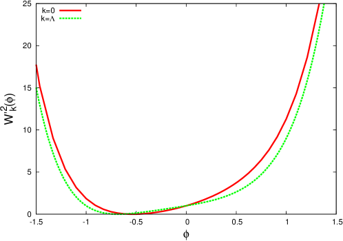
Figure 1: The scalar potential $V=\frac{1}{2}W^{\prime}(\phi)^{2}$ before and after the flow

VI.4 System of two coupled field dependent flow equations

As an example for a system of two coupled flow equations we consider supersymmetric quantum mechanics with field dependent wave function renormalization.

As in the previous section, the flow equations with a field dependent wave function renormalization are discussed in Synatschke:2008pv . They read

$$\partial_{k}W^{\prime}_{k}(\phi)= -W^{\prime\prime\prime}_{k}\frac{\mathcal{N}}{4\mathcal{D}^{2}}$$ (21)

$$Z_{k}(\phi)\partial_{k}Z_{k}(\phi)= \left(\frac{4Z^{\prime}_{k}(\phi)W^{\prime\prime\prime}_{k}(\phi)}{\mathcal{D}}-\big{(}Z_{k}^{\prime}(\phi)Z_{k}(\phi)\big{)}^{\prime}-\frac{3Z_{k}(\phi)^{2}W^{\prime\prime\prime}_{k}(\phi)^{2}}{4\mathcal{D}^{2}}\right)\frac{\mathcal{N}}{4{\mathcal{D}}^{2}}\,,$$

where we have introduced the abbreviations

$$\mathcal{N}=(1+k\partial_{k})Z_{k}(\phi)^{2}\quad\text{and}\quad\mathcal{D}=W^{\prime\prime}(\phi)+kZ_{k}(\phi)^{2}\,.$$ (22)

The python script to solve these equations is given in Listing 5. The solutions are shown in Fig 2. This picture was created with n_steps=40.

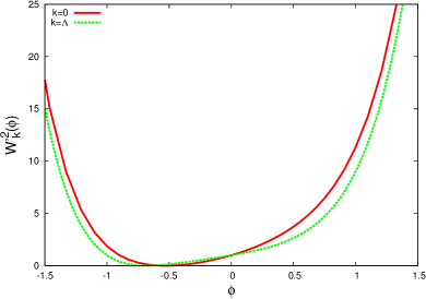
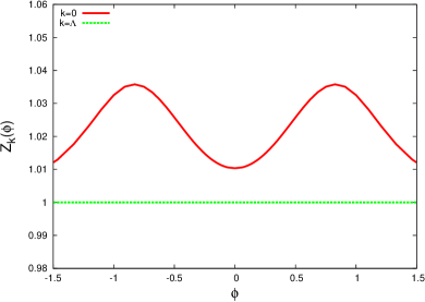
Figure 2: left panel: Scalar potential $V=\frac{1}{2}W^{\prime 2}$, right panel: field dependent wave function

Listing 5: An example for a system of two coupled differential equations

⬇

# SUSY_QM_wavefunction.py

import FlowPy

SUSY_eqns="""

d/dk V(k,phi)=-V’’(k,phi)*(Z(k,phi)^2+2*k*Z(k,phi)*d/dk Z(k,phi))

/4/(V’(k,phi)+k*Z(k,phi)^2)^2;

d/dk Z(k,phi)=(Z(k,phi)+2*k*d/dk Z(k,phi))

/4/(V’(k,phi)+k*Z(k,phi)^2)^2

*(4*Z’(k,phi)*V’’(k,phi)/(V’(k,phi)+k*Z(k,phi)^2)

-Z’’(k,phi)*Z(k,phi)-Z’(k,phi)*Z’(k,phi)

-3*Z(k,phi)^2*V’’(k,phi)^2/4/(V’(k,phi)

+k*Z(k,phi)^2)^2);

FLOWSTART V(k,phi) = e+m*phi+g*phi^2+a*phi^3;

FLOWSTART Z(k,phi) = 1;

#==== Parameters ====

e=1.0;

m=1.0;

g=0.1;

a=1.0;

"""

#change n_start and n_end to change the phi_range

n_start=-2

n_end=2

n_steps=10 #increase this variable to improve the resolution

xs=FlowPy.linrange(n_start,n_end,n_steps)

logger=FlowPy.make_flow_logger(filename="SUSY_QM_wavefunction.flow")

fp=FlowPy.flowproblem("flowpy_SUSY_QM_wavefunction",

xs=xs,

equations=SUSY_eqns,

log_state=logger,

decide_iterate=FlowPy.make_lhs_iterator(loops=0),

verbose=2,

)

fp.flow()

VI.5 Momentum-dependent flow equations

FlowPy can also solve flow equations with full momentum dependence. In this example we calculate the momentum dependent wave-function renormalization for the supersymmetric $N=2$ Wess-Zumino Model in two dimensions. This model is thoroughly discussed in Synatschke:2010jn where the flow equation is derived. The flow equation read

$$\partial_{k}Z_{k}^{2}(p)=-16g^{2}\int\frac{d^{2}q}{4\pi^{2}}\frac{kZ^{2}_{k}\left(q\right)+{m}}{N({\bm{q}})^{2}N({\bm{p}}-{\bm{q}})}Z^{2}_{k}\left(q\right)Z^{2}_{k}\left(\left|{\bm{p}}-{\bm{q}}\right|\right)\partial_{k}\left(kZ_{k}^{2}\left(q\right)\right),$$ (23)

where we have introduced the abbreviation

$$N({\bm{q}})=\left(q^{2}Z^{4}_{k}\left(q\right)+(kZ^{2}_{k}\left(q\right)+{m})^{2}\right).$$ (24)

${\bm{q}}$ and ${\bm{p}}$ denote two dimensional vectors, whereas $q=\left|{\bm{q}}\right|$ and $p=\left|{\bm{p}}\right|$ respectively.

A python script to solve this equation with $m=1$ and $g=0.3$ is given in Listing 6. Note that due to the complex structure of the flow equation this script takes a long time to calculate the wave function even with a very low resolution of five sampling points. The result is shown in Fig. 3. The calculation was done with n_steps=30.

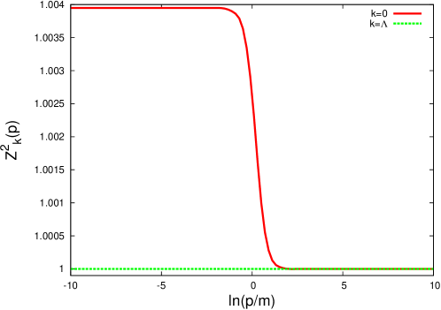
Figure 3: Momentum dependent wave function renormalization

Listing 6: An example for a momentum dependent wave function

⬇

# momentum_dependent_wavefunction.py

import FlowPy

import math

wavefunction_eqns="""

d/dk Z(k,p) =

integral[d phi from -pi to pi,

d q from 0 to k]

(-16*g^2)/4/pi^2*(k*Z(k,q)+m)*Z(k,q)*Z(k,Cminus(p,q,phi))

*(1+k*d/dk Z(k,q))/(q*q*Z(k,q)*Z(k,q)+(k*Z(k,q)+m)*(k*Z(k,q)+m))

/(Cminus(p,q,phi)*Cminus(p,q,phi)*Z(k,Cminus(p,q,phi))

*Z(k,Cminus(p,q,phi))+(k*Z(k,Cminus(p,q,phi))+m)

*(k*Z(k,Cminus(p,q,phi))+m))

/(q*q*Z(k,q)*Z(k,q)+(k*Z(k,q)+m)*(k*Z(k,q)+m))^2;

FLOWSTART Z(k,p) =1;

# === Helper functions ===

Cminus(p1,p2,alpha) = p1^2+p2^2-2*p1*p2*cos(alpha);

# === Parameters ===

m = 1.0;

g=0.3;

pi=3.141592653589793;

"""

#change n_start and n_end to change the p_range

n_start=-20

n_end=10

n_steps=5 #increase this number of sampling points to improve the resolution

# logarithmic-equidistant distribution of the momentum:

qs_log=FlowPy.linrange(n_start,n_end,n_steps)

qs=[-math.exp(q) for q in qs_log]+[0.0]+[math.exp(q) for q in qs_log]

# specifing the logfile:

logger=FlowPy.make_flow_logger(filename="momentum_dependent_wavefunction.flow")

# solving the flow equation:

fp=FlowPy.flowproblem("flowpy_wavefunction",

xs=qs,

equations=wavefunction_eqns,

log_state=logger,

decide_iterate=FlowPy.make_lhs_iterator(loops=0),

verbose=2)

fp.flow()

VI.6 Parametric Example

In some situations, one would want to perform a number of renormalization group flow calculations that differ only in the choice of some parameters. While this can be achieved in a reasonably straightforward way with FlowPy via Python scripting, the FlowPy package contains a few extra definitions to make this process more convenient for the user, which are explained by means of an example in Listing 7.

Listing 7: Example for a flow equation with two parameters

⬇

# parametric.py

from FlowPy import flowproblem, flowparams, make_lhs_iterator,\

grange, make_flow_logger

runs_todo=[flowparams(mu=val_mu,T=val_T)

for val_mu in [1.0,1.5,2.0,2.5]

for val_T in [0.1,0.2,0.5,1.0]]

xs=[float(n) for n in range(11)]

for params in runs_todo:

f=flowproblem("mu_T",

xs=xs,

equations="""

d/dk F(k,p) = -T;

FLOWSTART F(k,p) = mu;

"""+params.defs(),

ks=grange(110,10,5),

decide_iterate=make_lhs_iterator(loops=0),

log_state=make_flow_logger(\

params.subs_short("FLOW__mu=${mu}_T=${T}__.flow")),

verbose=2)

f.flow()

The key concept here is the flowparams “FlowPy parameters” object. This represents a collection of parameter choices that can easily be mapped to strings in various contexts, e. g. to generate systematic output filenames. A flowparams object is created by specifying explicitly all “parameter name = numerical value” associations in a function call of the form

⬇

params = flowparams(mu=1.5, alpha=3.0, T=0.5)

A potentially relevant limitation is that special keywords in the Python programming language (such as e. g. def, raise, lambda, else, etc.) cannot be chosen as parameter names. (There is a way to avoid this problem in Python by using a different function call form, should this really turn out to be a problem.)

If params is a FlowPy parameter object, e. g. defined as in the example in Listings 7, then params.defs() will produce a string containing valid FlowPy constant definitions that introduce these parameters. One would typically want to append this to the (parameter-dependent) flow equation definitions by using Python “string addition” as shown in the example. Another useful snippet is params.subs_short(pattern) which will regard pattern as a template string on which parameter substitution has to be performed according to the rules of Python’s string.Template class, i.e. ${xyz} will be substituted by the pretty-printed numerical value of the parameter xyz. (Detailed rules can be found in the Python documentation of the string.Template mechanism.) One may want to use this to automatically generate filenames, as shown in the example.

A very useful Python feature one might want to employ in such situations is special syntax available to define lists from cartesian products. In Python, one can e. g. write

⬇

[(x,y) for x in range(1,5) for y in range(1,x)]

to obtain the list

⬇

[(2, 1), (3, 1), (3, 2), (4, 1), (4, 2), (4, 3)]

This syntax, which is an adoption of a very similar feature that probably was first made popular through the Haskell programming language, can be used to concisely specify fairly complex constructions, such as

⬇

from fractions import gcd

[(x,y,x*y) for x in range(5) for y in range(5) if gcd(x,y)==1]

which gives the list

⬇

[(0, 1, 0),

(1, 0, 0),

(1, 1, 1),

(1, 2, 2),

(1, 3, 3),

(1, 4, 4),

(2, 1, 2),

(2, 3, 6),

(3, 1, 3),

(3, 2, 6),

(3, 4, 12),

(4, 1, 4),

(4, 3, 12)]

Users of FlowPy might find the basic form of this construct useful to define cartesian products of parameter choices, as in the example provided in this section.

Evidently, if the approach shown here is used to perform $N$ different numerical renormalization group flow calculations, then $N$ different machine code files will be produced automatically by FlowPy and loaded into Python. Although this process could be improved conceptually, this would presumably be only worthwhile for $N\gg 100$. This is unlikely to be relevant for typical applications, as problems of typical complexity are expected to be partitioned into collections of $N<100$ before being submitted to a computing cluster anyway. When performing multiple FlowPy calculations on a cluster, one should ensure that each cluster job chooses a different name when defining a flowproblem. Otherwise, this may result in accidental unintended sharing of the directory used to produce machine code, and some calculations may fail or, even worse, end up using a wrong set of parameters and equations. Typically, an unique job ID will be taken from the program’s argument list, from environment variables, or generated semi-randomly using the time and process ID. Python makes this information available via the sys.argv variable containing program arguments (the sys module has to be imported first), the os.getenv() function that behaves like the corresponding C library function, the time.time() and related functions, and the random module.

VII Current limitations

In its present form, the FlowPy package has a number of limitations. None of these are actually fundamental – they all could be overcome with some dedicated effort on the side of the FlowPy authors. Concerning the question how relevant these are, and where to focus further development effort on, the authors seek input from the renormalization group flow community.

Present limitations are:

• FlowPy assumes every flow function to depend on precisely one extra parameter beyond the scale parameter $k$.

• The right-hand side of flow functions may involve zero to two integrals, and the integration boundaries may only depend on left-hand side parameters, i. e. the inner integration boundary cannot depend on the value of the outer integration parameter. Also, term notation presently requires integral specifications to follow the equals sign directly, i. e. all extra factors must be pulled under the integral. Expressions such as $C\int_{\alpha=-\pi}^{\pi}d\alpha\,f(\alpha)$ (with $C$ a numerical constant) hence must be re-written as $\int_{\alpha=-\pi}^{\pi}d\alpha\,Cf(\alpha)$.

• Currently boundary conditions in the $x$ direction are fixed to the classical values of the effective potential. However, more flexible boundary conditions that can be specified by the user might be more appropriate for some problems.

• The range of special functions made available to the user so far is fairly limited.

• Error reporting could be improved to make it easier to find typos in the specification of the flow equations.

• FlowPy suffers from some minor bugs in the default parser definitions inherited from python-simpleparse. In particular, a number such as ‘5e-3’ is not a valid constant – this must be given as ‘5.0e-3’ instead.

• This version of FlowPy does not support parallelization. However, re-introducing MPI support is planned.

• There are many opportunities to make FlowPy more efficient by improving its internal design. This, however, will require substantial low level changes.

VIII Outlook

In this paper we present the numerical toolbox FlowPy which is able to solve many typical partial differential equations encountered in studies of the functional renormalization group. We hope that it will prove to be useful in the application of functional renormalization group techniques and that it will facilitate these studies in providing a powerful numerical tool to solve the differential equations.

We plan to include MPI support in the next version of FlowPy. Additionally it is planned to make the boundary conditions in the field variable more flexible such that it will be possible to use e. g. the first loop approximation. Also there is a lot of room for improvement in the performance of the parser. Here we present the first version of FlowPy and we have planned to release updates in the future. The intention of this paper is to make FlowPy available to a wider audience. Thus we are grateful for suggestions how to improve FlowPy.

IX Acknowledgments

The authors would like to thank J. Braun, H. Gies and A. Wipf for helpful discussions and valuable comments on the manuscript. Also, the authors would like to thank Max Albert for helping with the effort to port FlowPy to the Mac OS X platform. Part of this work was supported by the German Science Foundation (DFG) under GRK 1523 and the Studienstiftung des deutschen Volkes e. V.

References

- (1) Daniel F. Litim and Jan M. Pawlowski. On gauge invariant Wilsonian flows, 1998. hep-th/9901063.
- (2) K. Aoki. Introduction to the nonperturbative renormalization group and its recent applications. Int. J. Mod. Phys., B14:1249–1326, 2000.
- (3) Jurgen Berges, Nikolaos Tetradis, and Christof Wetterich. Non-perturbative renormalization flow in quantum field theory and statistical physics. Phys. Rept., 363:223–386, 2002. hep-ph/0005122.
- (4) Janos Polonyi. Lectures on the functional renormalization group method. Central Eur. J. Phys., 1:1–71, 2003. hep-th/0110026
- (5) Jan M. Pawlowski. Aspects of the functional renormalisation group. Annals Phys., 322:2831–2915, 2007. hep-th/0512261.
- (6) Holger Gies. Introduction to the functional RG and applications to gauge theories, 2006. hep-ph/0611146.
- (7) Hidenori Sonoda. The Exact Renormalization Group – renormalization theory revisited –, 2007. arXiv:0710.1662 [hep-th].
- (8) Bertrand Delamotte. An introduction to the nonperturbative renormalization group. 2007. cond-mat/0702365.
- (9) C. Bagnuls and C. Bervillier, Exact renormalization group equations. An Introductory review. Phys. Rept. 348, 91 (2001). hep-th/0002034.
- (10) Franziska Synatschke, Holger Gies, and Andreas Wipf. Phase Diagram and Fixed-Point Structure of two dimensional N=1 Wess-Zumino Models. Phys. Rev., D80:085007, 2009. arXiv:0907.4229 [hep-th].
- (11) Franziska Synatschke, Jens Braun, and Andreas Wipf. N=1 Wess Zumino Model in d=3 at zero and finite temperature. Phys. Rev., D81:125001, 2010. arXiv:1001.2399 [hep-th].
- (12) Jan M. Pawlowski. The QCD phase diagram: Results and challenges. AIP Conf.Proc., 1343:75–80, 2011. arXiv:1012.5075 [hep-ph].
- (13) Jens Braun. Fermion Interactions and Universal Behavior in Strongly Interacting Theories. J. Phys. G G 39 (2012) 033001 2011. arXiv:1108.4449 [hep-ph].
- (14) Christof Wetterich. Exact evolution equation for the effective potential. Phys. Lett., B301:90–94, 1993.
- (15) Markus Q. Huber and Jens Braun. Algorithmic derivation of functional renormalization group equations and Dyson-Schwinger equations. 2011. arXiv:1112.6173 [hep-th].
- (16) Franziska Synatschke, Georg Bergner, Holger Gies, and Andreas Wipf. Flow Equation for Supersymmetric Quantum Mechanics. JHEP, 03:028, 2009. arXiv:0809.4396 [hep-th].
- (17) Ulrich Ellwanger, Manfred Hirsch, and Axel Weber. Flow equations for the relevant part of the pure Yang- Mills action. Z. Phys., C69:687–698, 1996. hep-th/9506019.
- (18) Jan M. Pawlowski, Daniel F. Litim, Sergei Nedelko, and Lorenz von Smekal. Infrared behaviour and fixed points in Landau gauge QCD. Phys. Rev. Lett., 93:152002, 2004. hep-th/0312324.
- (19) Christian S. Fischer and Holger Gies. Renormalization flow of Yang-Mills propagators. JHEP, 10:048, 2004. hep-ph/0408089.
- (20) Christian S. Fischer, Axel Maas and Jan M. Pawlowski. On the infrared behavior of Landau gauge Yang-Mills theory. Annals Phys. 324, 2408 (2009). arXiv:0810.1987 [hep-ph].
- (21) Jean-Paul Blaizot, Ramon Mendez-Galain, and Nicolas Wschebor. Non perturbative renormalization group and momentum dependence of n-point functions. II. Phys. Rev., E74:051117, 2006. hep-th/0603163.
- (22) Jean-Paul Blaizot, Ramon Mendez-Galain, and Nicolas Wschebor. Non perturbative renormalisation group and momentum dependence of n-point functions. I. Phys. Rev., E74:051116, 2006. hep-th/0512317.
- (23) J. P. Blaizot, Ramon Mendez Galain, and Nicolas Wschebor. A new method to solve the non perturbative renormalization group equations. Phys. Lett., B632:571–578, 2006. hep-th/0503103.
- (24) F. Benitez et al. Solutions of renormalization group flow equations with full momentum dependence. Phys. Rev., E80:030103, 2009. arXiv:0901.0128 [cond-mat.stat-mech].
- (25) S. Diehl, H. C. Krahl, and M. Scherer. Three-Body Scattering from Nonperturbative Flow Equations. Phys. Rev., C78:034001, 2008. arXiv:0712.2846 [cond-mat.stat-mech].
- (26) Leonard Fister and Jan M. Pawlowski. Yang-Mills correlation functions at finite temperature. 2011. arXiv:1112.5440 [hep-ph]
- (27) http://www.netlib.org/odepack/.
- (28) http://www.netlib.org/fitpack/.
- (29) http://www.netlib.org/quadpack/.
- (30) http://www.scipy.org/.
- (31) Franziska Synatschke, Thomas Fischbacher, and Georg Bergner. The two dimensional N=(2,2) Wess-Zumino Model in the Functional Renormalization Group Approach. 2010. arXiv:1006.1823 [hep-th].
- (32) Markus Q. Huber and Mario Mitter. CrasyDSE: A framework for solving Dyson-Schwinger equations. 2011. arXiv:1112.5622 [hep-th]