Analysis of a data matrix and a graph: Metagenomic data and the phylogenetic tree

Abstract

In biological experiments researchers often have information in the form of a graph that supplements observed numerical data. Incorporating the knowledge contained in these graphs into an analysis of the numerical data is an important and nontrivial task. We look at the example of metagenomic data—data from a genomic survey of the abundance of different species of bacteria in a sample. Here, the graph of interest is a phylogenetic tree depicting the interspecies relationships among the bacteria species. We illustrate that analysis of the data in a nonstandard inner-product space effectively uses this additional graphical information and produces more meaningful results.

t1Supported in part by a NSF Post-doctoral Fellowship in Biological Informatics and by NSF Grant 02-41246.

1 Introduction

Relationships among either observations or variables are often conveniently summarized by a graph. Incorporating this outside information into the analysis of numerical data is of increasing interest, particularly in biology where many known properties of genes and proteins are described by complicated networks. A common situation is to have numerical data from an experiment which is of primary interest and also additional knowledge in the form of a graph relating our observations or variables from the experiment. We would like to incorporate the information in the graph with our analysis of the experimental data. By including the graphical information directly in our analysis, we constrain the space of possible solutions to those that are relevant from the point of view of the known information.

The specific type of graph which we consider here is a phylogenetic tree. A phylogenetic tree is a ubiquitous graph in biology that describes the evolutionary relationship between a set of species. We are motivated to consider this graph by our work with Eckburg et al. (2005) analyzing differences in bacterial composition based on a genomic inventory of different samples. Such “metagenomic” studies are a popular technique for measuring bacterial content. As we argue below, using the phylogenetic information regarding the discovered bacteria is key in creating a meaningful analysis—particularly because of the small sample size relative to the number of bacteria found.

There are numerous different strategies for using graphical information, such as Bayesian networks and differential equation modeling; they require varying degrees of specificity in the graphical information. We focus here on a technique that is simple to implement and uses the graph to define a nonstandard inner-product space in $\mathbb{R}^{p}$ to perform the analysis of the numerical data.

The layout of the paper is as follows. First we will introduce the motivating example of bacterial composition in more detail and will return to the example at the end to demonstrate the techniques on the bacterial data. We review how PCA can be succinctly reformulated for nonstandard inner-products and its development for ecological studies of species abundance, a reformulation we will call generalized PCA (gPCA). The rest of the paper delves further into the implications of incorporating outside graphical information through the use of such a metric space. In particular, we give an appropriate metric for a phylogenetic tree and evaluate the implications of that choice in the final data analysis. Throughout, we focus on the example of the phylogenetic tree and metagenomic data to illustrate the concepts. However, the same basic approach can be useful in including nonstandard forms of knowledge—other types of graphical information in particular.

Notation. In all that follows, we will use boldface type to indicate vectors and matrices and parenthetical subscripts to indicate elements of vectors and matrices. Therefore, the $j$th component of a vector ${\mathbf{x}_{{i}}}$ will be given as ${\mathbf{x}_{{i}{(j)}}}$ and the $i,j$ element of a matrix ${\mathbf{A}}$ will be given as ${\mathbf{A}_{(ij)}}$.

2 Motivating example

In Eckburg et al. (2005) the broad goal was to describe the kinds of bacteria found in the intestinal tract and compare the bacterial communities found in different people. To that end, each of the three patients in the study had biopsies taken at six locations in his/her colon in addition to providing a stool sample. Each of these seven samples (per patient) was then subjected to genomic techniques to try to quantify the different types of bacteria as well as their abundance.

Traditional techniques for identifying bacteria require growing the bacteria in a culture and then classifying the bacteria as a species based on any observable characteristics as well as the nutrients needed for it to grow. This gives only limited ability to assess the presence of different types of bacteria. The increased ease of DNA sequencing has led researchers to classify bacteria by genomic information (“metagenomics”). We focus here on the results of sequencing a specific gene (16S rDNA) found in bacteria. A random selection of all the copies of the gene present in the sample are sequenced. Ideally, each version of the gene could be uniquely identified as coming from a specific bacteria and the abundance of the different gene versions would give an estimate of the abundance of each bacteria. In reality, we do not have a direct link between a gene version and its originating bacteria, but only an estimate of it, as we explain more fully below.

Bacteria species also share an evolutionary history which might affect their biological role in the sample. We summarize the evolutionary relationship by a phylogenetic tree that describes the evolutionary history of the bacterial species. We visualize both the phylogenetic tree relating the bacterial species and their numerical abundance in Figure 1. There is a great deal of sparsity in the data; many species are present in low numbers and in only a few samples. At the same time, there are some highly abundant species found at high levels in most samples. From this visual inspection, we can also see the importance of jointly considering both aspects of the data—entire regions of the phylogenetic tree appear dissimilar between the patients, such as the Bacteriodetes phylum (colored shades of blue) where patient A has much less abundance across all of his/her samples than the other two patients.

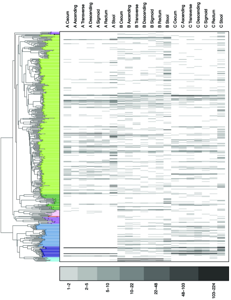
Figure 1: Depiction of the abundance matrix from Eckburg et al. (2005). Columns indicate samples, grouped by patient, and rows correspond to different phylotypes. The grey scale indicates the level of abundance on a log scale (see legend for conversion to original abundances). The colors on the phylogenetic tree indicate phylum, as in Eckburg et al. (2005), but with a different choice of colors: blue—Bacteriodetes, green—Firmicutes, purple—various Proteobacteria, pink—Verrucomicrobia. We additionally colored two portions of the Bacteriodetes phylum (blue) separately: roughly identifiable as Prevotallae and B. vulgatus, they are colored lightest blue and darkest blue, respectively. Also, we colored the Firmicutes (green) with two different shades for B. Mollicutes and Clostridia (dark green and light green, respectively).

Given the large number of species (395) as compared to the number of samples (21), we could reorder the species and find other sets of species that are also very different across the patients. However, the clusters defined by the phylogenetic tree provide biological information regarding the relationships among the species that is separate from the numerical abundances. Patterns of sparsity or differences among the patients following the clusters in the tree are generally of greater interest than an arbitrary grouping since there is known biological meaning to the groupings. The additional information found by using the phylogenetic similarities can serve as a check on the kind of relationships among the species that we are interested in. This will be particularly important since we have so many more species than samples. Focusing the analysis to follow the structure of the tree will allow for more meaningful results.

This study was exploratory. It was the first sequence-based analysis of the bacterial composition of the colon that compared between individuals and/or locations of the sample (many genomic experiments of this type either sampled only one patient or pooled patients together). The list of phylotypes found and their relationship to known bacterial taxa was biologically informative. In addition to creating an inventory, the goals of the experiment were to better describe the bacteria communities and their differences along the intestinal tract or between patients. With the small sample size, the analysis cannot extrapolate to the population in general but can only focus on describing the patients observed.

2.1 Effect of imperfect species definition

In practice, we cannot identify a bacterial species from the DNA sequence. Instead the sequences are themselves used to define the species, based on the sequence similarity of different copies—for example, the rule in Eckburg et al. (2005) for grouping sequences into one “species” required all pairs in the group to have a minimum of 99% sequence similarity. For this reason, the term “phylotype” is used instead of species to indicate that these are merely proxies for the true species distinctions. A phylogenetic tree for the phylotypes was built using maximum likelihood estimation of the tree [Felsenstein (1981)]. Specifically, the tree was built using a representative instance of the 16S rDNA sequence from each phylotype, generally a consensus sequence of those sequences classified into that phylotype.

The possible effect of using an arbitrary cutoff for defining phylotypes is seen in Figure 1, where the length of the tree branch reflects the similarity between the species. Some phylotypes clearly form tight bunches of very similar phylotypes, particularly in the Clostridia family of the Firmicutes phylum (light green). If we had changed the cutoff for defining phylotypes, we could imagine these groups collapsing into a few distinct phylotypes. Therefore, we need to be careful to have an analysis that is robust to such small changes and does not count each phylotype as equally important.

The relationship between DNA sequences can be summarized in different ways, such as its similarity to other sequences, the phylotype to which it has been assigned, or its location in a phylogenetic tree built between different sequences. The analysis discussed in detail here will reduce the sequence data to the phylotype-level, ignoring the individual sequence data: each of the $N=11\mbox{,}831$ observations (or sequenced strands of DNA) belongs to one of $S=395$ phylotypes (or species) and one of the ${L}=21$ locations.

3 Incorporation of additional information via inner-products

For observed data ${\mathbf{x}_{{i}}}\in\mathbb{R}^{{p}}$ we propose to use nonstandard inner-products or metrics in analyzing the data. We argue that this is a simple way to include complicated outside information, such as graphical information, in the analysis of high-dimensional data.

By nonstandard inner-products, we specifically mean an inner-product between two observations $i$ and $j$ given by $\langle{\mathbf{x}_{{i}}},{\mathbf{x}_{{j}}}\rangle_{{\mathbf{Q}}}={\mathbf{x}_{{i}}}^{T}{\mathbf{Q}}{\mathbf{y}_{{j}}}$. Since ${\mathbf{Q}}$ also defines a metric based on $\|{\mathbf{x}_{{i}}}-{\mathbf{x}_{{j}}}\|_{{\mathbf{Q}}}$, we may at times refer to ${\mathbf{Q}}$ as a metric. For any inner-product $\langle\cdot,\cdot\rangle$ and a fixed set of $n$ vectors ${\mathbf{x}_{{i}}}$, there exists a matrix ${\mathbf{Q}}$ so that $\langle{\mathbf{x}_{{i}}},{\mathbf{x}_{{j}}}\rangle={\mathbf{x}_{{i}}}^{T}{\mathbf{Q}}{\mathbf{x}_{{j}}}$, so this is a quite general definition. A common example of such an inner-product is the Mahalanobis distance, where ${\mathbf{Q}}$ is chosen as the inverse covariance matrix of the observed random vectors [see Maesschalck, Jouan-Rimbaud and Massart (2000)]. In this case, the choice of ${\mathbf{Q}}={\mathbf{{\mathbf{\bolds{\Psi}}}}}^{-1}$, where ${\mathbf{{\mathbf{\bolds{\Psi}}}}}$ is the covariance matrix of the observed variables, removes the correlation among the variables, also known as “sphering” the data. This is the most common choice of a nontrivial ${\mathbf{Q}}_{{p}}$ and is used, for example, in discriminant analysis for classification problems.

The choice of an appropriate metric ${\mathbf{Q}}$, however, can also be a method for including outside information. In particular, assume that the additional information, such as the phylogenetic tree, is such that one can model the covariance structure ${\bolds{\Sigma}}$ for the variables that this information would imply. The resulting covariance matrix, $\bolds{\Sigma}$, is not the covariance for the observed variables in our data—which is the result of a much more complicated relationship between the graph and the data—but rather what would be expected if the data was completely created by this outside process. In order to evaluate the data so as to give priority to relationships in the phylogenetic tree, we propose using the metric ${\mathbf{Q}}_{{p}}=\bolds{\Sigma}$ for the variable space. Performed in this space, the analysis focuses on the aspects of the data variables most congruent with the $\bolds{\Sigma}$.

Because most multivariate techniques are based on inner-products, they are easily generalized to a more general inner-product space. We will focus on PCA using ${\mathbf{Q}}$, a technique known as generalized PCA (gPCA) or the duality principle [Escoufier (1987); Holmes (2008); Dray and Dufour (2007)]; Jolliffe (2002) gives a more in depth overview of gPCA, connecting gPCA with other techniques. We give a short review of gPCA before we discuss more fully the interpretation of this strategy. Other multivariate methods have been similarly extended and would be also relevant for incorporation of outside information.

3.1 Generalized PCA

Quite generally, gPCA is an ordination procedure, that is, each observed data point ${\mathbf{x}}\in\mathbb{R}^{{p}}$ is transformed to new, lower-dimensional data coordinates given by ${\mathbf{\hat{x}}}\in\mathbb{R}^{k}$ which is a linear transformation of the original coordinates: ${\mathbf{\hat{x}}}={\mathbf{Z}}^{T}{\mathbf{x}}$ for some matrix ${\mathbf{Z}}\in\mathbb{R}^{{p}\times k}.$ Most multivariate techniques are ordination procedures, common examples being PCA, Canonical Correlation Analysis and Correspondence Analysis. The differences lie in the choice of the linear transformation (${\mathbf{Z}}$), which is chosen based on the desired properties of the new, lower-dimensional vector ${\mathbf{\hat{x}}}$. The most familiar example is standard PCA which seeks successive vectors ${\mathbf{a}_{{j}}}\in\mathbb{R}^{p}$ so that the resulting $j$th coordinate, ${\mathbf{\hat{x}}_{{}{(j)}}}=\langle{\mathbf{x}},{\mathbf{a}_{{j}}}\rangle,$ has the largest variance, subject to being independent of previous coordinates ${\mathbf{x}_{{}{(1)}}},\ldots,{\mathbf{x}_{{}{(j-1)}}}$; the final transformation matrix is ${\mathbf{Z}}={\mathbf{A}}_{k}=({\mathbf{a}_{{1}}}\cdots{\mathbf{a}_{{k}}})$.

The ordination procedure of generalized PCA (gPCA) is a generalization of PCA in that it assumes an alternative inner-product for the data vectors ${\mathbf{x}}$. We assume an observed random variable ${\mathbf{x}}$ lies in $\mathbb{R}^{p}$ with a known inner-product defined by ${\mathbf{Q}}_{{p}}\in\mathbb{R}^{{p}\times{p}}$. Then in analogy with standard principal components, gPCA can be developed from the perspective of finding the vector ${\mathbf{a}}$ that maximizes the population quantity, $\operatorname{var}(\langle{\mathbf{a}},{\mathbf{x}}\rangle_{{\mathbf{Q}}_{{p}}}),$ with ${\mathbf{a}}$ constrained to have unit ${\mathbf{Q}}_{{p}}$-norm and successive ${\mathbf{a}_{{j}}}$ constrained to be ${\mathbf{Q}}_{{p}}$-orthogonal to the preceding ${\mathbf{a}_{{j}}}$,

$$\|{\mathbf{a}_{{j}}}\|_{{\mathbf{Q}}_{{p}}}=1\quad\mbox{and}\quad{\mathbf{A}}_{k}^{T}{\mathbf{Q}}_{{p}}{\mathbf{A}}_{k}={\mathbf{I}}_{k},$$

where, again, ${\mathbf{A}}_{k}\in\mathbb{R}^{{p}\times k}$ is the matrix with columns ${\mathbf{a}_{{j}}}$. The new coordinates for ${\mathbf{x}}$ are then given by ${\mathbf{\hat{x}}}={\mathbf{A}}_{k}^{T}{\mathbf{Q}}_{{p}}{\mathbf{x}}$ (so ${\mathbf{Z}}={\mathbf{A}}_{k}^{T}{\mathbf{Q}}_{{p}}$ in the notation given above). As in PCA, the ${\mathbf{a}_{{j}}}$ will be eigenvectors, but now of the matrix ${\mathbf{\bolds{\Psi}}}{\mathbf{Q}}_{{p}}$ where ${\mathbf{\bolds{\Psi}}}$ is the covariance matrix of ${\mathbf{x}}$. The matrix ${\mathbf{\bolds{\Psi}}}{\mathbf{Q}}_{{p}}$ is not symmetric, but because ${\mathbf{Q}}_{{p}}$ is full rank, this is a well defined, positive definite generalized eigenequation, and the eigenvectors of ${\mathbf{\bolds{\Psi}}}{\mathbf{Q}}_{{p}}$ can be chosen to be a ${\mathbf{Q}}_{{p}}$-orthogonal set of vectors [see Golub and van Loan (1996)].

Just as in PCA, there are multiple developments that result in the same ordination procedure. For example, gPCA provides the best $k$-dimensional approximation to the inter-point similarities when the similarities are calculated in the appropriate metric space. In particular, we could note that if distances between observation $i$ and $j$ are given by

$$d(i,j)=({\mathbf{x}_{{i}}}-{\mathbf{x}_{{j}}})^{T}{\mathbf{Q}}_{{p}}({\mathbf{x}_{{i}}}-{\mathbf{x}_{{j}}}),$$

then gPCA is equivalent to Multidimensional Scaling (MDS) of the ${n}$ observations based on these distances. Similarly, for any ${\mathbf{Q}}_{{p}}$, there exists a (nonunique) matrix ${\mathbf{C}}$ so that ${\mathbf{Q}}_{{p}}={\mathbf{C}}{\mathbf{C}}^{T}$, which means gPCA of ${\mathbf{x}}$ based on ${\mathbf{Q}}_{{p}}$ is equivalent to first transforming the vector ${\mathbf{x}}$ by ${\mathbf{C}}$ and then performing PCA on the resulting vector ${\mathbf{C}}^{T}{\mathbf{x}}$.

Metric for the columns. As an analysis of a ${n}\times{p}$ data matrix ${\mathbf{X}}$, the above presentation only considered a metric for the space of row vectors (observations) of ${\mathbf{X}}$. There can also be a relevant metric for comparison of the variables, a simple example being when there are weights assigned to the observations. Generalized PCA goes beyond the description given so far and allows also for a metric ${\mathbf{Q}}_{{n}}\in\mathbb{R}^{{n}\times{n}}$ for the space of the column vectors of ${\mathbf{X}}$. These combinations of choices are generally abbreviated as the triplet $({\mathbf{X}},{\mathbf{Q}}_{{p}},{\mathbf{Q}}_{{n}})$ [see Escoufier (1987) for a more general explanation of the role of two separate metrics when viewing ${\mathbf{X}}$ as an operator simultaneously in $\mathbb{R}^{{p}}$ and $\mathbb{R}^{{n}}$]. We note that in many cases either ${\mathbf{Q}}_{{n}}$ or ${\mathbf{Q}}_{{p}}$ are chosen to be diagonal, in which case they simplify to weights on the observations or variables, respectively.

Returning to the population development above, the inclusion of a metric for the columns of ${\mathbf{X}}$ is incorporated in the estimation of ${\mathbf{\bolds{\Psi}}}.$ In order to maximize the quantity $\operatorname{var}(\langle{\mathbf{a}},{\mathbf{x}}\rangle_{{\mathbf{Q}}_{{p}}})$, we must estimate ${\mathbf{\bolds{\Psi}}}$ from our data matrix ${\mathbf{X}}$; we include the metric ${\mathbf{Q}}_{{n}}$ for the columns in our estimate so that ${\mathbf{\widehat{{\mathbf{\bolds{\Psi}}}}}}={\mathbf{X}}^{T}{\mathbf{Q}}_{{n}}{\mathbf{X}}$. Then our estimates of ${\mathbf{a}_{{j}}}$ are given by the eigenvectors of ${\mathbf{X}}^{T}{\mathbf{Q}}_{{n}}{\mathbf{X}}{\mathbf{Q}}_{{p}}$. A geometric development that includes the metric ${\mathbf{Q}}_{{n}}$ for the columns shows that gPCA best preserves the total inner-point similarities of the data matrix ${\mathbf{X}}$ when using a measure of inner-point similarities incorporating the row and column matrix known as the inertia (see Appendix C). In addition to the geometric view of gPCA, Jolliffe (2002) notes that gPCA with ${\mathbf{Q}}_{{n}}$ a diagonal matrix provides the maximum likelihood estimates of the fixed effects version of a factor model,

$${\mathbf{x}}={\mathbf{A}}{\mathbf{z}}+{\mathbf{\bolds\varepsilon}},$$

where ${\mathbf{\bolds\varepsilon}}\sim N({\mathbf{0}},\sigma^{2}{\mathbf{Q}}_{{n}}^{-1}{\mathbf{Q}}_{{p}}^{-1}).$

Connection between analysis of the rows and columns. In some data settings either the rows or the columns can be meaningfully considered as the observations, such as analysis of large contingency tables that are our motivating example. Furthermore, the importance of the different variables in describing a low-dimensional representation of the observations is a common part of PCA. A gPCA of the columns of ${\mathbf{X}}$, also reduced to $k$ dimensions, is technically the gPCA of triplet $({\mathbf{Y}}={\mathbf{X}}^{T},{\mathbf{Q}}_{{n}},{\mathbf{Q}}_{{p}})$ and results in new coordinates for the columns given by ${\mathbf{\hat{Y}}}={\mathbf{Y}}{\mathbf{Q}}_{{n}}{\mathbf{B}}_{k}\in\mathbb{R}^{p\times k}$.

Again in analogy to PCA, a generalized form of the SVD of ${\mathbf{X}}$ yields the solutions to gPCA on both the columns or the rows simultaneously. If the rank of ${\mathbf{X}}=r$, we can write ${\mathbf{X}}={\mathbf{{\mathbf{B}}}}\bolds{\Lambda}^{1/2}{\mathbf{A}}^{T}$, where ${\mathbf{A}}\in\mathbb{R}^{{p}\times r}$ and ${\mathbf{B}}\in\mathbb{R}^{{n}\times r}$, and the columns of ${\mathbf{{\mathbf{B}}}}$ are ${\mathbf{Q}}_{{n}}$-orthogonal and the columns of ${\mathbf{A}}$ are ${\mathbf{Q}}_{{p}}$-orthogonal. Then ${\mathbf{{\mathbf{B}}}}$ gives the solutions to the gPCA of the columns as observations, while ${\mathbf{A}}$ gives the solutions to the gPCA of the rows as observations. The corresponding eigenequations are

$${\mathbf{X}}^{T}{\mathbf{Q}}_{{n}}{\mathbf{X}}{\mathbf{Q}}_{{p}}{\mathbf{A}}={\mathbf{A}}\bolds{\Lambda},$$

$${\mathbf{X}}{\mathbf{Q}}_{{p}}{\mathbf{X}}^{T}{\mathbf{Q}}_{{n}}{\mathbf{{\mathbf{B}}}}={\mathbf{{\mathbf{B}}}}\bolds{\Lambda},$$

and for any choice of $k$, ${\mathbf{B}}_{k}={\mathbf{X}}{\mathbf{Q}}_{{p}}{\mathbf{A}}_{k}\bolds{\Lambda}_{k}^{-1/2}$, where $(\cdot)_{k}$ refers to the matrix with the first $k$ columns or diagonal elements, as appropriate.

This means the new coordinates from a gPCA of the rows can be completely determined by the new coordinates from a gPCA of the columns of the data matrix. Let ${\mathbf{\hat{x}}}\in\mathbb{R}^{k}$ be the new coordinates for a vector ${\mathbf{x}}\in\mathbb{R}^{p}$ based on the gPCA of the rows of ${\mathbf{X}}$. The new coordinates are given as

$${\mathbf{\hat{x}}}^{T}={\mathbf{x}}^{T}{\mathbf{Q}}_{{p}}{\mathbf{\hat{Y}}}\bolds{\Lambda}_{k}^{-1/2}.$$

Put another way, the value of the $j$ new coordinates of ${\mathbf{\hat{x}}}$ is given by

$${\mathbf{\hat{x}}_{{}{(j)}}}=\langle{\mathbf{x}},{\mathbf{\chi}_{{j}}}\rangle_{{\mathbf{Q}}_{{p}}},$$

where ${\mathbf{\chi}_{{j}}}$ is the $j$th column of ${\mathbf{\hat{Y}}}\bolds{\Lambda}_{k}^{-1/2}$, that is, the column of ${\mathbf{\hat{Y}}}$ normalized to have standard deviation one. Thus, the $j$th coordinate of ${\mathbf{\hat{x}}}$ is a measure of the similarity of ${\mathbf{x}}$ with the $j$th variable defining the reduced space of the columns.

3.2 Interpretation of nonstandard metrics

Using a metric for $\mathbb{R}^{{p}}$ has an obvious rationale when the metric is a diagonal, implying different weights for different variables, or when the metric is ${\mathbf{{\mathbf{\bolds{\Psi}}}}}^{-1}$ where ${\mathbf{\bolds{\Psi}}}$ is the covariance of the variables (Mahalanobis distance). However, it is not immediately clear why a particular matrix ${\mathbf{Q}}_{{p}}$, such as ${\mathbf{Q}}_{{p}}=\bolds{\Sigma}$ as we propose above, would improve a given data analysis. One intuitive rationale for this comes from thinking of the metric as defining a harmonic analysis of the data in the direction of the eigenvectors of ${\mathbf{Q}}_{{p}}$. This is the perspective of Rapaport et al. (2007) in their proposal for the particular case of general graphs (see Section 7).

Outside information, such as our phylogeny, when represented by $\bolds{\Sigma}$ also defines a basis given by the eigenvectors ${\mathbf{v}_{{j}}}$ of $\bolds{\Sigma}$. The eigenvectors decompose our overall covariance into hopefully informative directions with regards to our outside structure, and the ${\mathbf{v}_{{j}}}$ can be ordered based on their overall contribution to $\bolds{\Sigma}$ based on the eigenvalues $\lambda_{j}$. The directions given by the ${\mathbf{v}_{{j}}}$ can be weighted in different ways to create a family of metrics, with each choice of weighting system emphasizing different directions.

More precisely, suppose $\bolds{\Sigma}$ has an eigendecomposition given by ${\mathbf{V}}\bolds{\Lambda}{\mathbf{V}}^{T}$; ${\mathbf{V}}$ is a ${p}\times{p}$ matrix with columns ${\mathbf{v}_{{j}}}$ consisting of the eigenvectors of $\bolds{\Sigma}$, and $\bolds{\Lambda}$ is a diagonal matrix of eigenvalues $\lambda_{j}$. The vectors ${\mathbf{v}_{{j}}}$ form a basis for $\mathbb{R}^{p}$ and, therefore, a data vector ${\mathbf{x}}$ can be written as

$${\mathbf{x}}=\sum_{j}\langle{\mathbf{v}_{{j}}},{\mathbf{x}}\rangle{\mathbf{v}_{{j}}}={\mathbf{V}}{\mathbf{\breve{x}}},$$

where ${\mathbf{\breve{x}}_{{}{(j)}}}={\mathbf{v}_{{j}}}^{T}{\mathbf{x}}$ gives the magnitude of ${\mathbf{x}}$ in the direction of the eigenvectors of $\bolds{\Sigma}$.

This decomposition of ${\mathbf{x}}$ into its contributions due to the directions given by ${\mathbf{v}_{{j}}}$ creates no loss of information, being only a change of basis. But we can transform the original ${\mathbf{x}}$ by giving weights ${\mathbf{w}_{{}{(j)}}}$ to different directions in order to give more emphasis to the features that ${\mathbf{v}_{{j}}}$ represents, in which case we now have a new vector ${\mathbf{f}_{{{\mathbf{w}}}}}\in\mathbb{R}^{{p}}$ with

$${\mathbf{f}_{{{\mathbf{w}}}}}({\mathbf{x}})=\sum_{j}{\mathbf{w}_{{}{(j)}}}{\mathbf{\breve{x}}_{{}{(j)}}}{\mathbf{v}_{{j}}}={\mathbf{V}}{\mathbf{D}}_{{\mathbf{w}}}{\mathbf{\breve{x}}},$$

where ${\mathbf{D}}_{{\mathbf{w}}}$ is the diagonal matrix with diagonal given by ${\mathbf{w}}$. For example, if our outside structure could be represented in a smaller subspace so that $\bolds{\Sigma}$ had rank $r<{p}$, then defining ${\mathbf{w}_{{}{(j)}}}=\mathbh{1}\{j\leq r\}$ would give ${\mathbf{f}_{{{\mathbf{w}}}}}({\mathbf{x}})$ as the projection of ${\mathbf{x}}$ onto the smaller subspace defined as relevant by our outside structure. More generally, the eigenvalues $\lambda_{j}$ quantify the contribution of a direction ${\mathbf{v}_{{j}}}$ to our outside structure $\bolds{\Sigma}$, and, therefore, the eigenvalues, or a monotone transformation of them, are a smoother way to assign relative importance to the different basis defined by $\bolds{\Sigma}$.

For two vectors ${\mathbf{x}}$ and ${\mathbf{y}}$, the standard inner-product between ${\mathbf{f}_{{{\mathbf{w}}}}}({\mathbf{x}})$ and ${\mathbf{f}_{{{\mathbf{w}}}}}({\mathbf{y}})$ is given by

$$\langle\mathbf{f}_{{\mathbf{w}}}({\mathbf{x}}),\mathbf{f}_{{\mathbf{w}}}({\mathbf{y}})\rangle=\langle{\mathbf{x}},{\mathbf{y}}\rangle_{{\mathbf{V}}{\mathbf{D}}_{{\mathbf{w}}}^{2}{\mathbf{V}}^{T}},$$

that is, the inner-product between ${\mathbf{x}}$ and ${\mathbf{y}}$ using the metric ${\mathbf{V}}{\mathbf{D}}_{{\mathbf{w}}}^{2}{\mathbf{V}}^{T}$. Then the choice of a metric ${\mathbf{Q}}_{{p}}=\bolds{\Sigma}$ is equivalent to the choice of weighting each ${\mathbf{v}_{{j}}}$ by $\lambda_{j}^{1/2}$ and ${\mathbf{f}_{{{\mathbf{w}}}}}({\mathbf{x}})={\mathbf{Q}}_{{p}}^{1/2}{\mathbf{x}}$.

In this light, we can compare the effect of using ${\mathbf{Q}}_{{p}}=\bolds{\Sigma}$ versus ${\mathbf{Q}}_{{p}}=\bolds{\Sigma}^{-1}$. Both obviously have the same eigenvectors and differ only in the weighting the eigenvectors ($\lambda_{j}$ versus $1/\lambda_{j}$). Thus, the choice of ${\mathbf{\bolds{\Sigma}}}$ as the metric for the variables places emphasis on the directions with more information about the outside structure, while ${\mathbf{\bolds{\Sigma}}}^{-1}$ emphases directions that are most independent of the outside information. Depending on whether this outside structure is thought to enlighten or confound the analysis, the different weighting systems are appropriate.

From this harmonic perspective, the behavior of the eigenvectors is quite revealing as to the intuitive interpretation that can be placed on the analysis. Such a projection onto a relevant set of basis is, of course, analogous to harmonic analysis or wavelet analysis for functional data. PCA could also be described similarly, only with the ${\mathbf{v}_{{j}}}$ dependent on the observed variability of the data. In these cases, the basis functions can be ordered to hopefully reflect increasingly less meaningful variations of the data, so that the important information in the data for the analysis in question is captured in the first few directions. More generally, eigenvectors of a covariance matrix describe linear combinations of decreasing variance, and thus presumably decreasing ability to reveal the structure of interest.

Beyond the ordering of the eigenvectors, a desirable behavior for the purposes of interpretability is for the bases (eigenvectors) to be sparse—nonzero in a small portion of the coordinate space (or, more generally, a clearly interpretable subspace). If so, the resulting coordinates of the transformed data are easily interpreted as contrasts or combinations of a small set of variables. This is the appeal of wavelets or various sparse PCA algorithms. From the point of view of our outside information in the form of a graph or phylogenetic tree, this means we want our representation of the outside information (via $\bolds{\Sigma}$) to result in eigenvectors that are interpretable decompositions of the external information we have. As we will see, certain covariance structures for phylogenies and also graphs have such decompositions, which is one reason that the analysis in a nonstandard inner-product space can give highly interpretable results.

3.3 gPCA and analyses of variables as observations

Another interpretation of ${\mathbf{Q}}_{{p}}$ slightly different from the geometric one given above is that it is simply an additional data matrix—one that defines similarities between the ${p}$ variables—which we wish to include into our analysis of the primary data matrix, ${\mathbf{X}}$.

Pavoine, Dufour and Chessel (2004) accomplish this by their method of Double Principal Coordinates Analysis (DPCoA), which explicitly transforms the similarities between the variables given by ${\mathbf{Q}}_{{p}}$ into a set of standard Euclidean coordinates, ${\mathbf{Z}}\in\mathbb{R}^{{p}\times r}$, using MDS (also known as Principal Coordinates Analysis). This can be viewed as giving an alternative basis for $\mathbb{R}^{{p}}$ and ${\mathbf{Z}}$ as the new set of coordinates of the original ${p}$ variables in which ${\mathbf{X}}$ was measured. Then the next step of DPCoA transforms the data ${\mathbf{X}}$ to this new basis as well, that is, to coordinates ${\mathbf{X}}{\mathbf{Z}}$. DPCoA then performs PCA on the transformed ${\mathbf{X}}$ (we note that these steps are exactly the same as the steps of DPCoA, but generalized here to apply to general data matrices ${\mathbf{X}}$ and not just the contingency tables originally proposed; see Appendix A for details).

The series of steps that make up DPCoA is exactly equivalent to a single gPCA of the centered data matrix, ${\mathbf{\tilde{X}}}$, with the choice of metrics given by the triplet $({\mathbf{\tilde{X}}},{\mathbf{Q}}_{{p}},{\mathbf{Q}}_{{n}})$, provided that (1) the centered data matrix of ${\mathbf{X}}$ was the result of centering the columns (variables) and (2) the same centering matrix used in centering ${\mathbf{X}}$ was also used in the MDS of ${\mathbf{Q}}_{{p}}$ to find the matrix ${\mathbf{Z}}$ (Appendix A). DPCoA was only proposed for the particular setting of ecological studies where the data is a contingency table, and, thus, centering the columns of ${\mathbf{X}}$ is actually equivalent to centering the rows because of the row and column weights that are typically chosen for the centering (see Section 4.2), so the requirement is naturally satisfied.

By recasting DPCoA as a gPCA, the technique now has general application and is clearly extendable, since in many situations heterogenous information can be similarly introduced into an analysis in this way.

We note that MDS is traditionally described based on an input of squared dissimilarities or distances between points given by a ${p}\times{p}$ matrix ${\mathbf{\bolds\delta}}$; however, any positive definite ${\mathbf{Q}}_{{p}}$ that can be written as

$${\mathbf{Q}}_{{p}}={\mathbf{1}_{{{p}}}}{\mathbf{v}}^{T}+{\mathbf{v}}\mathbf{1}_{{p}}^{T}-\tfrac 12{\mathbf{\bolds\delta}}$$

for some vector ${\mathbf{v}}\in\mathbb{R}^{p}$ will result in the same MDS of the variables and thus the same DPCoA results.

Another approach to analyzing two sources of data are multivariate kernel techniques, such as kernel CCA [Bach and Jordan (2002)], which assume that the only knowledge of the data is similarities between objects. In these techniques, two sets of data provide two different sets of kernel similarity matrices ${\mathbf{K}}_{1}$ and ${\mathbf{K}}_{2}$ on the same set of ${n}$ objects, and the kernel analysis results in new coordinates ${\mathbf{\hat{y}}_{{1}}}$ and ${\mathbf{\hat{y}}_{{2}}}$ that are linear combinations of these kernel similarities that best relate the two data sets (the prediction context is also possible). Then gPCA of the rows of ${\mathbf{X}}$ results in equivalent coordinates for the rows as the choice of ${\mathbf{K}}_{1}={\mathbf{X}}{\mathbf{Q}}_{{p}}{\mathbf{X}}^{T}$ and ${\mathbf{K}}_{2}={\mathbf{Q}}_{{n}},$ for an extreme form of regularization of the CCA problem that only constrains the norm $\|f\|^{2}$ of the resulting functional, rather than the more common constraint on estimated variance (see Appendix B).

In the current setting, we are instead interested in outside information on the ${p}$ variables in the form of ${\mathbf{Q}}_{{p}}$. In this case, the natural kernel analysis would provide new coordinates for the ${p}$ columns based on ${\mathbf{K}}_{1}={\mathbf{X}}^{T}{\mathbf{Q}}_{{n}}{\mathbf{X}}$ and ${\mathbf{K}}_{2}={\mathbf{Q}}_{{p}},$ which would correspond to a gPCA of the columns. As we noted above, however, the row coordinates from a gPCA of the rows are recoverable from the gPCA of the columns. Like DPCoA, this perspective of gPCA is that of finding a new set of coordinates for the variables, based this time on explicitly relating the expected similarities to the observed similarities, and then rotating the matrix ${\mathbf{X}}$ into this basis.

4 Analysis of species abundance

The investigation of species composition and comparison of species across different locations, such as in our motivating example of the bacteria communities, form the core of ecological studies. A large contingency table of species abundances for different locations is a common form of data in this literature. Development of gPCA as described here has often been in this setting, thus it is useful to review some important points before returning to our bacteria example.

Our motivating example of the bacteria is ecological, but large contingency tables appear in many other situations. For example, in document classification, the data could consist of the frequency of different words in different documents. Another example is allele frequency studies with the frequency of different alleles of a gene in different populations. We will continue to focus our notation and discussion on the phylogenetic/ecological scenario, but the methods presented here could be of use for these different data types.

4.1 Notation

Assume that the abundance of certain species are measured at ${L}$ different locations and a total of $S$ distinct species types are observed. We drop the use of ${n}$ and ${p}$ for the rows and columns of our data matrix to emphasize that there is not a canonical dimension that is considered the observations in this setting, though we will focus on the locations as observations in our example. We will similarly use matrices ${\mathbf{Q}}_{S}$ and ${\mathbf{Q}}_{{L}}$ for the row and column metrics.

Let ${\mathbf{A}}$ be the resulting ${L}\times S$ contingency table of the observed abundances of species $s$ at location $\ell$. Because we are interested in comparing the species composition of the locations, we will represent each location by the relative proportion of the species in the location. A vector ${\mathbf{x}_{{\ell}}}$ of relative proportions at location $\ell$ is called a profile vector in the ecological literature and is obtained by dividing each row of ${\mathbf{A}}$ by its row sum. The corresponding data matrix is given by ${\mathbf{X}}\in\mathbb{R}^{{L}\times S}$. Namely, let $\mathbf{w}_{{L}}={\mathbf{A}}{\mathbf{1}}/N\in\mathbb{R}^{{L}}$ be the row sums of ${\mathbf{A}}$ normalized to sum to one. Then ${\mathbf{X}}$ is given by

$${\mathbf{X}}=\pmatrix{\mathbf{x}_{1}^{T}\cr\vdots\cr\mathbf{x}_{{L}}^{T}}=\mathbf{D}_{\mathbf{w}_{{L}}}^{-1}{\mathbf{A}}/N\in\mathbb{R}^{{L}\times S},$$

where $\mathbf{D}_{\mathbf{w}_{{L}}}$ is a diagonal matrix with diagonal elements given by $\mathbf{w}_{{L}}$ respectively.

The vector $\mathbf{w}_{{L}}$ also defines weights for each of the locations, and the weights are proportional to the total number of observations in that location. The weighted mean of the locations, ${\mathbf{\bar{x}}}$, is given by ${\mathbf{X}}^{T}\mathbf{w}_{{L}}$ and the centered data matrix, ${\widetilde{{\mathbf{X}}}}$, is given by ${\widetilde{{\mathbf{X}}}}=({\mathbf{I}}-{\mathbf{1}}\mathbf{w}_{{L}}^{T}){\mathbf{X}}.$

4.2 A few important properties of contingency tables

The duality of rows and columns. Note that the weighted mean, ${\mathbf{\bar{x}}}$, also sums to one and therefore is itself a potential location profile. In fact, ${\mathbf{\bar{x}}}$ is proportional to the column sums of ${\mathbf{A}}$ and thus is equal to the relative frequency of the species across all locations. If we had instead chosen to analyze the columns (species) as the observations, choosing weights $\mathbf{w}_{S}$ for the species in the same way as the rows, we would have $\mathbf{w}_{S}={\mathbf{\bar{x}}}$.

The equivalence of $\mathbf{w}_{S}$ and ${\mathbf{\bar{x}}}$ has interesting repercussions for data analysis because under these weighting schemes, we can equivalently center either the rows or the columns,

$${\widetilde{{\mathbf{X}}}}={\mathbf{P}}_{\mathbf{w}_{{L}}}{\mathbf{X}}={\mathbf{X}}{\mathbf{P}}_{\mathbf{w}_{S}},$$

where ${\mathbf{P}}_{{\mathbf{w}_{{m}}}}=({\mathbf{I}}_{m}-{\mathbf{1}_{{m}}}\mathbf{w}_{m}^{T})$ is the projection matrix that centers $m$ observations based on a weighted mean with ${\mathbf{w}_{{m}}}$ as weights.

Interpretation of variables in gPCA. Because we analyze location profiles, there is a simple way to plot the variables (species) jointly with the observations (locations). Let ${\mathbf{e}_{{s}}}$ be the standard basis vectors of $\mathbb{R}^{S}$. Then ${\mathbf{e}_{{s}}}$ is also a profile vector representing a theoretical location that consists solely of species $s$. If we transform the data with an ordination technique, we can jointly transform ${\mathbf{e}_{{s}}}$ and plot its transformation alongside the observed locations. Unlike the usual plots of variables, the coordinates of our rotated axes have a meaning as a data point, not just as a direction in space, so we can legitimately visualize distances between the location and species in a single plot.

Examples of gPCA with contingency tables. In addition to DPCoA described above, different metric spaces are often used for analyzing contingency tables via gPCA, particularly to retain additional information such as the weights $\mathbf{w}_{{L}}$ and/or $\mathbf{w}_{S}$. The most common example of gPCA is Correspondence Analysis (CA), which is a gPCA of the row profiles of a contingency table, and uses the triplet $({\mathbf{\widetilde{{\mathbf{X}}}}},\mathbf{D}_{\mathbf{w}_{S}}^{-1},\mathbf{D}_{\mathbf{w}_{{L}}})$ [see Greenacre (1984) for a detailed treatment]. This gives an inner product of the form $\mathbf{x}_{k}^{T}\mathbf{D}_{\mathbf{w}_{S}}^{-1}{\mathbf{x}_{{\ell}}}$, down-weighting the more frequent species. This can be seen as counteracting a “size effect” for frequencies, where abundant species dominate the analysis; without this correction, differences in rare species (which will be on a smaller order of magnitude) are lost.

One can argue that the weighting of CA places too much importance on low abundance species, even though those species are more likely to be miscounted and are probably less trustworthy. Gimaret-Carpentier, Chessel and Pascal (1998) propose no weighting of the species, only the locations, which gives a triplet $({\widetilde{{\mathbf{X}}}},{\mathbf{I}}_{S},\mathbf{D}_{\mathbf{w}_{{L}}})$—just a regular PCA with weights on each observation. Such an analysis in ecology is also called Non-symmetric Correspondence Analysis (NSCA).

4.3 Connection to diversity

We take a moment to comment on the connection of the choice of gPCA metrics to a common question in ecology—how “diverse” a location is. Diversity is a measurement of how close the distribution of species is to uniform. Two popular measures of diversity are variations of the Gini–Simpson index, ${H_{\mathrm{GS}}}({\mathbf{x}})=1-\sum_{s=1}^{S}{\mathbf{x}_{{}{(s)}}}^{2},$ and the Shannon Diversity index, ${H_{\mathrm{Sh}}}({\mathbf{x}})=\sum_{s=1}^{S}{\mathbf{x}_{{}{(s)}}}\log({\mathbf{x}_{{}{(s)}}})$.

Ecology studies often use the individual diversity of locations to make comparisons, but the diversity indices alone do not effectively compare the species composition. Locations can have quite different composition of species but with same levels of individual diversity. Of interest is how the species composition changes, and ordination techniques are used to address these problems, but as a separate component of the analysis of the ecological data. However, the choice of diversity and the choice of gPCA parameters are closely connected, as pointed out in Pélissier et al. (2003). Namely, if ${\mathbf{Q}}_{{L}}$ is a simple diagonal matrix of weights on the locations, gPCA of $({\mathbf{X}},{\mathbf{Q}}_{S},{\mathbf{Q}}_{{L}})$ gives the best representation of a particular measure of dissimilarity between locations, and choice of this dissimilarity measure implies a diversity measure, and vice versa. Pélissier et al. (2003) stated this for several specific ordination techniques, and we state it more generally for any choice of metric ${\mathbf{Q}}_{S}$ on $\mathbb{R}^{S}$. Define diversity and dissimilarity measures for any positive definite matrix ${\mathbf{Q}}_{S}={\mathbf{Q}}$ by

$$H_{{\mathbf{Q}}}({\mathbf{x}}) = {\mathbf{x}}^{T}\operatorname{diag}({\mathbf{Q}})-{\mathbf{x}}^{T}{\mathbf{Q}}{\mathbf{x}}=\sum_{r}{\mathbf{x}_{{}{(r)}}}{\mathbf{Q}_{(rr)}}-\sum_{rs}{\mathbf{Q}_{(rs)}}{\mathbf{x}_{{}{(r)}}}{\mathbf{x}_{{}{(s)}}},$$

$$\operatorname{Diss}_{{\mathbf{Q}}}({\mathbf{x}_{{k}}},{\mathbf{x}_{{j}}}) = ({\mathbf{x}_{{k}}}-{\mathbf{x}_{{\ell}}})^{T}{\mathbf{Q}}({\mathbf{x}_{{k}}}-{\mathbf{x}_{{\ell}}}).$$

These are clearly closely related to the norm and inner-product defined with the choice of ${\mathbf{Q}}$. With these choices of diversity and dissimilarity, the total diversity across all locations is given by $H_{{\mathbf{Q}}}({\mathbf{\bar{x}}})$ and can be decomposed into the average diversity of individual locations and plus the average of pairwise dissimilarities of locations,

$$\underbrace{\vphantom{\sum_{\ell=1}^{L}}H_{{\mathbf{Q}}}({\mathbf{\bar{x}}})}_{I_{\mathrm{Total}}}=1/2\underbrace{\sum_{k=1}^{L}\sum_{\ell=1}^{L}{\mathbf{w}_{{{}_{{L}}}{(k)}}}{\mathbf{w}_{{{}_{{L}}}{(\ell)}}}\operatorname{Diss}_{{\mathbf{Q}}}({\mathbf{x}_{{\ell}}},{\mathbf{x}_{{\ell}}})}_{I_{\mathrm{Between}}}+\underbrace{\sum_{\ell=1}^{L}{\mathbf{w}_{{{}_{{L}}}{(\ell)}}}H_{{\mathbf{Q}}}({\mathbf{x}_{{\ell}}})}_{I_{\mathrm{Within}}}.$$

gPCA of $({\mathbf{\tilde{X}}},{\mathbf{Q}},{\mathbf{D}}_{\mathbf{w}_{{L}}})$ gives the best low-dimensional representation of $I_{\mathrm{B}}$, the average dissimilarity between locations (see Appendix C).

We can define a $F$-style statistic, as in ANOVA, to test for significant dissimilarity between the locations [Legendre and Legendre (1998)]

$$F=\frac{(N-1)I_{\mathrm{B}}}{LI_{\mathrm{W}}}.$$

Because the significance of $F$ will generally be determined by permutation tests, this $F$-test is functionally equivalent to using $I_{\mathrm{B}}/I_{\mathrm{T}}$, which has many appealing connections to standard measures. We describe a few of them below given originally by Pélissier et al. (2003) and Pavoine, Dufour and Chessel (2004):

CA:

For correspondence analysis, ${\mathbf{Q}}=\mathbf{D}_{\mathbf{w}_{S}}^{-1}$ results in a dissimilarity between profiles measured by the $\chi^{2}$ distance,

$$({\mathbf{x}_{{k}}}-{\mathbf{x}_{{\ell}}})^{T}\mathbf{D}_{\mathbf{w}_{S}}^{-1}({\mathbf{x}_{{k}}}-{\mathbf{x}_{{\ell}}}),$$

which has also been proposed for document classification. As is well known in CA, $I_{\mathrm{B}}=\chi^{2}/N$, where $\chi^{2}$ is the $\chi^{2}$-statistic for testing independence. The implied diversity measurement for a profile ${\mathbf{x}}$ is $\sum{\mathbf{w}_{{{}_{S}}{(r)}}}{\mathbf{x}_{{}{(r)}}}(1-{\mathbf{x}_{{}{(r)}}})$, which implies the total diversity $I_{\mathrm{T}}$ is simply $S-1$. Thus, $I_{\mathrm{B}}/I_{\mathrm{T}}$ is proportional to the $\chi^{2}$ statistic.

DPCoA:

As we saw before, DPCoA can be written in terms of a general ${\mathbf{Q}}_{S}$. If we write ${\mathbf{Q}}_{S}={\mathbf{1}_{{{p}}}}{\mathbf{v}}^{T}+{\mathbf{v}}\mathbf{1}_{{p}}^{T}-\frac{1}{2}{\mathbf{\bolds\delta}}$ for some ${\mathbf{v}}\in\mathbb{R}^{S}$ and species dissimilarities ${\mathbf{\bolds\delta}}$, as in Section 3.3, then we have that $H_{{\mathbf{Q}}}$ and $\operatorname{Diss}_{{\mathbf{Q}}}$ are the Rao diversity and dissimilarity measures [Rao (1982)] given by

$$H_{{\mathbf{Q}}}({\mathbf{x}}) = \sum_{rs}{\mathbf{\bolds\delta}}_{(rs)}{\mathbf{x}_{{}{(r)}}}{\mathbf{x}_{{}{(s)}}},$$

$$\operatorname{Diss}_{{\mathbf{Q}}}({\mathbf{x}_{{k}}},{\mathbf{x}_{{j}}}) = ({\mathbf{x}_{{k}}}-{\mathbf{x}_{{\ell}}})^{T}\bigl{(}-\tfrac{1}{2}{\mathbf{\bolds\delta}}\bigr{)}({\mathbf{x}_{{k}}}-{\mathbf{x}_{{\ell}}}).$$

Thus, gPCA with ${\mathbf{Q}}_{S}$ results in differences between locations profiles being down-weighted for the species that are similar to each other and up-weighted for very distinct species. Though stated in many individual steps and not a single gPCA as we do here, the DPCoA method was motivated by searching for an ordination that maximized this notion of distance between observations. The ratio $I_{\mathrm{B}}/I_{\mathrm{T}}$ is commonly called the $F_{\mathrm{ST}}$ statistic [Martin (2002)] in biological applications and has been suggested for testing differences in bacterial communities, where ${\mathbf{\bolds\delta}}$ is usually chosen as the original measures of genetic distance between the sequences. The $F_{\mathrm{ST}}$ statistic is also used in testing for differences of allele composition in human populations [Excoffier, Smouse and Quattro (1992)].

NSCA:

Since NSCA is standard PCA, except for the weighting of the observations, ${\mathbf{Q}}={\mathbf{I}},$ and is equivalent to the Rao diversity and dissimilarity measures when all the species are equally distant from each other. The resulting measure of diversity in this case is the Gini–Simpson measure of diversity, ${H_{\mathrm{GS}}}$. The ratio $I_{\mathrm{B}}/I_{\mathrm{T}}$ is equivalent to Kendall’s $\tau$ [D’Ambra and Lauro (1992)].

5 A metric for species related by a phylogenetic tree

Returning to our bacteria example, we want a matrix $\bolds{\Sigma}$ that represents the phylogenetic relationships of the species. As mentioned in Section 3, if we can model the covariance structure of data expected based on just our outside information, this provides a natural choice of $\bolds{\Sigma}$. The phylogenetic tree in fact is a representation of the process of evolution, for which many possible probabilistic models could be created.

A common probabilistic model for the evolution of the value of a trait over time, due to Cavalli-Sforza and Piazza (1975), is one of a Brownian motion model over time, where at each speciation event the model assumes that the resulting sister species continue to evolve independently [for alternative models of evolution, see Hansen and Martins (1996); Pavoine et al. (2008)]. This model gives a covariance structure for the trait as observed on the existing species (the leaves of the phylogenetic tree) and can be simply stated in terms of distances between species on the phylogenetic tree. Moreover, the eigenvectors of this covariance matrix generally demonstrate nice localization properties relative to the tree, implying interpretable results in terms of the properties of the tree.

Specifically, assume that there is a known phylogenetic tree describing the ancestral relationship of $S$ extant species and that a trait of interest for these species has evolved over time according to the model of independent Brownian motion with the speciation as depicted on this tree. The $S$ extant species are observed, and for each species $s$ at a single time point ${\mathbf{t}_{{}{(s)}}}$, the trait is measured, resulting in ${\mathbf{y}_{{}{(s)}}}$. Then the vector of trait values, ${\mathbf{y}}$, follows a multivariate normal distribution with covariance between species $r$ and $s$ proportional to the total length of time that the evolutionary history of the two species were identical, $\operatorname{cov}({\mathbf{y}_{{}{(s)}}},{\mathbf{y}_{{}{(r)}}})=\sigma^{2}t_{rs},$ where $t_{rs}$ is the time at which the two lineages diverged, as measured from their most common ancestor.

We can write this covariance quite simply in terms of the topology of the tree and the length of the branches, assuming that the branch length is reflective of evolutionary time. Let ${\mathbf{\bolds\delta}}$ be the distance matrix of the leaves based on the distance of the shortest path between them on the tree. Then we can write the covariance matrix ${\mathbf{\bolds{\Sigma}}}$ as

$${\mathbf{\bolds{\Sigma}}}=1/2({\mathbf{1}}{\mathbf{t}}^{T}+{\mathbf{t}}{\mathbf{1}}^{T}-{\mathbf{\bolds\delta}}),$$

where ${\mathbf{t}}\in\mathbb{R}^{S}$ is the vector of the distance of each species to the root.

This relationship between ${\mathbf{\bolds{\Sigma}}}$ and ${\mathbf{\bolds\delta}}$ implies that gPCA with ${\mathbf{\bolds{\Sigma}}}$ as the species metric will decompose a Rao Dissimilarity, with dissimilarities between species given as their distance on the tree. For the bacterial example, use of this distance has the effect of not declaring locations very different if the differences between locations occur in phylogenetically similar phylotypes.

Properties of phylogenetic metric. We would like that the eigenvectors of ${\mathbf{\bolds{\Sigma}}}$ be sparse in a useful way relative to the structure of the tree, for example, that they contrast sister subtrees of the phylogenetic tree and be zero elsewhere. Furthermore, we would like that eigenvectors give increasingly specific level of detail so that eigenvectors corresponding to larger eigenvalues highlight deeper structure in the tree. Put together, these statements would imply that the eigenvectors offer a multiscale analysis of the tree, with eigenvectors corresponding to large eigenvalues interpretable as summarizing differences in the large initial partitions of the tree and smaller eigenvalues giving eigenvectors reflecting the distinctions between the later divisions of the tree.

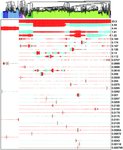
Figure 2: An illustration of some eigenvectors of ${\mathbf{\bolds{\Sigma}}}$ for the intestinal data. Only 25 of the 395 eigenvectors are shown: those that correspond to the first five largest eigenvalues, the last two smallest eigenvalues, and then a random sample in between. Each row represents an eigenvector, and the value of each element of the vector is plotted alongside the phylotype with which it corresponds. Blue represents a positive value, red a negative. The width indicates the absolute value of the element. Again, each row has been normalized so that the maximum width is the same in each row. Next to each row is printed the corresponding eigenvalue.

Several authors in phylogenetics have asserted that the eigenvectors of ${\mathbf{\bolds{\Sigma}}}$ have this multiscale structure [e.g., Cavalli-Sforza and Piazza (1975); Rohlf (2001); Martins and Housworth (2002)], but only limited statements of this kind can be rigorously made about a phylogenetic tree with more than four leaves/species [see Purdom (2006) for a longer discussion]. But empirical observations of the eigenvectors show that they often do have some characteristics of this multiscale property; for example, ${\mathbf{\bolds{\Sigma}}}$ has a block structure which guarantees that the eigenvectors of ${\mathbf{\bolds{\Sigma}}}$ will, at a minimum, be nonzero for only one side or the other of the initial split in the tree (Appendix E). Beyond this, if we ignore the comparatively small values in the eigenvector, eigenvectors corresponding to smaller eigenvalues do tend to divide the species into smaller and smaller closely-related groups based on the sign of the entries, though the groups do not exactly correspond to subtrees (see Figure 2).

6 gPCA applied to bacterial data and phylogenetic tree

In Eckburg et al. (2005) our original analysis of the bacterial data was a gPCA of $({\mathbf{\tilde{X}}},\bolds{\Sigma},{\mathbf{D}}_{\mathbf{w}_{{L}}})$, which is equivalent to DPCoA choosing ${\mathbf{\bolds\delta}}$ to be the distance among the phylotypes. We display in Figure 3 the ordination of the locations (samples) and species using the first two coordinates (using the implementation of DPCoA in the ade4 package in R [Chessel et al. (2005); R Development Core Team (2008)]). The first obvious fact is that the patients are separated, almost entirely, by just their value when projected onto the first axis. The first axis orders the patients B, C, A, which correlates with visual examination of the data in Figure 1. Below we will compare to other common choices of metrics and we will see that distinguishing the patients is not difficult since all of the techniques accomplish this, though not always in just one dimension. More interestingly, we also see in Figure 3 that the stool samples are distinguished from the internal biopsies of the colon, and the second axis seems to make this distinction. Again this makes sense from visually examining the data, since within each patient the stool samples do stand out from the biopsies.

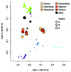
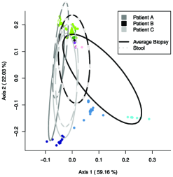
(a)	(b)

Figure 3: Scatter plot of the species and samples with the first two coordinates given by DPCoA. Species are shown as colored points in both plots. In plot (a), the samples are shown as the large blue shapes: different shapes indicate different patients and different shades of blue indicate location within the colon. In plot (b), samples are represented as ellipses that indicate the major directions of the abundances of the samples. For simplicity, a single ellipse for the combined abundance in the biopsies is shown because the internal biopsies are very similar.

The most striking aspect of the plot from the gPCA is the additional information provided from the inclusion of the phylotypes in the plot. Recall that when our data matrix ${\mathbf{X}}$ consists of profile vectors, our original axes ${\mathbf{e}_{{s}}}$ correspond to a location that is entirely concentrated in phylotype $s$. The coordinates of the phylotypes given by gPCA will be the coordinates of our axis ${\mathbf{e}_{{s}}}$ centered and rotated like the observed profiles (see Appendix A). Looking at the ordination plot, we see that the phylotypes’ coordinates provide an interpretation for the first two dimensions. The phylotypes are in clusters much like the groupings on the tree—not surprising if we recall that in the full space the distances between the species are exactly the distances on the tree. What is interesting is how the clusters on the tree fill the space once projected into these two coordinates that preserve the Rao Dissimilarity among the locations. The distribution of the phylotypes indicate the importance of these clusters in determining the dissimilarity between the patients. Those far from the origin have more impact in defining the coordinates of the locations. We see the tension between the various Bacteroides (blue) and the rest of the tree.

Furthermore, we can interpret the relationship between the locations and the phylotypes. We see that patient B is comparatively much more in the direction of the Prevotallae-like bacteria (light blue), while the other two patients are more in the direction of the B. Vulgatus-like phylotypes (dark blue). Similarly, the biopsies are comparatively more heavily represented in the Bacteroides (blue) portion of the tree, while the stool samples are comparatively less so. Figure 3(b) depicts the different samples as ellipses with the axes of the ellipses determined by the relative proportion of the different species for the location (see Appendix F). This illustration emphasizes that the samples can be thought of giving weights to each phylotype, and the ellipse demonstrates the relative influence of the different species. We see graphically the different influences of the two groups of Bacteriodes (blue) in separating the biopsies of patient B from all of the rest of the samples. Transforming the data in various ways before analysis does not dramatically change these relationships (e.g., log-transforming the data or adding pseudo-counts).

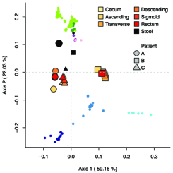
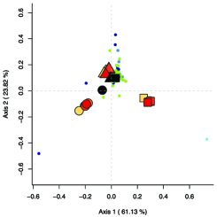
(a) gPCA with Tree / DPCoA	(b) NSCA (Gini–Simpson Distance)
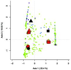
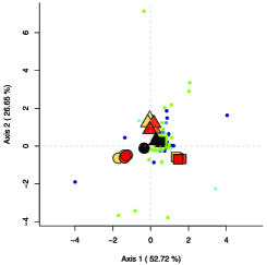
(c) CA	(d) gPCA with ${\mathbf{\bolds{\Sigma}}}^{-1}$

Figure 4: Coordinates of species and samples from alternative ordination techniques.

All of these visualizations have, by necessity, focused on only the first two dimensions of the coordinates given by gPCA. These dimensions do cover a large proportion of the Rao Dissimilarity, but still are only an approximation of the full space. We are mainly focused on demonstrating the characteristics of the ordination procedure in terms of the coordinate system that it creates, but for more rigorous testing of differences between the patients or between the biopsies and stool samples, permutation tests based on the $F$-statistic described above would generally want to compare with the entire coordinate system.

6.1 Comparison to other approaches

How do these results compare to the other ordination techniques mentioned above? In Figure 4 we show the results of the ordination from Non-symmetric Correspondence Analysis (NSCA), Correspondence Analysis (CA) and a Mahalanobis-like distance based on ${\mathbf{\bolds{\Sigma}}}^{-1}$ (see Section 5). We similarly center, rotate and project the axes ${\mathbf{e}_{{s}}}$ to get the species coordinates in the same manner as DPCoA.

As we mentioned, all of the techniques separate the three patients, but we see that the gPCA using the tree gives much more relevant results, both in terms of the role of the species and in relating to our intuitive interpretation of the data. The NSCA [plot (b)] is the same technique as our gPCA but with each species at equal distance from every other; it is also just a standard PCA with weights on the observations. In the first two coordinates of the NSCA, we see that instead of having a smooth contribution from clusters of phylotypes, two individual phylotypes, far removed from the rest, contribute to the division of the patients much more than the rest. The bulk of the species have little contribution to these coordinates. Thus, there is little from which to draw more general conclusions regarding the biological characteristics of the species which are influential. This is a consequence of treating each phylotype equally, rather than using the additional structure of the tree to shape the analysis. CA [Figure 4(c)], on the other hand, spreads out the importance of each phylotype. Here we can see the effect of the down-weighting metric in CA discussed earlier; differences found in the many low abundance phylotypes are allowed to influence the analysis. Rather than a couple of phylotypes dominating the analysis, as in NSCA, the phylotypes play more equal roles.

We might try to use any one of these techniques to reason out relationships among the variables. Each technique would give a different story in the role of the variables (phylotypes) dependent upon the assumptions inherent in the method. The relevant feature for our analysis is that we presuppose that a certain type of information is relevant—namely, how the structure of the tree relates to the data. This approach focuses the analysis on finding an interpretation among the variables that follows the tree structure.

We note that the abundance table from metagenomic studies discussed here has many features common to high-throughput experiments in biology—in particular, the number of biological samples is quite low compared to the number of measurements. We sought to integrate the phylogenetic information into the data analysis a priori. In this way, the analysis is constrained in a biologically relevant direction. In contrast, we could think of analyzing this abundance data much like a microarray experiment: test each phylotype individually for differences between the patients and use multiple testing criteria to identify individual phylotypes showing significant differences. A problem with this approach, which is also a common problem in microarrays analyses, would be that a list of significant phylotypes is difficult to interpret. In microarray studies, biological interpretation is often done a posteriori by then examining biological knowledge of the list of genes. We could similarly use the phylogenetic tree in this way. However, we just saw that an analysis independent of the tree highlighted only a couple of specific phylotypes from which it would be difficult to build a general connection to the tree.

6.2 Effect of the choice of metric

We can see the effect of using ${\mathbf{\bolds{\Sigma}}}$ in our gPCA by examining the linear combinations that gPCA using ${\mathbf{\bolds{\Sigma}}}$ chooses. For any ordination technique, let ${\mathbf{V}}$ be a matrix that rotates the original profiles ${\mathbf{X}}$ to give us the final ordination; in gPCA of centered data, this will be the matrix ${\mathbf{P}}_{\mathbf{w}_{S}}{\mathbf{Q}}_{S}{\mathbf{A}}$. We examine the different linear transformations, ${\mathbf{v}_{{i}}}$, from gPCA with ${\mathbf{\bolds{\Sigma}}}$ as compared to the transformation for a standard PCA on the data ${\widetilde{{\mathbf{X}}}}$ (equivalently, NSCA). And we also compare to the eigenvectors of ${\mathbf{\bolds{\Sigma}}}$: if the covariance between the species was exactly the ${\mathbf{\bolds{\Sigma}}}$ predicted by the evolution model, then these would be the principal components of such data. Thus, we can think of the eigenvectors of ${\mathbf{\bolds{\Sigma}}}$ as PCA on the tree.

Figure 5: Shown are the first five linear combinations of gPCA using ${\mathbf{\bolds{\Sigma}}}$ that act on the observations in ${\mathbf{X}}$ (the location profiles) to create the first five coordinates (${\mathbf{v}_{{i}}}$). The five dimensions are divided by thick, dotted line. Also shown adjacent to each gPCA vector are the linear combinations from a standard PCA of ${\widetilde{{\mathbf{X}}}}$ (labeled ‘X’) and the eigenvectors of ${\mathbf{\bolds{\Sigma}}}$ (labeled ‘${\mathbf{\bolds{\Sigma}}}$’).

In Figure 5 we order the elements of ${\mathbf{v}_{{i}}}$ from these three ordination techniques so that they line up with the phylogenetic tree. In this way we can see the relative importance of the phylotypes in transforming the data. When we look at the linear combinations for the first few coordinates, we see that the principal components from our gPCA with ${\mathbf{\bolds{\Sigma}}}$ intuitively seem to be a trade-off between these two options, and we could think of this as a shrinking of the data variability in the “direction” of the tree. This is a particularly appealing idea, since we are treating the phylotypes as variables and there are far too many variables for the number of samples we have.

Despite the intuitive results, the analysis depends on our choice of encoding the tree using ${\mathbf{\bolds{\Sigma}}}$ (or, equivalently, for DPCoA, our choice of ${\mathbf{\bolds\delta}}$). In particular, the block structure of ${\mathbf{\bolds{\Sigma}}}$ puts large emphasis on the first initial partition of the species at the root of the tree; these two groups of species are considered independent, conditional on the root ancestor. We can see this emphasis on this first divide from the Rao Dissimilarity based on ${\mathbf{\bolds\delta}}$, where these two lineages will be far away from each other and, thus, differences between will be accorded more weight in the analysis. However, as mentioned above, we see that the method depends only on ${\mathbf{\bolds\delta}}$, so the definition of the root of the tree, per se, is not the deciding factor, but rather the large amount of distance between these two subtrees.

Changes near the tips of the tree, both in the numerical data and the definition of the tree, will have little impact on the gPCA. For the bacterial data that we are interested in, the deeper tree structure is more trustworthy than the structure near the leaves of the tree because of the approximate definition of species. It is a reasonable compromise to put more weight on the deeper structure of the tree, and base our analysis on this dependence, in exchange for resolving the more fundamental problem in our definition of the species.

7 General graphs

It is clear that the same approach is applicable to other situations where there is complicated information that is related to the experimental data. By understanding our phylogenetic analysis as a specific example in a general approach to data analysis, we can compare with other techniques as well as take advantage of insights from other data situations.

A closely related example is when we have not a phylogenetic tree, but a more general graph structure that describes the relationship of our variables or observations. The analysis of experimental data in tandem with related biological networks by Rapaport et al. (2007) is equivalent to our metric approach. There, the authors used the Laplacian matrix associated with a graph to represent the biological graphs that related genes, where the the laplacian matrix ${\mathbf{L}}$ is given by ${\mathbf{D}}_{{\mathbf{d}}}-{\mathbf{A}}$, where ${\mathbf{A}}$ is the adjacency matrix of the graph and ${\mathbf{d}}$ is the vector of degrees of each node. The Laplacian matrix is a natural choice for graphs; the eigenvectors have similar multiscale properties as our metric for the phylogenetic tree. In Appendix D we briefly discuss the possibility of treating the phylogenetic tree as a general graph and using the Laplacian as a metric. We chose another approach here because such a choice does not well reflect the phylogenetic information in the tree.

A related application is found in spatial analysis, where spatial relationships between observations are based on neighborhood relationships, or, more generally, distances between points. While many analyses first remove the spatial dependencies so as to have independent observations, it is often also of interest to evaluate the relationship between the spatial patterns and the observed data. When spatial connectivity between observations is simplified to a zero–one connectivity measure (usually based on a cutoff on the distance between the observations), the spatial relationship is given by an adjacency matrix. Geary’s $c$ and Moran’s $I$, two common measures of the spatial autocorrelation of ${\mathbf{y}}\in\mathbb{R}^{n}$ (a variable observed on the $n$ observations), can be written in terms of the adjacency matrix [Thioulouse, Chessel and Champely (1995)],

$$c = \frac{(n-1)\sum_{j=1}^{n}\sum_{j=1}^{n}{\mathbf{A}_{(ij)}}({\mathbf{y}_{{}{(i)}}}-{\mathbf{y}_{{}{(j)}}})^{2}}{2N_{e}\sum_{i}({\mathbf{y}_{{}{(i)}}}-\bar{y})^{2}}=\frac{n-1}{N_{e}}\frac{{\mathbf{\tilde{y}}}^{T}({\mathbf{D}}_{{\mathbf{d}}}-{\mathbf{A}}){\mathbf{\tilde{y}}}}{{\mathbf{\tilde{y}}}^{T}{\mathbf{\tilde{y}}}},$$

$$I = \frac{(n)\sum_{j=1}^{n}\sum_{j=1}^{n}{\mathbf{A}_{(ij)}}({\mathbf{y}_{{}{(i)}}}-\bar{y})({\mathbf{y}_{{}{(j)}}}-\bar{y})}{2N_{e}\sum_{i}({\mathbf{y}_{{}{(i)}}}-\bar{y})^{2}}=\frac{n}{N_{e}}\frac{{\mathbf{\tilde{y}}}^{T}{\mathbf{A}}{\mathbf{\tilde{y}}}}{{\mathbf{\tilde{y}}}^{T}{\mathbf{\tilde{y}}}},$$

where ${\mathbf{\tilde{y}}}={\mathbf{y}}-\bar{y}{\mathbf{1}_{{n}}}$ is ${\mathbf{y}}$ centered by the standard (unweighted) mean of the elements of ${\mathbf{y}}$ and $N_{e}=\sum_{ij}{\mathbf{A}_{ij}}$ is twice the number of edges in the graph. In particular, we see that Geary’s $c$ can be written in terms of an inner-product using the Laplacian.

Thioulouse, Chessel and Champely (1995) note that the variance of ${\mathbf{y}}$ with observations weighted by their node-degree, given by $\operatorname{var}_{{\mathbf{D}}_{{\mathbf{d}}}}({\mathbf{y}})={\mathbf{\tilde{y}}}^{T}{\mathbf{D}}_{{\mathbf{d}}}{\mathbf{\tilde{y}}}/N_{e}$, can be decomposed into related components,

$$\operatorname{var}_{{\mathbf{D}}_{{\mathbf{d}}}}({\mathbf{y}})={\mathbf{\tilde{y}}}^{T}\frac{{\mathbf{D}}_{{\mathbf{d}}}-{\mathbf{A}}}{N_{e}}{\mathbf{\tilde{y}}}+{\mathbf{\tilde{y}}}^{T}\frac{{\mathbf{A}}}{N_{e}}{\mathbf{\tilde{y}}}.$$

Thus, Geary’s $c$ and Moran’s $I$ are similar to $F$ measures described above, that is, the ratio of component variability to total variability (note, however, that Moran’s $I$ can be negative). Several authors have proposed spatial multivariate analyses which rely on ${\mathbf{L}}$ as a metric for the rows, or a row standardized version ${\mathbf{L}}^{*}={\mathbf{D}}_{{\mathbf{d}}}^{-1}({\mathbf{D}}_{{\mathbf{d}}}-{\mathbf{A}})$ [Aluja-Ganet and Nonell-Torrent (1991); Thioulouse, Chessel and Champely (1995); di Bella and Jona-Lasinio (1996); Dray, Saïd and Debias (2008)]. [Note that the matrix ${\mathbf{L}}^{*}$ as well as the similar matrix ${\mathbf{\widetilde{L}}}={\mathbf{D}}_{{\mathbf{d}}}^{-1/2}({\mathbf{D}}_{{\mathbf{d}}}-{\mathbf{A}}){\mathbf{D}}_{{\mathbf{d}}}^{-1/2}$ are also considered in graph theory; see Biyikoğlu, Leydold and Stadler (2007).]

8 Conclusion

There is a clear necessity for including phylogenetic information in an analysis of metagenomic data. gPCA gives a simple and compelling way to accomplish this. We also see from our recasting of DPCoA as a gPCA that the framework of gPCA allows for easy comparisons between seemingly disparate analyses as well as further exploration as to the effect of our choice of metrics.

The use of nonstandard metrics is quite natural in statistics and can be implemented in a variety of ways, PCA being merely the simplest. Common examples, such as Mahalanobis distance, are usually data-driven, but we see that metrics based on outside knowledge can be used to include complicated and heterogeneous information into the analysis of our numerical data. This kind of information can help to give more context to the data, particularly when the number of variables is large as compared to the samples. Moreover, since the metrics here correspond to covariance matrices, probabilistic models give a simple approach for encoding information appropriately. Often, as in the case of phylogenetic trees, the eigenvectors of such covariance matrices have nice localization properties that highlight the relevant spatial or regional patterns of the prior information.

Appendix A DPCoA and gPCA

We state here the equivalence between DPCoA and gPCA described in Section 3.3. First we describe more explicitly DPCoA, as described in Pavoine, Dufour and Chessel (2004).

DPCoA. Assume that the squared pairwise distances/dissimilarities between the species are given by a $S\times S$ matrix ${\mathbf{\bolds\delta}}$. We also assume that the distances are Euclidean (i.e., coordinates can be found for the points so that the standard Euclidean distance between points is given by the square-root of the entries of ${\mathbf{\bolds\delta}}$).

Following the notation provided in Section 4, let ${\mathbf{P}}_{{\mathbf{w}_{{m}}}}=({\mathbf{I}}_{m}-{\mathbf{1}_{{m}}}\mathbf{w}_{m}^{T})$ be the projection matrix that centers $m$ observations based on a weighted mean with ${\mathbf{w}_{{m}}}$ as weights:

1. [3.]

2. Find Euclidean coordinates of the species using a weighted version of Multidiminsional Scaling, with weights for the species given by $\mathbf{w}_{S}$, typically [and as proposed by Pavoine, Dufour and Chessel (2004)] the relative abundance of the species in all the samples. Specifically, let ${\mathbf{U}}$ be the eigenvectors of

   $$\mathbf{D}_{\mathbf{w}_{S}}^{1/2}{\mathbf{P}}_{\mathbf{w}_{S}}(-{\mathbf{\bolds\delta}}/2){\mathbf{P}}_{\mathbf{w}_{S}}^{T}\mathbf{D}_{\mathbf{w}_{S}}^{1/2}.$$

   Then the new coordinates of the species are given by the rows of ${\mathbf{Z}}\in\mathbb{R}^{S\times s^{*}}$ ($s^{*}\leq S-1$ is the dimension of the space required to contain the species). Then we have ${\mathbf{Z}}=\mathbf{D}_{\mathbf{w}_{S}}^{-1/2}{\mathbf{U}}\bolds{\Lambda}^{1/2}$. Note that we could also start with a similarity matrix between species, ${\mathbf{S}}_{{\mathbf{v}}}={\mathbf{1}}{\mathbf{v}}^{T}+{\mathbf{v}}{\mathbf{1}}^{T}-\frac{1}{2}{\mathbf{\bolds\delta}}$ for any ${\mathbf{v}}$ that implies ${\mathbf{S}}_{{\mathbf{v}}}$ is positive definite. Because

   $${\mathbf{P}}_{{\mathbf{w}}}{\mathbf{S}}_{{\mathbf{v}}}{\mathbf{P}}_{{\mathbf{w}}}^{T}={\mathbf{P}}_{{\mathbf{w}}}(-{\mathbf{\bolds\delta}}/2){\mathbf{P}}_{{\mathbf{w}}}^{T}$$

   for any weights ${\mathbf{w}}$ and vector ${\mathbf{v}}$ the MDS will be equivalent. This is, of course, the standard equivalence between starting with a similarity matrix or dissimiliarity matrix in MDS.

3. Set the coordinates of the locations to be at the barycenter of the species coordinates. In other words, each location $\ell$ is given coordinates that are the weighted average of the coordinates of all the species and the weights are given by the relative abundance of the species in that site (which is contained in the vector ${\mathbf{x}_{{\ell}}}$). Let the rows of the ${L}\times s^{*}$ matrix ${\mathbf{Y}}$ contain the coordinates of the sites, so

   $${\mathbf{Y}}={\mathbf{X}}{\mathbf{Z}}.$$

   The squared pairwise Euclidean distance between the locations using these coordinates will be equal to their Rao Dissimilarity using the dissimilarity matrix ${\mathbf{\bolds\delta}}$.

4. Find a lower-dimensional representation of the locations using a generalized principal components analysis on the triplet $({\mathbf{Y}},{\mathbf{I}}_{S},\mathbf{D}_{\mathbf{w}_{{L}}})$, where $\mathbf{D}_{\mathbf{w}_{{L}}}$ is a diagonal matrix consisting of weights for the locations, $\mathbf{w}_{{L}}$ (again, typically the relative abundance of the locations in all the samples). Let $r=\operatorname{rank}({\mathbf{Y}})$. Then gPCA of $({\mathbf{Y}},{\mathbf{I}}_{S},\mathbf{D}_{\mathbf{w}_{{L}}})$ gives the eigenvalue equations,

   $${\mathbf{Y}}^{T}\mathbf{D}_{\mathbf{w}_{{L}}}{\mathbf{Y}}{\mathbf{F}}={\mathbf{F}}\bolds{\Phi},\qquad{\mathbf{Y}}{\mathbf{Y}}^{T}\mathbf{D}_{\mathbf{w}_{{L}}}{\mathbf{G}}={\mathbf{G}}\bolds{\Phi},$$

   (1)

   $$\eqntext{\mbox{where }{\mathbf{F}}^{T}{\mathbf{F}}={\mathbf{I}}_{r},\ {\mathbf{G}}^{T}\mathbf{D}_{\mathbf{w}_{{L}}}{\mathbf{G}}={\mathbf{I}}_{r}}$$ (2)

   and ${\mathbf{Y}}={\mathbf{G}}\bolds{\Phi}^{1/2}{\mathbf{F}}^{T}$ is the generalized SVD decomposition of ${\mathbf{Y}}$. The final coordinates of the locations are given by

   $${\mathbf{L}}={\mathbf{Y}}{\mathbf{F}}.$$

   We also transform the coordinates of the species to get species coordinates (see Section 4.2),

   $${\mathbf{K}}={\mathbf{Z}}{\mathbf{F}}.$$

The coordinates for the locations given by ${\mathbf{L}}$ in DPCoA using ${\mathbf{\bolds\delta}}$ are equivalent to the coordinates ${\mathbf{\widehat{X}}}={\widetilde{{\mathbf{X}}}}{\mathbf{S}}_{{\mathbf{v}}}{\mathbf{A}}$ of the locations given by gPCA with the triplet $({\widetilde{{\mathbf{X}}}},{\mathbf{S}}_{{\mathbf{v}}},\mathbf{D}_{\mathbf{w}_{{L}}})$, where ${\widetilde{{\mathbf{X}}}}={\mathbf{X}}{\mathbf{P}}_{\mathbf{w}_{S}}$ is the column centered matrix of data. Furthermore, the coordinates of the species given by DPCoA in the matrix ${\mathbf{K}}$ are equivalent to the coordinates obtained by centering and then rotating the original axes ${\mathbf{e}_{{s}}}$ by the transformation implied from the gPCA of $({\widetilde{{\mathbf{X}}}},{\mathbf{S}}_{{\mathbf{v}}},\mathbf{D}_{\mathbf{w}_{{L}}})$ so that ${\mathbf{K}}={\mathbf{P}}_{\mathbf{w}_{S}}{\mathbf{S}}_{{\mathbf{v}}}{\mathbf{A}}$.

The fundamental eigenequations for a gPCA of the triplet $({\mathbf{\widetilde{{\mathbf{X}}}}},\allowbreak{\mathbf{S}}_{{\mathbf{v}}},\mathbf{D}_{\mathbf{w}_{{L}}})$ are

$${\mathbf{\widetilde{{\mathbf{X}}}}}^{T}\mathbf{D}_{\mathbf{w}_{{L}}}{\mathbf{\widetilde{{\mathbf{X}}}}}{\mathbf{S}}_{{\mathbf{v}}}{\mathbf{A}}={\mathbf{A}}\bolds{\Psi},\qquad{\mathbf{\widetilde{{\mathbf{X}}}}}{\mathbf{S}}_{{\mathbf{v}}}{\mathbf{\widetilde{{\mathbf{X}}}}}^{T}\mathbf{D}_{\mathbf{w}_{{L}}}{\mathbf{{\mathbf{B}}}}={\mathbf{{\mathbf{B}}}}\bolds{\Psi},$$

(3)

$$\eqntext{\mbox{where }{\mathbf{A}}^{T}{\mathbf{S}}_{{\mathbf{v}}}{\mathbf{A}}={\mathbf{I}}_{r},\ {\mathbf{{\mathbf{B}}}}^{T}\mathbf{D}_{\mathbf{w}_{{L}}}{\mathbf{{\mathbf{B}}}}={\mathbf{I}}_{r},}$$ (4)

so that ${\mathbf{X}}{\mathbf{P}}_{\mathbf{w}_{S}}={\mathbf{{\mathbf{B}}}}\bolds{\Psi}^{1/2}{\mathbf{A}}^{T}$ is the corresponding gSVD.

Since ${\mathbf{\widetilde{{\mathbf{X}}}}}={\mathbf{X}}{\mathbf{P}}_{\mathbf{w}_{S}}$, we see that ${\mathbf{{\mathbf{B}}}}$ and ${\mathbf{G}}$ from DPCoA are both eigenvectors for the same matrix, ${\mathbf{X}}{\mathbf{P}}_{\mathbf{w}_{S}}{\mathbf{S}}_{{\mathbf{v}}}{\mathbf{P}}_{\mathbf{w}_{S}}^{T}{\mathbf{X}}^{T}\mathbf{D}_{\mathbf{w}_{{L}}}$, implying that ${\mathbf{{\mathbf{B}}}}$ and ${\mathbf{G}}$ are the $\mathbf{D}_{\mathbf{w}_{{L}}}$-orthonormal eigenvectors of the same matrix. This implies that the eigenvalues are the same ($\bolds{\Phi}=\bolds{\Psi}$) and that ${\mathbf{{\mathbf{B}}}}$ and ${\mathbf{G}}$ are the same up to a sign change (assuming unique eigenvalues).

The resulting coordinates for the locations under DPCoA are given by ${\mathbf{L}}={\mathbf{Y}}{\mathbf{F}}={\mathbf{G}}\bolds{\Phi}^{1/2}.$ With gPCA of $({\mathbf{\widetilde{{\mathbf{X}}}}},{\mathbf{S}}_{{\mathbf{v}}},\mathbf{D}_{\mathbf{w}_{{L}}})$, the location coordinates are ${\mathbf{\widehat{X}}}={\mathbf{X}}{\mathbf{P}}_{\mathbf{w}_{S}}{\mathbf{S}}_{{\mathbf{v}}}{\mathbf{A}}={\mathbf{{\mathbf{B}}}}\bolds{\Psi}^{1/2}$ and, therefore, we have that ${\mathbf{L}}={\mathbf{\widehat{X}}}$—the coordinates of the locations are the same in the two methods.

The coordinates for the species are given by DPCoA as the rotation of the coordinates given in ${\mathbf{Z}}$ by ${\mathbf{F}}$: ${\mathbf{K}}={\mathbf{Z}}{\mathbf{F}}$. By the gSVD decomposition of ${\mathbf{Y}}$, we can write ${\mathbf{F}}^{T}=\bolds{\Phi}^{-1/2}{\mathbf{G}}^{T}\mathbf{D}_{\mathbf{w}_{{L}}}{\mathbf{Y}}$ and, similarly, ${\mathbf{{\mathbf{B}}}}\bolds{\Psi}^{-1/2}={\mathbf{X}}{\mathbf{P}}_{\mathbf{w}_{S}}{\mathbf{S}}_{{\mathbf{v}}}{\mathbf{A}}\bolds{\Psi}^{-1}$. Remembering that ${\mathbf{Z}}{\mathbf{Z}}^{T}={\mathbf{P}}_{\mathbf{w}_{S}}{\mathbf{\bolds\delta}}{\mathbf{P}}_{\mathbf{w}_{S}}^{T}$, the final coordinates of the species from DPCoA are given by

$${\mathbf{K}} = {\mathbf{Z}}{\mathbf{Y}}^{T}\mathbf{D}_{\mathbf{w}_{{L}}}{\mathbf{G}}\bolds{\Phi}^{-1/2}={\mathbf{Z}}{\mathbf{Z}}^{T}{\mathbf{X}}^{T}\mathbf{D}_{\mathbf{w}_{{L}}}{\mathbf{G}}\bolds{\Phi}^{-1/2}$$

$$= {\mathbf{P}}_{\mathbf{w}_{S}}{\mathbf{\bolds\delta}}{\mathbf{P}}_{\mathbf{w}_{S}}^{T}{\mathbf{X}}^{T}\mathbf{D}_{\mathbf{w}_{{L}}}{\mathbf{G}}\bolds{\Phi}^{-1/2}$$

$$= {\mathbf{P}}_{\mathbf{w}_{S}}{\mathbf{S}}_{{\mathbf{v}}}\underbrace{{\mathbf{P}}_{\mathbf{w}_{S}}^{T}{\mathbf{X}}^{T}\mathbf{D}_{\mathbf{w}_{{L}}}{\mathbf{X}}{\mathbf{P}}_{\mathbf{w}_{S}}{\mathbf{S}}_{{\mathbf{v}}}{\mathbf{A}}}_{={\mathbf{A}}\bolds{\Psi}\mathrm{\ from\ {{(\ref{eq:tcoveigeneq})}}}}\bolds{\Psi}^{-1}={\mathbf{P}}_{\mathbf{w}_{S}}{\mathbf{S}}_{{\mathbf{v}}}{\mathbf{A}}$$

up to the sign change difference between ${\mathbf{G}}$ and ${\mathbf{{\mathbf{B}}}}$.

Appendix B Kernel analysis and gPCA

Multivariate kernel methods seek a set of functions $f_{1},\ldots,f_{k}$ from our general data space ${\mathcal{X}}$ into $\mathbb{R}$, such that the possible set of functions $f$ form a Reproducing Kernel Hilbert Space with respect to a kernel function ${\mathcal{K}}$ on ${\mathcal{X}}$ [see Schölkopf and Smola (2002) for details]. The solutions for a multivariate Kernel CCA (or extensions) can be recovered from the eigenequations, assuming ${\mathbf{K}}_{i}$ are invertible

$${\mathbf{K}}_{\xi_{2}}^{-1}{\mathbf{K}}_{2}{\mathbf{K}}_{1}{\mathbf{U}}_{1}={\mathbf{K}}_{\xi_{1}}{\mathbf{U}}_{1}\bolds{\Lambda}$$

with the constraint that

$${\mathbf{U}}_{i}^{T}{\mathbf{K}}_{\xi_{i}}{\mathbf{U}}_{i}=\bolds{\Gamma}_{i}$$

and ${\mathbf{U}}_{2}$ is given by

$${\mathbf{U}}_{2}={\mathbf{K}}_{\xi_{2}}^{-1}{\mathbf{K}}_{1}{\mathbf{U}}_{1}(\bolds{\Lambda}\bolds{\Gamma}_{1}\bolds{\Gamma}_{2}^{-1})^{-1/2},$$

where ${\mathbf{K}}_{\xi_{i}}=(1-\xi_{i}){\mathbf{K}}_{i}/n+\xi_{i}{\mathbf{I}},$ and $\bolds{\Gamma}_{i}$ are diagonals of normalization constants chosen by the user. Then the new coordinates of an object $x$ from data set $i$ are given by $(f_{1}(x),\ldots,f_{k}(x))^{T}={\mathbf{k}}^{T}{\mathbf{U}}_{i}$, where ${\mathbf{k}_{{}{(j)}}}={\mathcal{K}}_{i}(x,x_{j})$.

Let ${\mathbf{K}}_{1}={\mathbf{Q}}_{{n}},$ ${\mathbf{K}}_{2}={\mathbf{X}}{\mathbf{Q}}_{{p}}{\mathbf{X}}^{T},$ and $\xi_{1}=\xi_{2}=1$, then we have the eigenequation

$${\mathbf{X}}{\mathbf{Q}}_{{p}}{\mathbf{X}}^{T}{\mathbf{Q}}_{{n}}{\mathbf{U}}_{1}={\mathbf{U}}_{1}\bolds{\Lambda}.$$ (5)

We see that these are equivalent to the gPCA equations, with ${\mathbf{U_{1}}}={\mathbf{B}}$. Then the coordinates associated with the data matrix ${\mathbf{X}}$ from the kernel method are

$${\mathbf{K}}_{2}{\mathbf{U}}_{2}={\mathbf{K}}_{2}{\mathbf{K}}_{1}{\mathbf{U}}_{1}(\bolds{\Lambda}\bolds{\Gamma}_{1}\bolds{\Gamma}_{2}^{-1})^{-1/2}={\mathbf{X}}{\mathbf{Q}}_{{p}}{\mathbf{X}}^{T}{\mathbf{Q}}_{{n}}{\mathbf{U}}_{1}\bolds{\Lambda}^{-1/2}(\bolds{\Gamma}_{1}\bolds{\Gamma}_{2}^{-1})^{-1/2},$$

while those from the gPCA are

$${\mathbf{X}}{\mathbf{Q}}_{{p}}{\mathbf{A}}={\mathbf{X}}{\mathbf{Q}}_{{p}}{\mathbf{X}}^{T}{\mathbf{Q}}_{{n}}{\mathbf{B}}\bolds{\Lambda}^{-1/2}.$$

Choosing the scaling of the eigenvectors so that $(\bolds{\Gamma}_{1}\bolds{\Gamma}_{2}^{-1})={\mathbf{I}}$ makes the solutions equivalent.

Appendix C Inertia and dissimilaries

We generalize the results of Pélissier et al. (2003) to show the derivation of the dissimilarity and diversity results above.

In gPCA, the term inertia is used for the inter-point similarities, and the total inertia between points is defined as $I({\mathbf{X}},{\mathbf{Q}}_{{p}},{\mathbf{Q}}_{{n}})=\operatorname{tr}({\mathbf{Q}}_{{n}}{\mathbf{X}}{\mathbf{Q}}_{{p}}{\mathbf{X}}^{T})=\sum\lambda_{i}.$ Then if ${\mathbf{\widehat{X}}}_{(r)}$ are the new coordinates of ${\mathbf{X}}$ restricted to the first $r$ dimensions and ${\mathbf{\widehat{X}}}_{(-r)}$ the remaining ${p}-r$ dimensions, we can decompose the total inertia into the inertia of the first $r$ dimensions and that of the remaining ${p}-r$,

$$I({\mathbf{X}},{\mathbf{Q}}_{{p}},{\mathbf{Q}}_{{n}}) = I\bigl{(}{\mathbf{\widehat{X}}}_{(r)},{\mathbf{I}}_{p},{\mathbf{Q}}_{{n}}\bigr{)}+I\bigl{(}{\mathbf{\widehat{X}}}_{(-r)},{\mathbf{I}}_{p},{\mathbf{Q}}_{{n}}\bigr{)}$$

$$= \sum_{i=1}^{r}\lambda_{i}+\sum_{i=r+1}^{p}\lambda_{i},$$

and the first $r$ dimensions give maximal possible inertia for $r$ dimensions.

Let ${\mathbf{Y}}\in\mathbb{R}^{N\times S}$ be the incidence matrix for the species variable, where ${\mathbf{Y}}_{(is)}$ is an indicator of the $i$th observation being species $s$. Let ${\mathbf{Z}}\in\mathbb{R}^{N\times{L}}$ be a similar such incidence matrix for the location variable. Then the inertia of the eigenanalysis of the triplet $({\mathbf{\widetilde{Y}}},{\mathbf{Q}},{\mathbf{D}}_{N})$, where ${\mathbf{\widetilde{Y}}}$ is the (nonweighted) centered ${\mathbf{Y}}$ and ${\mathbf{D}}_{N}$ is a diagonal matrix of $N$ elements, will be equal to $H_{{\mathbf{Q}}}({\mathbf{\bar{x}}})$. Regressing ${\mathbf{Y}}$ onto ${\mathbf{Z}}$ gives predictions ${\mathbf{\widetilde{Y}}}_{Z}$ and residuals ${\mathbf{\widetilde{Y}}}_{|Z}={\mathbf{\widetilde{Y}}}-{\mathbf{\widetilde{Y}}}_{Z}$. Then the total inertia ($I_{\mathrm{T}}$) can be broken into the inertia due to differences between locations ($I_{\mathrm{B}}$) plus the remaining inertia within locations ($I_{\mathrm{W}}$),

$$\operatorname{Inertia}({\mathbf{\widetilde{Y}}},{\mathbf{Q}},{\mathbf{D}}_{N})=\operatorname{Inertia}({\mathbf{\widetilde{Y}}}_{Z},{\mathbf{Q}},{\mathbf{D}}_{N})+\operatorname{Inertia}({\mathbf{\widetilde{Y}}}_{|Z},{\mathbf{Q}},{\mathbf{D}}_{N}).$$

Note that ${\mathbf{\widetilde{Y}}}_{Z}={\mathbf{Z}}{\widetilde{{\mathbf{X}}}}$, so that the inertia explained by ${\mathbf{Z}}$ is equal to the inertia of the eigenanalysis of ${\widetilde{{\mathbf{X}}}}$,

$$I_{\mathrm{B}}=\operatorname{Inertia}({\mathbf{\widetilde{Y}}}_{Z},{\mathbf{Q}},{\mathbf{D}}_{N})=\operatorname{Inertia}({\widetilde{{\mathbf{X}}}},{\mathbf{Q}},\mathbf{D}_{\mathbf{w}_{{L}}}).$$

This implies that the ordination procedures described above best preserve the between location dissimilarities defined by the metric ${\mathbf{Q}}$.

Appendix D The Laplacian and a Laplacian for trees

The Laplacian matrix that is associated with the graph is given by ${\mathbf{L}}={\mathbf{D}}-{\mathbf{A}}$, where ${\mathbf{A}}$ is the adjacency matrix of the graph and ${\mathbf{D}}$ is the diagonal matrix consisting of the degree of each vertex. The spectral decomposition of ${\mathbf{L}}$ is closely related to certain properties of the graph; in particular, there are many results linking the eigenvalues of ${\mathbf{L}}$ with fundamental characteristics of the graph [see Diestel (2005)]. There are fewer explicit characterizations of the eigenvectors that hold for all graphs. In a general way, the eigenvectors corresponding to small eigenvalues of ${\mathbf{L}}$ represent large divisions in the graph (indeed, for $\lambda_{0}=0$, we have the eigenvector ${\mathbf{1}}$ which is an average of all the nodes); they tend to be zero for large portions of the graph and the nonzero components are the same sign distinct regions of the graph. Those eigenvectors corresponding to large eigenvalues tend be dominated by linear combinations of “close” nodes or smaller groups of nodes and represent the “noisy,” small differences within neighboring vertices. Thus, the eigenvectors of the Laplacian have “multiscale” characteristics, particularly those eigenvectors corresponding to the largest and smallest of the eigenvalues. For data ${\mathbf{x}}$ associated with a graph, with each element of ${\mathbf{x}}$ corresponding to a node in the graph, the metrics for a graph based on the Laplacian will usually put greater weight on the eigenvectors corresponding to small eigenvalues, for example, $1/\lambda_{i}$ or $\exp(-1/\lambda_{i})$. This choice corresponds to the behavior of the eigenvectors.

The Laplacian gives the covariance between nodes from a useful model for describing relationships among the nodes—a model of diffusion of information through the graph. The covariance from this model is given by $\exp(-2\alpha{\mathbf{L}})$, known as the heat kernel of the graph [see Kondor and Lafferty (2002) for review]. Of course, this is equivalent to weighting the eigenvectors of the Laplacian with weight function $\exp(-\alpha\lambda_{i})$.

A phylogenetic tree is, of course, a graph, and the Laplacian of a tree and the distances between nodes on a tree are quite simply related [Bapat, Kirkland and Neumann (2005)]. Let ${\mathbf{\bolds\delta}}_{T}$ be the distance matrix of the patristic distances between all the nodes of the tree (internal nodes as well as the leaves), and let ${\mathbf{L}}$ be the Laplacian of the tree with weights $1/d(r,s)$ on each edge. Then we have that

$${\mathbf{L}}={\mathbf{v}}{\mathbf{v}}^{T}/\sum d(r,s)-2{\mathbf{\bolds\delta}}_{T}^{-1},$$

where for a phylogenetic tree ${\mathbf{v}}$ is $-1$ or $1$ depending on whether the node is a leaf of the tree or not.

However, since our data is observed on only certain nodes of the graph—the leaves of the tree—we need a metric that gives a relationship only between the leaves. If we use the Laplacian as our phylogenetic metric, we would have to constrain ourselves to the portion of the metric that corresponds to the relationships between just the leaves, ${\mathbf{L}}_{S}$. If we took as our metric the inverse of the Laplacian—which corresponds to an appropriate ordering of the eigenvectors by weighting each by $1/\lambda_{i}$—we have that ${\mathbf{L}}^{-1}_{S}$ is given by

$${\mathbf{L}}^{-1}_{S}=c{\mathbf{\bolds\gamma}}{\mathbf{\bolds\gamma}}^{T}-1/2{\mathbf{\bolds\delta}}_{S},\qquad\mbox{where }c=(8{\mathbf{1}}^{T}{\mathbf{\bolds\delta}}_{S\times I}{\mathbf{1}})^{-1},\ {\mathbf{\bolds\gamma}}={\mathbf{\bolds\delta}}_{T}{\mathbf{v}},$$

and ${\mathbf{\bolds\delta}}_{S}\in\mathbb{R}^{S\times S}$ is the distance matrix restricted to the distances between leaves of the tree and ${\mathbf{\bolds\delta}}_{SI}\in\mathbb{R}^{S\times S-1}$ is the distance matrix restricted to the distances between the leaves of the tree and $S-1$ internal nodes of the tree. This is an expression somewhat similar to our similarity matrix for DPCoA, but note that a gPCA based on ${\mathbf{L}}^{-1}_{S}$ is not equivalent to DPCoA because ${\mathbf{P}}{\mathbf{\bolds\gamma}}{\mathbf{\bolds\gamma}}{\mathbf{P}}^{T}$ does not vanish.

However, restricting the metric to those portions dealing only with the leaves makes the metric difficult to interpret. The Laplacian restricted to the leaves will no longer have the same eigenvectors as the Laplacian and thus loses its connection to the behavior shown by the eigenvectors of the Laplacian. Furthermore, from the point of view of covariance modeling, the phylogenetic tree represents an evolutionary story that is more directly modeled by ${\mathbf{\bolds{\Sigma}}}$.

Appendix E Eigenvectors of ${\mathbf{\bolds{\Sigma}}}$ for a phylogenetic tree

Note the block structure in ${\mathbf{\bolds{\Sigma}}}$: if the root ancestor, ${\mathcal{R}}$, has immediate descendants ${\mathcal{P}}_{1}$ and ${\mathcal{P}}_{2}$, then the covariance between any of the existing descendants of ${\mathcal{P}}_{1}$ and those of ${\mathcal{P}}_{2}$ will be $0$. Thus, we can order the rows and columns of ${\mathbf{\bolds{\Sigma}}}$ so that

$${\mathbf{\bolds{\Sigma}}}=\pmatrix{{\mathbf{\bolds{\Sigma}}}_{1}&{\mathbf{\bm{\varnothing}}}\cr{\mathbf{\bm{\varnothing}}}&{\mathbf{\bolds{\Sigma}}}_{2}},$$ (6)

where ${\mathbf{\bolds{\Sigma}}}_{1}$ is a $S_{1}\times S_{1}$ matrix, $S_{1}$ is the number of extant species descended from ${\mathcal{P}}_{1}$, and similarly with ${\mathbf{\bolds{\Sigma}}}_{2}$. This means that the eigenvectors of ${\mathbf{\bolds{\Sigma}}}$ must be of the form

$$\pmatrix{{\mathbf{v}_{{1i}}}\cr{\mathbf{\bm{\varnothing}}}}\quad\mbox{or}\quad\pmatrix{{\mathbf{\bm{\varnothing}}}\cr{\mathbf{v}_{{2j}}}},$$ (7)

where $\{{\mathbf{v}_{{1i}}}\}_{i=1}^{S_{1}}$ are the eigenvectors of ${\mathbf{\bolds{\Sigma}}}_{1}$ and $\{{\mathbf{v}_{{2j}}}\}_{j=1}^{S_{2}}$ are the eigenvectors of ${\mathbf{\bolds{\Sigma}}}_{2}$. Therefore, every eigenvector of ${\mathbf{\bolds{\Sigma}}}$, at a minimum, must be only nonzero for one of the lineages.

Indeed, if we think back to the definition of ${\mathbf{\bolds{\Sigma}}}$, the elements of the blocks ${\mathbf{\bolds{\Sigma}}}_{1},{\mathbf{\bolds{\Sigma}}}_{2}$ are themselves rank-1 perturbations of block diagonal matrices:

$${\mathbf{\bolds{\Sigma}}}_{1}=\pmatrix{{\mathbf{\bolds{\Sigma}}}_{11}&{\mathbf{\bm{\varnothing}}}\cr{\mathbf{\bm{\varnothing}}}&{\mathbf{\bolds{\Sigma}}}_{12}}+c_{1}{\mathbf{1}}{\mathbf{1}}^{T},\qquad{\mathbf{\bolds{\Sigma}}}_{2}=\pmatrix{{\mathbf{\bolds{\Sigma}}}_{21}&{\mathbf{\bm{\varnothing}}}\cr{\mathbf{\bm{\varnothing}}}&{\mathbf{\bolds{\Sigma}}}_{22}}+c_{2}{\mathbf{1}}{\mathbf{1}}^{T},$$ (8)

where $c_{1}={d_{\mathcal{T}}({\mathcal{R}},{\mathcal{P}}_{1})}$ and $c_{2}={d_{\mathcal{T}}({\mathcal{R}},{\mathcal{P}}_{2})}$ (here we have assumed that ${\mathbf{t}}\propto{\mathbf{1}}$ for simplicity). This same logic continues so that each sub-block can be written as a block matrix plus a rank-one perturbation. ${\mathbf{\bolds{\Sigma}}}$ thus consists of such nested rank-1 perturbations of block matrices.

The claims in the literature for a relationship of the eigenvectors of ${\mathbf{\bolds{\Sigma}}}$ to the partitions of the tree all stem from the comments of Cavalli-Sforza and Piazza (1975). They make assertions which they prove only in the case of a tree with four leaves ($S=4$) and under the assumption of a constant rate of evolution (${\mathbf{t}}\propto{\mathbf{1}}$). One assertion is true: for any terminal bifurcation node (a node whose two descendants are existing species or leaves of the tree), there is an eigenvector of ${\mathbf{\bolds{\Sigma}}}$ that has elements that are positive for one of the species, negative for the other and zero for all other species. In addition, we see that because of the block structure, every eigenvector of ${\mathbf{\bolds{\Sigma}}}$, at a minimum, must consist of zero elements for one branch of the tree.

Beyond this, Cavalli-Sforza and Piazza (1975) describe “usual” behavior of the eigenvectors, but their ideas do not scale as the size of the tree increases. The nested block structure of ${\mathbf{\bolds{\Sigma}}}$ still has the effect of creating eigenvectors with some structure to them, though not as easily classified as suggested in Cavalli-Sforza and Piazza (1975). Generally the structure of the eigenvectors will not be directly related to a partition in the tree. In practice, the eigenvectors often have some relation to the bifurcations of the tree, particularly the deeper (earlier in time) bifurcations and of course the terminal bifurcations. The other eigenvectors often have clumps of positive and negative elements that correspond to subtrees of the tree, and we often empirically see as the eigenvalues get smaller some sort of concentration of large values in only a few species.

Appendix F Ellipses in DPCoA plots

The ellipse plots given in Figure 2(b) are provided by the ade4 package and represent a location vector, ${\mathbf{x}_{{\ell}}}$, as an ellipse. For completeness, we explain here what ade4 is plotting.

Let the species coordinates as transformed into two dimensions by the ordination of the locations be given in the columns of ${\mathbf{K}}_{2}\in\mathbb{R}^{S\times 2}$. Then the ellipsoid for ${\mathbf{x}_{{\ell}}}\in\mathbb{R}^{S}$ is defined by

$${\mathbf{v}}^{T}({\mathbf{K}}_{2}^{T}{\mathbf{D}}_{{\mathbf{x}_{{l}}}}{\mathbf{K}}_{2})^{-1}{\mathbf{v}}=1,$$

where the ellipse is centered at ${\mathbf{x}_{{l}}}$.

This curve consists of the points with norm $1$ in the Mahalanobis metric, only the estimate of the variance in Mahalanobis distance is calculated with weights on the points (species) given by ${\mathbf{x}_{{l}}}$. Equivalently, the ellipses in Figure 2(b) will have major and minor axes in the direction of the weighted principal components of the coordinates of the species in ${\mathbf{K}}_{2}$, with the lengths of the axes given by the weighted standard deviation of the species coordinates in those directions (an ellipse defined by the equation ${\mathbf{x}}^{T}{\mathbf{Q}}{\mathbf{x}}=1$ will have major and minor axes in the directions of the eigenvectors of ${\mathbf{Q}}$ with lengths given by $1/\sqrt{\lambda_{i}}$, where $\lambda_{i}$ is an eigenvalue of ${\mathbf{Q}}$).

References

- Aluja-Ganet and Nonell-Torrent (1991) {barticle}[author] \bauthor\bsnmAluja-Ganet, \bfnmTomas\binitsT. and \bauthor\bsnmNonell-Torrent, \bfnmRamon\binitsR. (\byear1991). \btitleLocal principal components analysis. \bjournalQuestiio \bvolume15 \bpages267–278. \endbibitem
- Bach and Jordan (2002) {barticle}[author] \bauthor\bsnmBach, \bfnmFrancis R.\binitsF. R. and \bauthor\bsnmJordan, \bfnmMichael I.\binitsM. I. (\byear2002). \btitleKernel independent component analysis. \bjournalJ. Mach. Learn. Res. \bvolume3 \bpages1–48. \MR1966051 \endbibitem
- Bapat, Kirkland and Neumann (2005) {barticle}[author] \bauthor\bsnmBapat, \bfnmR.\binitsR., \bauthor\bsnmKirkland, \bfnmS. J.\binitsS. J. and \bauthor\bsnmNeumann, \bfnmM.\binitsM. (\byear2005). \btitleOn distance matrices and Laplacians. \bjournalLinear Algebra Appl. \bvolume401 \bpages193–209. \MR2133282 \endbibitem
- Biyikoğlu, Leydold and Stadler (2007) {bbook}[author] \bauthor\bsnmBiyikoğlu, \bfnmTürker\binitsT., \bauthor\bsnmLeydold, \bfnmJosef\binitsJ. and \bauthor\bsnmStadler, \bfnmPeter F.\binitsP. F. (\byear2007). \btitleLaplacian Eigenvectors of Graphs. \bseriesLecture Notes in Mathematics 1915. \bpublisherSpringer, \baddressBerlin. \MR2340484 \endbibitem
- Cavalli-Sforza and Piazza (1975) {barticle}[author] \bauthor\bsnmCavalli-Sforza, \bfnmL. L.\binitsL. L. and \bauthor\bsnmPiazza, \bfnmA.\binitsA. (\byear1975). \btitleAnalysis of evolution: Evolutionary rates, independence and treeness. \bjournalTheoretical Population Biology \bvolume8 \bpages127–165. \MR0526635 \endbibitem
- Chessel et al. (2005) {bmanual}[author] \bauthor\bsnmChessel, \bfnmDaniel\binitsD., \bauthor\bsnmDufour, \bfnmAnne-Beatrice\binitsA.-B., \bauthor\bsnmDray, \bfnmStephane\binitsS., \bauthor\bparticlewith contributions from \bsnmJean R. Lobry, \bauthor\bsnmOllier, \bfnmSebastien\binitsS., \bauthor\bsnmPavoine, \bfnmSandrine\binitsS. and \bauthor\bsnmThioulouse., \bfnmJean\binitsJ. (\byear2005). \btitleade4: Analysis of environmental data: Exploratory and Euclidean methods in environmental sciences. \bnoteR package Version 1.4-1. \endbibitem
- D’Ambra and Lauro (1992) {barticle}[author] \bauthor\bsnmD’Ambra, \bfnmL.\binitsL. and \bauthor\bsnmLauro, \bfnmN. C.\binitsN. C. (\byear1992). \btitleNon-symmetrical exploratory data analysis. \bjournalStatist. Appl. \bvolume4 \bpages511–529. \endbibitem
- di Bella and Jona-Lasinio (1996) {barticle}[author] \bauthor\bparticledi \bsnmBella, \bfnmGrazia\binitsG. and \bauthor\bsnmJona-Lasinio, \bfnmGiovanna\binitsG. (\byear1996). \btitleIncluding spatial contiguity information in the analysis of multispecific patterns. \bjournalEnvironmental and Ecological Statistics \bvolume3 \bpages260–280. \endbibitem
- Diestel (2005) {bbook}[author] \bauthor\bsnmDiestel, \bfnmReinhard\binitsR. (\byear2005). \btitleGraph Theory, \bedition3rd ed. \bseriesGraduate Texts in Mathematics 173. \bpublisherSpringer, \baddressNew York. \MR2159259 \endbibitem
- Dray and Dufour (2007) {barticle}[author] \bauthor\bsnmDray, \bfnmStèphane\binitsS. and \bauthor\bsnmDufour, \bfnmAnne-Béatrice\binitsA.-B. (\byear2007). \btitleThe ade4 package: Implementing the duality diagram for ecologists. \bjournalJ. Statist. Softw. \bvolume22. \endbibitem
- Dray, Saïd and Debias (2008) {barticle}[author] \bauthor\bsnmDray, \bfnmStèphane\binitsS., \bauthor\bsnmSaïd, \bfnmS.\binitsS. and \bauthor\bsnmDebias, \bfnmF.\binitsF. (\byear2008). \btitleSpatial ordination of vegetation data using a generalization of Wartenberg’s multivariate spatial correlation. \bjournalJournal of Vegetation Science \bvolume19 \bpages45–56. \endbibitem
- Eckburg et al. (2005) {barticle}[author] \bauthor\bsnmEckburg, \bfnmPaul B.\binitsP. B., \bauthor\bsnmBik, \bfnmElisabeth M.\binitsE. M., \bauthor\bsnmBernstein, \bfnmCharles N.\binitsC. N., \bauthor\bsnmPurdom, \bfnmElizabeth\binitsE., \bauthor\bsnmDethlefsen, \bfnmLes\binitsL., \bauthor\bsnmSargent, \bfnmMichael\binitsM., \bauthor\bsnmGill, \bfnmSteven R.\binitsS. R., \bauthor\bsnmNelson, \bfnmKaren E.\binitsK. E. and \bauthor\bsnmRelman, \bfnmDavid A.\binitsD. A. (\byear2005). \btitleDiversity of the human intestinal microbial flora. \bjournalScience \bvolume308 \bpages1635–1638. \endbibitem
- Escoufier (1987) {bincollection}[author] \bauthor\bsnmEscoufier, \bfnmY.\binitsY. (\byear1987). \btitleThe duality diagram: A means for better practical applications. In \bbooktitleDevelopments in Numerical Ecology (\beditor\bfnmP.\binitsP. \bsnmLegendre and \beditor\bfnmLegendre\binitsL. \bsnmLegendre, eds.). \bseriesNATO ASI Series \bvolumeG14 \bpages139–156. \bpublisherSpringer, \baddressBerlin. \MR0913539 \endbibitem
- Excoffier, Smouse and Quattro (1992) {barticle}[author] \bauthor\bsnmExcoffier, \bfnmLaurent\binitsL., \bauthor\bsnmSmouse, \bfnmP.\binitsP. and \bauthor\bsnmQuattro, \bfnmJ\binitsJ. (\byear1992). \btitleAnalysis of molecular variance inferred from metric distances among DNA haplotypes: Application to human mitochondrial DNA restriction data. \bjournalGenetics \bvolume131 \bpages479–491. \endbibitem
- Felsenstein (1981) {barticle}[author] \bauthor\bsnmFelsenstein, \bfnmJoseph\binitsJ. (\byear1981). \btitleEvolutionary trees from gene frequencies and quantitative characters: Finding maximum likelihood estimates. \bjournalEvolution \bvolume35 \bpages1229–1242. \endbibitem
- Gimaret-Carpentier, Chessel and Pascal (1998) {barticle}[author] \bauthor\bsnmGimaret-Carpentier, \bfnmC.\binitsC., \bauthor\bsnmChessel, \bfnmD.\binitsD. and \bauthor\bsnmPascal, \bfnmJ. P.\binitsJ. P. (\byear1998). \btitleNon-symmetric correspondence analysis: An alternative for community analysis with species occurrences data. \bjournalPlant Ecology \bvolume138 \bpages97–112. \endbibitem
- Golub and van Loan (1996) {bbook}[author] \bauthor\bsnmGolub, \bfnmGene H.\binitsG. H. and \bauthor\bparticlevan \bsnmLoan, \bfnmCharles F.\binitsC. F. (\byear1996). \btitleMatrix Computations, \bedition3rd ed. \bpublisherJohns Hopkins Univ. Press, \baddressBaltimore. \MR1417720 \endbibitem
- Greenacre (1984) {bbook}[author] \bauthor\bsnmGreenacre, \bfnmMichael J.\binitsM. J. (\byear1984). \btitleTheory and Applications of Correspondence Analysis. \bpublisherAcademic Press, London. \MR0767260 \endbibitem
- Hansen and Martins (1996) {barticle}[author] \bauthor\bsnmHansen, \bfnmThomas F.\binitsT. F. and \bauthor\bsnmMartins, \bfnmEmilia P.\binitsE. P. (\byear1996). \btitleTranslating between microevolutionary process and macroevolutionary patterns: The correlation structure of interspecific data. \bjournalEvolution \bvolume50 \bpages1404–1417. \endbibitem
- Holmes (2008) {bincollection}[author] \bauthor\bsnmHolmes, \bfnmSusan\binitsS. (\byear2008). \btitleMultivariate analysis: The French way. In \bbooktitleProbability and Statistics: Essays in Honor of David A. Freedman (\beditor\bfnmDeborah\binitsD. \bsnmNolan and \beditor\bfnmTerry\binitsT. \bsnmSpeed, eds.). \bseriesIMS Lecture Notes 2 \bpages219–233. \bpublisherIMS, \baddressBeachwood, OH. \MR2459953 \endbibitem
- Jolliffe (2002) {bbook}[author] \bauthor\bsnmJolliffe, \bfnmI. T.\binitsI. T. (\byear2002). \btitlePrincipal Components Analysis, \bedition2nd ed. \bpublisherSpringer, \baddressNew York. \MR2036084 \endbibitem
- Kondor and Lafferty (2002) {binproceedings}[author] \bauthor\bsnmKondor, \bfnmRisi Imre\binitsR. I. and \bauthor\bsnmLafferty, \bfnmJohn\binitsJ. (\byear2002). \btitleDiffusion kernels on graphs and other discrete input spaces. In \bbooktitleProceedings of ICML \bpages315–322. \endbibitem
- Legendre and Legendre (1998) {bbook}[author] \bauthor\bsnmLegendre, \bfnmPierre\binitsP. and \bauthor\bsnmLegendre, \bfnmLouis\binitsL. (\byear1998). \btitleNumerical Ecology, \bedition2nd English ed. \bseriesDevelopments in Environmental Modeling \bvolume20. \bpublisherElsevier, \baddressNew York. \MR1675780 \endbibitem
- Maesschalck, Jouan-Rimbaud and Massart (2000) {barticle}[author] \bauthor\bsnmMaesschalck, \bfnmR De\binitsR. D., \bauthor\bsnmJouan-Rimbaud, \bfnmD\binitsD. and \bauthor\bsnmMassart, \bfnmDL\binitsD. (\byear2000). \btitleThe Mahalanobis distance. \bjournalChemometrics and Intelligent Laboratory Systems \bvolume50 \bpages1–18. \endbibitem
- Martin (2002) {barticle}[author] \bauthor\bsnmMartin, \bfnmAndrew\binitsA. (\byear2002). \btitlePhylogenetic approaches for describing and comparing the diversity of microbial communities. \bjournalApplied and Environmental Microbiology \bvolume68 \bpages3673–3682. \endbibitem
- Martins and Housworth (2002) {barticle}[author] \bauthor\bsnmMartins, \bfnmEmília P.\binitsE. P. and \bauthor\bsnmHousworth, \bfnmElizabeth A.\binitsE. A. (\byear2002). \btitlePhylogeny shape and the phylogenetic comparative method. \bjournalSyst. Biol. \bvolume51 \bpages873–880. \endbibitem