Error analysis of free probability approximations to the density of states of disordered systems

Abstract

Theoretical studies of localization, anomalous diffusion and ergodicity breaking require solving the electronic structure of disordered systems. We use free probability to approximate the ensemble-averaged density of states without exact diagonalization. We present an error analysis that quantifies the accuracy using a generalized moment expansion, allowing us to distinguish between different approximations. We identify an approximation that is accurate to the eighth moment across all noise strengths, and contrast this with the perturbation theory and isotropic entanglement theory.

Disordered materials have long been of interest for their unique physics such as localization Thouless (1974); Evers and Mirlin (2008), anomalous diffusion Bouchaud and Georges (1990); Shlesinger et al. (1993) and ergodicity breaking Palmer (1982). Their properties have been exploited for applications as diverse as quantum dots Barkai et al. (2004); Stefani et al. (2009), magnetic nanostructures Hernando (1999), disordered metals Dyre and Schrøder (2000); Dugdale (2005), and bulk heterojunction photovoltaics Peet et al. (2009); Difley et al. (2010); Yost et al. (2011). Despite this, theoretical studies are complicated by the need to calculate the electronic structure of the respective systems in the presence of random atomic nuclear positions. Conventional electronic structure theories can only be used in conjunction with explicit sampling of thermodynamically accessible regions of phase space, which make such calculations enormously more expensive than usual single-point calculations Kollman (1993).

Alternatively, ensemble-averaged quantities may be computed or approximated using random matrix theory. In particular, techniques from free probability theory allow the computation of eigenvalues of sums of certain matrices without rediagonalizing the matrix sums Voiculescu (1991). While this has been proposed as a tool applicable to general random matrices Biane (1998) and has been used for similar purposes in quantum chromodynamics Zee (1996), we are not aware of any quantification of the accuracy of this approximation in practice. We provide herein a general framework for quantitatively estimating the error in such situations. We find that this allows us to understand the relative performances of various approximations, and furthermore characterize the degree of accuracy systematically in terms of discrepancies in particular moments of the probability distribution functions (PDFs).

Quantifying the error in approximating a PDF using free probability.—

We propose to quantify the deviation between two PDFs using moment expansions. Such expansions are widely used to describe corrections to the central limit theorem and deviations from normality, and are often applied in the form of Gram–Charlier and Edgeworth series Stuart and Ord (1994); Blinnikov and Moessner (1998). Similarly, deviations from non-Gaussian reference PDFs can be quantified using generalized moment expansions. For two PDFs $w\left(\xi\right)$ and $\tilde{w}\left(\xi\right)$ with finite cumulants $\kappa_{1},\kappa_{2},\dots$ and $\tilde{\kappa}_{1},\tilde{\kappa}_{2},\dots$, and moments $\mu_{1},\mu_{2},\dots$ and $\tilde{\mu}_{1},\tilde{\mu}_{2},\dots$ respectively, we can define a formal differential operator which transforms $\tilde{w}$ into $w$ and is given by Wallace (1958); Stuart and Ord (1994)

$$w\left(\xi\right)=\exp\left[\sum_{n=1}^{\infty}\frac{\kappa_{n}-\tilde{\kappa}_{n}}{n!}\left(-\frac{d}{d\xi}\right)^{n}\right]\tilde{w}\left(\xi\right).$$ (1)

This operator is parameterized completely by the cumulants of both distributions.

The first $k$ for which the cumulants $\kappa_{k}$ and $\tilde{\kappa}_{k}$ differ then allows us to define a degree to which the approximation $w\approx\tilde{w}$ is valid. Expanding the exponential and using the well-known relationship between cumulants and moments allows us to state that if the first $k-1$ cumulants agree, but the $k$th cumulants differ, that this is equivalent to specifying that

$$w\left(\xi\right)=\tilde{w}\left(\xi\right)+\frac{\mu_{k}-\tilde{\mu}_{k}}{k!}\left(-1\right)^{k}\tilde{w}^{\left(k\right)}\left(\xi\right)+O\left(\tilde{w}^{\left(k+1\right)}\right).$$ (2)

At this point we make no claim on the convergence of the series defined by the expansion of (1), but use it as a justification for calculating the error term defined in (2). We will examine this claim later.

The free convolution.—

We now take the PDFs to be DOSs of random matrices. For a random matrix $Z$, the DOS is defined in terms of the eigenvalues $\left\{\lambda_{n}^{\left(m\right)}\right\}$ of the $M$ samples $Z_{1},\ldots,Z_{m},\dots,Z_{M}$ according to

$$\rho^{\left(Z\right)}\left(\xi\right)=\lim_{M\rightarrow\infty}\frac{1}{M}\sum_{m=1}^{M}\frac{1}{N}\sum_{n=1}^{N}\delta\left(\xi-\lambda_{n}^{\left(m\right)}\right).$$ (3)

The central idea using free probability to calculate approximate DOSs is to split the Hamiltonian $H=A+B$ into two matrices $A$ and $B$ whose DOSs, $\rho^{\left(A\right)}$ and $\rho^{\left(B\right)}$ respectively, can be determined easily. The eigenvalues of the sum is in general not the sum of the eigenvalues; instead, we approximate the exact DOS with the free convolution $A\boxplus B$, i.e. $\rho^{\left(H\right)}\approx\rho^{\left(A\boxplus B\right)}$, a particular kind of “sum” which can be calculated without exact diagonalization of $H$. The moment expansion presented above quantifies the error of this approximation in terms of the onset of discrepancies between the $k$th moment of the exact DOS, $\mu_{k}^{\left(H\right)}$, and that for the free approximant $\mu_{k}^{\left(A\boxplus B\right)}$. By definition, the exact moments are

$$\mu_{k}^{\left(H\right)}=\mu_{k}^{\left(A+B\right)}=\left\langle\left(A+B\right)^{k}\right\rangle,$$ (4)

where $\left\langle Z\right\rangle=\mathbb{E}\mbox{ Tr }\left(Z\right)/N$ denotes the normalized expected trace (NET) of the $N\times N$ matrix $Z$. The $k$th moment can be expanded using the (noncommutative) binomial expansion of $\left(A+B\right)^{k}$; each resulting term will have the form of a joint moment $\left\langle A^{n_{1}}B^{m_{1}}\cdots A^{n_{r}}B^{n_{r}}\right\rangle$ with each exponent $n_{s},m_{s}$ being a positive integer such that $\sum_{s=1}^{r}\left(n_{s}+m_{s}\right)=k$. The free convolution $\tilde{\mu}_{k}$ is defined similarly, except that $A$ and $B$ are assumed to be freely independent, and therefore that each term must obey, by definition Nica and Speicher (2006), relations of the form

$$0 =\left\langle\Pi_{s=1}^{r}\left(A^{n_{s}}-\left\langle A^{n_{s}}\right\rangle\right)\left(B^{m_{s}}-\left\langle B^{m_{s}}\right\rangle\right)\right\rangle$$ (5a)

$$=\left\langle\Pi_{s=1}^{r}A^{n_{s}}B^{m_{s}}\right\rangle+\mbox{lower order terms},$$ (5b)

where the degree $k$ is the sum of exponents $n_{s}$, $m_{s}$ and the second equality is formed by expanding the first line using linearity of the NET. For $k\leq 3$, this is identical to the statement of (classical) independence Nica and Speicher (2006).

For arbitrary matrices $A$ and $B$, we can construct a free approximant

$$Z=A+Q^{-1}BQ,$$ (6)

where $Q$ is a $N\times N$ random matrix of Haar measure. For real symmetric $A$ and $B$ it is sufficient to consider orthogonal matrices $Q$, which can be generated from the $QR$ decomposition of a Gaussian orthogonal matrix Diaconis (2005). (This can be generalized readily to unitary and symplectic matrices for complex and quaternionic Hamiltonians respectively.) The effect of the similarity transformation $Q^{-1}\cdot Q$ is to apply a random rotation to the basis of $B$ with respect to $A$, and so in the $N\rightarrow\infty$ limit of large matrices, the density of states $\rho^{\left(Z\right)}$ converges to the free convolution $A\mbox{$\boxplus$}B$ Voiculescu (1991, 1994), i.e. that $\mu_{k}^{\left(Z\right)}=\mu_{k}^{\left(A\boxplus B\right)}$ for all $k$. This provides a numerical sampling method for calculating the moments of the free convolution.

Testing for $\mu_{k}^{\left(A+B\right)}\neq\mu_{k}^{\left(A\boxplus B\right)}$ then reduces to testing whether each centered joint moment of the form in (5a) is statistically nonzero. The cyclic permutation invariance of the NET means that the enumeration of all the centered joint moments of degree $k$ is equivalent to the combinatorial problem of generating all binary necklaces of length $k$, for which efficient algorithms exist Sawada (2001).

The procedure we have described above allows us to ascribe a degree $k$ to the approximation $\rho^{\left(H\right)}\approx\rho^{\left(A\boxplus B\right)}$ given the splitting $H=A+B$. For each positive integer $n$, we generate all unique centered joint moments of degree $n$, and test if they are statistically nonzero. The lowest such $n$ for which there exists at least one such term is the degree of approximation $k$. This is the main result of our paper. We expect that $k\geq 4$ in most situations, as the first three moments of the exact and free PDFs match under very general conditions Movassagh and Edelman . However, we have found examples, as described in the next section, where it is possible to do considerably better than degree 4.

Decomposition of the Anderson Hamiltonian.—

As an illustration of the general method, we focus on Hamiltonians of the form

$$H=\left(\begin{array}[]{cccc}h_{1}&J\\ J&h_{2}&\ddots\\ &\ddots&\ddots&J\\ &&J&h_{N}\end{array}\right),$$ (7)

where $J$ is constant and the diagonal elements $h_{i}$ are identically and independently distributed (iid) random variables with probability density function (PDF) $p_{h}\left(\xi\right)$. This is a real, symmetric tridiagonal matrix with circulant (periodic) boundary conditions on a one-dimensional chain. Unless otherwise stated, we assume herein that $h_{i}$ are normally distributed with mean $0$ and variance $\sigma^{2}$. We note that $\sigma/J$ gives us a dimensionless order parameter to quantify the strength of disorder.

So far, we have made no restrictions on the decomposition scheme $H=A+B$ other than $\rho^{\left(A\right)}$ and $\rho^{\left(B\right)}$ being easily computable. A natural question to pose is whether certain choices of decompositions are intrinsically superior to others. For the Anderson Hamiltonian, we consider two reasonable partitioning schemes:

$$H=A_{1}+B_{1}=\left(\begin{array}[]{cccc}h_{1}\\ &h_{2}\\ &&h_{3}\\ &&&\ddots\end{array}\right)+\left(\begin{array}[]{cccc}0&J\\ J&0&J\\ &J&0&\ddots\\ &&\ddots&\ddots\end{array}\right)$$ (8a)

$$H=A_{2}+B_{2}=\left(\begin{array}[]{ccccc}h_{1}&J\\ J&0\\ &&h_{3}&J\\ &&J&0\\ &&&&\ddots\end{array}\right)+\left(\begin{array}[]{ccccc}0\\ &h_{2}&J\\ &J&0\\ &&&h_{4}&\cdots\\ &&&\vdots&\ddots\end{array}\right).$$ (8b)

We refer to these as Scheme I and II respectively. For both schemes, each fragment matrix on the right hand side has a DOS that is easy to determine. In Scheme I, we have $\rho_{A_{1}}=p_{h}$ since $A_{1}$ is diagonal with each nonzero matrix element being iid. $B_{1}$ is simply $J$ multiplied by the adjacency matrix of a one-dimensional chain, and therefore has eigenvalues $\lambda_{n}=2J\cos\left(2n\pi/N\right)$ Strang (1999). Then the DOS of $B_{1}$ is $\rho_{B_{1}}\left(\xi\right)=\sum_{n=1}^{N}\delta\left(\xi-\lambda_{n}\right)$ which converges as $N\rightarrow\infty$ to the arcsine distribution with PDF $p_{AS}\left(\xi\right)=1/\left(\pi\sqrt{4J^{2}-\xi^{2}}\right)$ on the interval $\left[-2\left|J\right|,2\left|J\right|\right]$. In Scheme II, we have that $\rho_{A_{2}}=\rho_{B_{2}}=\rho_{X}$ where $\rho_{X}$ is the DOS of $X=\left(\begin{array}[]{cc}h_{1}&J\\ J&0\end{array}\right)$. Since $X$ has eigenvalues $\epsilon_{\pm}\left(\xi\right)=h_{1}\left(\xi\right)/2\pm\sqrt{h_{1}^{2}\left(\xi\right)/4+J^{2}}$, their distribution can be calculated to be

$$\rho_{X}\left(\xi\right) =\left(1+\frac{J^{2}}{\xi^{2}}\right)p_{h}\left(\xi-\frac{J^{2}}{\xi}\right).$$ (9)

Numerical free convolution.—

We now calculate the free convolution $A\boxplus B$ numerically by sampling the distributions of $A$ and $B$ and diagonalizing the free approximant (6). The exact DOS $\rho^{\left(A+B\right)}$ and free approximant $\rho^{\left(A\boxplus B\right)}$ are plotted in Figure 1(a)–(c) for both schemes for low, moderate and high noise regimes ($\sigma/J=$0.1, 1, 10 respectively).

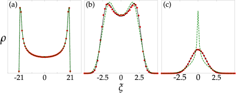
Figure 1: Calculation of the DOS, $\rho(\xi)$, of the Hamiltonian $H$ of (7) with $M=5000$ samples of $2000\times 2000$ matrices for (a) low, (b) moderate and (c) high noise ($\sigma/J$=0.1, 1 and 10 respectively with $\sigma=1$). For each figure we show the results of free convolution defined in Scheme I ($\rho^{\left(A_{1}\boxplus B_{1}\right)}$; black solid line), Scheme II ($\rho^{\left(A_{2}\boxplus B_{2}\right)}$; green dashed line) and exact diagonalization ($\rho^{\left(H\right)}$; red dotted line).

We observe that for Scheme I we have excellent agreement between $\rho^{\left(H\right)}$ and $\rho^{\left(A_{1}\boxplus B_{1}\right)}$ across all values of $\sigma/J$, which is evident from visual inspection; in contrast, Scheme II shows variable quality of fit.

We can understand the starkly different behaviors of the two partitioning schemes using the procedure outlined above to analyze the accuracy of the approximations $\rho^{\left(H\right)}\approx\rho^{\left(A_{1}\boxplus B_{1}\right)}$ and $\rho^{\left(H\right)}\approx\rho^{\left(A_{2}\boxplus B_{2}\right)}$. For Scheme I, we observe that the approximation (2) is of degree $k=8$; the discrepancy lies solely in the term $\left\langle\left(A_{1}B_{1}\right)^{4}\right\rangle$ Popescu (2011). Free probability expects this term to vanish, since both $A_{1}$ and $B_{1}$ are centered (i.e. $\left\langle A_{1}\right\rangle=\left\langle B_{1}\right\rangle=0$) and hence must satisfy (5b) with $n_{1}=m_{1}=\cdots=n_{4}=m_{4}=1$. In contrast, we can calculate its true value from the definitions of $A_{1}$ and $B_{1}$. By definition of the NET $\left\langle\cdot\right\rangle$, only closed paths contribute to the term. Hence, only two types of terms can contribute to $\left\langle\left(A_{1}B_{1}\right)^{4}\right\rangle$; these are expressed diagrammatically in Figure 2. The matrix $A_{1}$ weights each path by a factor of $h$, while $B_{1}$ weights each path by $J$, and in addition forces the path to hop to an adjacent site.

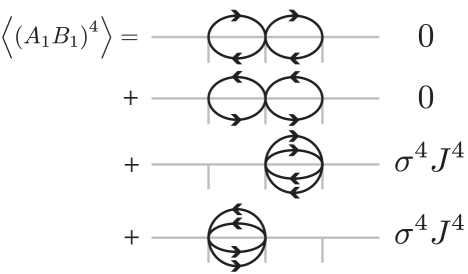
Figure 2: Diagrammatic expansion of the term $\left\langle A_{1}B_{1}A_{1}B_{1}A_{1}B_{1}A_{1}B_{1}\right\rangle$ in terms of allowed paths dictated by the matrix elements of $A_{1}$ and $B_{1}$ of Scheme I in (8a).

Consequently, we can write explicitly

$$\left\langle\left(A_{1}B_{1}\right)^{4}\right\rangle= \frac{1}{N}\sum_{i}\mathbb{E}\left(h_{i}Jh_{i-1}Jh_{i}Jh_{i+1}J\right)$$

$$+\frac{1}{N}\sum_{i}\mathbb{E}\left(h_{i}Jh_{i+1}Jh_{i}Jh_{i-1}J\right)$$

$$+\frac{1}{N}\sum_{i}\mathbb{E}\left(h_{i}Jh_{i-1}Jh_{i}Jh_{i-1}J\right)$$

$$+\frac{1}{N}\sum_{i}\mathbb{E}\left(h_{i}Jh_{i+1}Jh_{i}Jh_{i+1}J\right)$$

$$= 2J^{4}\mathbb{E}\left(h_{i}\right)^{2}\mathbb{E}\left(h_{i}^{2}\right)+2J^{4}\mathbb{E}\left(h_{i}^{2}\right)^{2}=0+2J^{4}\sigma^{4},$$ (10)

where the second equality follows from the independence of the $h_{i}$’s. As this is the only source of discrepancy at the eighth moment, this explains why the agreement between the free and exact PDFs is so good, as the leading order correction is in the eighth derivative of $\rho^{\left(A_{1}\boxplus B_{1}\right)}$ with coefficient $2\sigma^{4}J^{4}/8!=\left(\sigma J\right)^{4}/20160$. In contrast, we observe for Scheme II that the leading order correction is at $k=4$, where the discrepancy lies in $\left\langle A_{2}^{2}B_{2}^{2}\right\rangle$. Free probability expects this to be equal to $\left\langle A_{2}^{2}B_{2}^{2}\right\rangle=\left\langle A_{2}^{2}\right\rangle\left\langle B_{2}^{2}\right\rangle=\left\langle X^{2}\right\rangle^{2}=\left(J^{2}+\sigma^{2}/2\right)^{2}$, whereas the exact value of this term is $J^{2}\left(J^{2}+\sigma^{2}\right)$. Therefore the discrepancy is in the fourth derivative of $\rho^{\left(A\boxplus B\right)}$ with coefficient $\left(-\sigma^{4}/4\right)/4!=-\sigma^{4}/96$.

Analytic free convolution.—

Free probability allows us also to calculate the limiting distributions of $\rho^{\left(A\boxplus B\right)}$ in the macroscopic limit of infinite matrix sizes $N\rightarrow\infty$ and infinite samples $M\rightarrow\infty$. In this limit, the DOS $\rho^{\left(A\boxplus B\right)}$ is given as a particular type of integral convolution of $\rho^{\left(A\right)}$ and $\rho^{\left(B\right)}$. We now calculate the free convolution analytically in the macroscopic limit for the two partitioning schemes discussed above, thus sidestepping the cost of sampling and matrix diagonalization altogether.

The key tool to performing the free convolution analytically is the $R$-transform $r\left(w\right)=g^{-1}\left(w\right)-w^{-1}$ Voiculescu (1985), where $g^{-1}$ is defined implicitly via the Cauchy transform

$$w=\int_{\mathbb{R}}\frac{\rho\left(\xi\right)}{g^{-1}\left(w\right)-\xi}d\xi.$$ (11)

For freely independent $A$ and $B$, the $R$-transforms linearize the free convolution, i.e. $R^{\left(A\boxplus B\right)}\left(w\right)=R^{\left(A\right)}\left(w\right)+R^{\left(B\right)}\left(w\right)$, and that the PDF can be recovered from the Plemelj–Sokhotsky inversion formula by

$$\rho^{\left(A\boxplus B\right)}\left(\xi\right) =\frac{1}{\pi}\mbox{Im}\left(\left(g^{\left(A\boxplus B\right)}\right)^{-1}\left(\xi\right)\right)$$ (12a)

$$g^{\left(A\boxplus B\right)}\left(w\right) =R^{\left(A\boxplus B\right)}\left(w\right)+w^{-1}.$$ (12b)

As an example, we apply this to Scheme I with each iid $h_{i}$ following a Wigner semicircle distribution with PDF $p_{W}\left(\xi\right)=\sqrt{4-\xi^{2}}/4\pi$ on the interval $\left[-2,2\right]$. As described earlier (Using semicircular noise instead of Gaussian noise simplifies the analytic calculation considerably.) From the DOS $\rho^{\left(A_{1}\right)}=p_{W}$, we calculate its Cauchy transform (i.e. its retarded Green function)

$$G^{\left(A_{1}\right)}\left(z\right) =\lim_{\epsilon\downarrow 0}\int_{\mathbb{R}}\frac{\rho^{\left(A_{1}\right)}\left(\xi\right)}{z-\left(\xi+i\epsilon\right)}d\xi=\frac{z-\sqrt{z^{2}-4}}{2}.$$ (13)

Next, take the functional inverse

$$g^{\left(A_{1}\right)}\left(w\right)=\left(G^{\left(A_{1}\right)}\right)^{-1}\left(w\right)=w+\frac{1}{w}.$$ (14)

Subtracting $1/w$ finally yields the $R$-transform $r^{\left(A\right)}\left(w\right)=w$. Similarly with $\rho^{\left(B_{1}\right)}=p_{AS}$, we have its Cauchy transform

$$G^{\left(B_{1}\right)}\left(z\right)=\lim_{\epsilon\downarrow 0}\int_{\mathbb{R}}\frac{\rho^{\left(B_{1}\right)}\left(\xi\right)}{z-\left(\xi+i\epsilon\right)}d\xi=\frac{1}{\sqrt{z^{2}-4J^{2}}}$$ (15)

and its functional inverse

$$g^{\left(B_{1}\right)}\left(w\right)=\frac{\sqrt{1+4J^{2}w^{2}}}{w},$$ (16)

which finally yields the $R$-transform $R^{\left(B_{1}\right)}\left(w\right)=\left(-1+\sqrt{1+4J^{2}w^{2}}\right)/w$.

To perform the free convolution analytically, we add the $R$-transforms to get $R^{\left(A_{1}\boxplus B_{1}\right)}\left(w\right)=R^{\left(A_{1}\right)}\left(w\right)+R^{\left(B_{1}\right)}\left(w\right)$, from which we obtain

$$g^{\left(A_{1}\boxplus B_{1}\right)}\left(w\right)=w+\frac{\sqrt{1+4J^{2}w^{2}}}{w}.$$ (17)

The final steps are to calculate the functional inverse $\left(g^{\left(A_{1}\boxplus B_{1}\right)}\right)^{-1}$ and take its imaginary part to obtain $\rho^{\left(A_{1}\boxplus B_{1}\right)}$. Unfortunately, $\left(g^{\left(A_{1}\boxplus B_{1}\right)}\right)^{-1}$ cannot be written in a compact closed form; nevertheless, the inversion can be calculated numerically. We present calculations of the DOS as a function of noise strength $\sigma/J$ in Figure 3, showing again that the free convolution is an excellent approximation to the exact DOS.

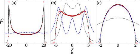
Figure 3: DOS, $\rho(\xi)$, of the Hamiltonian (7) with $M=5000$ samples of $2000\times 2000$ matrices with (a) low, (b) moderate and (c) high semicircular on-site noise ($\sigma/J$=0.1, 1 and 10 respectively with $\sigma=1$), as calculated with exact diagonalization (red dotted line), free convolution (black solid line), and perturbation theory with $A_{1}$ as reference (blue dashed line) and $B_{1}$ as reference (gray dash-dotted line). The partitioning scheme is Scheme I of (8a).

Comparison with other approximations.—

For comparative purposes, we also performed calculations using standard second-order matrix perturbation theory Horn and Johnson (1990) for both partitioning schemes. The results are also shown in Figure 3. Unsurprisingly, perturbation theory produces results that vary strongly with $\sigma/J$, and that the different series, based on whether $A$ is considered a perturbation of $B$ or vice versa, have different regimes of applicability. Furthermore it is clear even from visual inspection that the second moment of the DOS calculated using second-order perturbation theory is in general incorrect. In contrast, the free convolution produces results with a more uniform level of accuracy across the entire range of $\sigma/J$, and that we have at least the first three moments being correct Movassagh and Edelman .

It is also natural to ask what mean-field theory, another standard tool, would predict. Interestingly, the limiting behavior of Scheme I as $N\rightarrow\infty$ is equivalent to a form of mean-field theory known as the coherent potential approximation (CPA) Neu and Speicher (1994, 1995a, 1995b) in condensed matter physics, and is equivalent to the Blue’s function formalism in quantum chromodynamics for calculating one-particle irreducible self-energies Zee (1996). The breakdown in the CPA in the term $\left\langle\left(A_{1}B_{1}\right)^{4}\right\rangle$ is known Blackman et al. (1971); Thouless (1974); however, to our knowledge, the magnitude of the deviation was not explained. In contrast, our error analysis framework affords us such a quantitative explanation.

Finally, we discuss the predictions of isotropic entanglement theory, which proposes a linear interpolation between the classical convolution $\rho^{\left(A*B\right)}\left(\xi\right)=\int_{-\infty}^{\infty}\rho^{\left(A\right)}\left(\xi\right)\rho^{\left(B\right)}\left(x-\xi\right)dx$ and the free convolution $\rho^{\left(A\boxplus B\right)}\left(\xi\right)$ in the fourth cumulant Movassagh and Edelman ; Movassagh and Edelman (2011). The classical convolution can be calculated directly from the random matrices $A$ and $B$; by diagonalizing the matrices as $A=Q_{A}^{-1}\Lambda_{A}Q_{A}$ and $B=Q_{B}^{-1}\Lambda_{B}Q_{B}$, the classical convolution $\rho^{\left(A*B\right)}\left(\xi\right)$ can be computed from the eigenvalues of random matrices of the form $Z_{cl}=\Lambda_{A}+\Pi^{-1}\Lambda_{B}\Pi$ where $\Pi$ is a $N\times N$ random permutation matrix. It is instructive to compare this with the free convolution, which can be sampled from matrices of the form $Z^{\prime}=\Lambda_{A}+Q^{-1}\Lambda_{B}Q$, which can be shown by orthogonal invariance of the Haar measure random matrices $Q$ to be equivalent to sampling matrices of the form $Z=A+Q^{-1}BQ$ described previously.

As discussed previously, the lowest three moments of $Z$ and $H$ are identical; this turns out to be true also for $Z_{cl}$ Movassagh and Edelman . Therefore IE proposes to interpolate via the fourth cumulant, with interpolation parameter $p$ defined as

$$p=\frac{\kappa_{4}^{\left(H\right)}-\kappa_{4}^{\left(A\boxplus B\right)}}{\kappa_{4}^{\left(A*B\right)}-\kappa_{4}^{\left(A\boxplus B\right)}}$$ (18)

We observe that for Scheme I, IE appears to always favor the free convolution limit ($p=0$) as opposed to the classical limit ($p=1$); this is not surprising as we know from our previous analysis that $\kappa_{4}^{\left(H\right)}=\kappa_{4}^{\left(A_{1}\boxplus B_{1}\right)}$, and that the agreement with the exact diagonalization result is excellent regardless of $\sigma/J$. In Scheme II, however, we observe the unexpected result that $p$ is always negative and that the agreement varies with the noise strength $\sigma/J$. From the moment expansion we understand why; we have that the first three moments match while $\kappa_{4}^{\left(A_{2}+B_{2}\right)}-\kappa_{4}^{\left(A_{2}\boxplus B_{2}\right)}=-\sigma^{4}/4$. The discrepancy lies in the term $\left\langle A_{2}^{2}B_{2}^{2}\right\rangle$, which is expected to have the value $\left\langle A_{2}^{2}\right\rangle\left\langle B_{2}^{2}\right\rangle=\left(J^{2}+\sigma^{2}/2\right)^{2}$ in free probability but instead has the exact value $J^{2}\left(J^{2}+\sigma^{2}\right)$. Furthermore, we have that $\kappa_{4}^{\left(A_{2}*B_{2}\right)}\neq\kappa_{4}^{\left(A_{2}\boxplus B_{2}\right)}$where the only discrepancy lies is in the so-called departing term $\left\langle A_{2}B_{2}A_{2}B_{2}\right\rangle$ Movassagh and Edelman ; Movassagh and Edelman (2011). This term contributes 0 to $\kappa_{4}^{\left(A\boxplus B\right)}$ but has value $\left\langle A_{2}^{2}\right\rangle\left\langle B_{2}^{2}\right\rangle=\left(J^{2}+\sigma^{2}/2\right)^{2}$ in $\kappa_{4}^{\left(A_{2}*B_{2}\right)}$, since for the classical convolution we have that $\left\langle\Pi_{s=1}^{r}\left(A_{2}^{n_{s}}B_{2}^{m_{s}}\right)\right\rangle=\left\langle A_{2}^{\sum_{s=1}^{r}n_{s}}\right\rangle\left\langle B_{2}^{\sum_{s=1}^{r}m_{s}}\right\rangle$. This therefore explains why we observe a negative $p$, as this calculation shows that

$$p=\frac{\kappa_{4}^{\left(A_{2}+B_{2}\right)}-\kappa_{4}^{\left(A_{2}\boxplus B_{2}\right)}}{\kappa_{4}^{\left(A_{2}*B_{2}\right)}-\kappa_{4}^{\left(A_{2}\boxplus B_{2}\right)}}=-2\left(2\left(\frac{\sigma}{J}\right)^{-2}+1\right)^{-2}$$ (19)

which is manifestly negative.

In conclusion, we have demonstrated that the accuracy of approximations using the free convolution depend crucially on the particular choice of partitioning scheme for the Hamiltonian. We have found an unexpectedly accurate approximation for the DOS of disordered Hamiltonians, both for finite dimensional systems and in the macroscopic limit $N\rightarrow\infty$. In particular, this approximation remains accurate no matter the strength of noise present in the system. Our error analysis framework provides an explanation for this accuracy, namely that the lowest seven moments of the eigenvalues distribution are correct, with the first discrepancy only in one particular term arising at the eighth moment.

We expect our results to be generally applicable to arbitrary Hamiltonians, and are currently investigating the validity of these approximations for electronic structure models on two- and three-dimensional lattices. These results pave the way toward constructing even more accurate approximations using free probability, guided by a rigorous error analysis framework in terms of the accuracy of successive moments. Our results represent an optimistic beginning to the use of powerful and highly accurate nonperturbative methods for studying the electronic properties of disordered condensed matter systems regardless of the strength of noise present. We expect that these methods will be especially useful when the presence of noise is not merely a perturbation of a perfect system, but rather, crucial to the emergence of unique physical phenomena.