Preliminary lattice study of $\sigma$ meson decay width

Abstract

We report an exploratory lattice investigation of $\sigma$ meson decay width using $s$-wave scattering phase for isospin $I=0$ pion-pion ($\pi\pi$) system. Rummukainen-Gottlieb formula is used to estimate the scattering phase, which demonstrate the presence of a resonance around $\sigma$ meson. Using the effective range formula we extract the effective $\sigma\to\pi\pi$ coupling constant as $g_{\sigma\pi\pi}=2.69(44)$ GeV, which is consistent with theoretical predictions. The estimated decay width is about $236\pm 49$ MeV. These simulations are carried out on a $16^{3}\times 48$ MILC gauge configuration with the $N_{f}=2+1$ flavor of the “Asqtad” improved staggered dynamical sea quarks at $m_{\pi}/m_{\sigma}\approx 0.414$ and the lattice spacing $a\approx 0.15$ fm.

I Introduction

It is well-known that $\sigma$ meson is a resonance. In 2010, Particle Data Group (PDG) lists the meson $f_{0}(600)$, which is usually called $\sigma$ meson $I(J^{PC})=0(0^{++})$, with mass $400-1200$ MeV and width $600-1000$ MeV Nakamura:2010zzi . Its existence has been established by some refinements of the experimental analyses Ambrosino:2006hb ; Ablikim:2006bz ; Ablikim:2004qna ; Muramatsu:2002jp ; Aitala:2000xu ; Asner:1999kj ; Svec:1995xr and some phenomenological studies Oller:1997ti ; Hyodo:2010jp ; Mennessier:2010xg ; Caprini:2008fc ; Yndurain:2007qm ; Caprini:2005zr ; Escribano:2002iv ; Giacosa:2007bn ; Pelaez:2004xp . The Dalitz plot analysis of E791 Aitala:2000xu yields its decay width about $324$ MeV. Moreover, $\sigma$ meson has been extensively studied with BES data Ablikim:2006bz ; Ablikim:2004qna , and most recent analysis gives its pole position: $\sigma$ $(541\pm 39)+i(252\pm 42)$ MeV Ablikim:2006bz .

The direct determination of $\sigma$ resonance parameters from QCD is quite difficult because it is a nonperturbative problem. However, some theoretical efforts are still taken to investigate $\sigma$ meson and estimate its resonance parameters Oller:1997ti ; Hyodo:2010jp ; Mennessier:2010xg ; Caprini:2008fc ; Yndurain:2007qm ; Caprini:2005zr ; Escribano:2002iv ; Giacosa:2007bn ; Pelaez:2004xp . $\sigma$ meson was originally introduced to fit experimental data and its mass was chosen to reproduce the experimental results. There is a wide variety for defining its mass and width. Some authors use the pole approach with the mass and width of resonance taken from the position of the pole of the T-matrix Escribano:2002iv . Another way to study the mass and width of resonances is through the use of the spectral function Giacosa:2007bn , etc.

The most practicable method to nonperturbatively get $\sigma$ resonance parameters from first principles is using lattice QCD. To date, there is no report about lattice study on $\sigma$ resonance parameters, mainly because the reliable calculation of the rectangular and vacuum diagrams are extremely difficult. Encouraged by J. Nebreda and J. Pelaez’s theoretical investigations on $\sigma$ resonance Nebreda:2010wv , our previous studies on $\sigma$ mass Fu:2011zzh , $\pi\pi$ scattering length Fu:2011bz , $\pi K$ scattering length Fu:2011wc , and $\kappa$ meson decay width Fu:2011xw ; Fu:2011xz , here we explore $\sigma$ resonance parameters through lattice simulation.

In the current study, we extract $\sigma$ decay width using $s$-wave scattering phase shift of the $\pi\pi$ system for isospin $I=0$ channel in the moving frame (MF). The simulations are performed on a MILC lattice ensemble with the $2+1$ flavors of the Asqtad improved staggered dynamical sea quarks Bernard:2010fr ; Bazavov:2009bb . The meson masses extracted from our previous studies Fu:2011zzh gave $m_{\pi}/m_{\sigma}\approx 0.414$, and lattice parameters were determined by MILC Collaboration.

II Methods

II.1 Scattering phase

The $\sigma$ resonance decays into a pair of pions in the $s$-wave. In the elastic $\pi\pi$ scattering, the relativistic Breit-Wigner formula (RBWF) Nakamura:2010zzi can be expressed as

$$\tan\delta_{0}=\frac{\sqrt{s}\,\Gamma_{R}(s)}{m_{\sigma}^{2}-s},\quad s=E_{CM}^{2}.$$ (1)

where $E_{CM}$ is its center-of-mass (CM) energy of $\pi\pi$ system, $\delta_{0}$ is its $s$-wave scattering phase, and decay width $\Gamma_{R}(s)$ can be written by means of the effective $\sigma\rightarrow\pi\pi$ coupling constant $g_{\sigma\pi\pi}$ Nebreda:2010wv ,

$$\Gamma_{R}(s)=\frac{g^{2}_{\sigma\pi\pi}}{8\pi}\frac{p}{s},\quad p=\sqrt{\frac{s}{4}-m_{\pi}^{2}}.$$ (2)

By inspecting eqs. (1) and (2), an expression of the $s$-wave scattering phase with the invariant mass $\sqrt{s}$ is given by so-called effective range formula (ERF), namely,

$$\tan{\delta_{0}}=\frac{g^{2}_{\sigma\pi\pi}}{8\pi}\frac{p}{\sqrt{s}(m_{\sigma}^{2}-s)},$$ (3)

which enable us either a linear fit or solving for two unknown parameters: $g_{\sigma\pi\pi}$ and $m_{\sigma}$. Then $\sigma$ decay width $\Gamma_{\sigma}$ can be estimated through

$$\Gamma_{\sigma}=\Gamma_{R}(s)\Bigg{|}_{s=m_{\sigma}^{2}}=\frac{g^{2}_{\sigma\pi\pi}}{8\pi}\frac{p_{\sigma}}{m_{\sigma}^{2}},\quad p_{\sigma}=\sqrt{\frac{m_{\sigma}^{2}}{4}-m_{\pi}^{2}}.$$ (4)

Thus, equations (3) and (4) give us a way to obtain $m_{\sigma}$ and $\Gamma_{\sigma}$ through lattice simulation.

II.2 Finite size formula

In this work, we focus on $\sigma$ meson decay into a pair of pions in the $s$-wave, and only investigate the $\pi\pi$ system with isospin $(I,I_{z})=(0,0)$.

II.2.1 Center of mass frame

In the non-interacting case, the energy eigenvalues of $\pi\pi$ system are given by

$$E=2\sqrt{m_{\pi}^{2}+p^{2}},$$

where $p=|{\mathbf{p}}|,{\mathbf{p}}=(2\pi/L){\mathbf{n}}$, and ${\mathbf{n}}\in\mathbb{Z}^{3}$. For a typical lattice study, the energy for ${\mathbf{n}}\neq 0$ is much larger than sigma mass $m_{\sigma}$. For our case, the lowest energy for ${\mathbf{n}}\neq 0$ calculated from $m_{\pi}$ and $m_{\sigma}$ is $E=1.56\times m_{\sigma}$, which is obviously not eligible to study $\sigma$ meson. Thus, we can only consider ${\mathbf{n}}=0$ case, and the energy $E=0.828\times m_{\sigma}$, which is still a not good choice.

In the interacting case, the energy eigenvalues are moved by the hadronic interaction from $E$ to $\overline{E}$, and the energy eigenvalue for the $\pi\pi$ system is given by

$$\overline{E}=2\sqrt{m_{\pi}^{2}+k^{2}},\quad k=\frac{2\pi}{L}q,$$

where $q$ is not required to be an integer. In the CM frame these energy eigenvalues transform under the irreducible representation $\Gamma=T_{1}^{+}$ of the cubic group $O_{h}$. It is the famous Lüscher formula that relates the energy $\overline{E}$ to the scattering phase $\delta_{0}$ Luscher:1990ux ; Luscher:1990ck , namely,

$$\tan\delta_{0}(k) = \frac{\pi^{3/2}q}{\mathcal{Z}_{00}(1;q^{2})},$$ (5)

$$\mathcal{Z}_{00}(s;q^{2}) = \frac{1}{\sqrt{4\pi}}\sum_{{\mathbf{n}}\in\mathbb{Z}^{3}}\frac{1}{\left(|{\mathbf{n}}|^{2}-q^{2}\right)^{s}}.$$ (6)

The zeta function can be efficiently evaluated by the method in ref. Yamazaki:2004qb .

II.2.2 Moving frame

To make the energy of the $\pi\pi$ system is closer to sigma mass $m_{\sigma}$, we adopt the moving frame (MF) Rummukainen:1995vs with total momentum ${\mathbf{P}}=(2\pi/L){\mathbf{d}}$, ${\mathbf{d}}\in\mathbb{Z}^{3}$. For the non-interacting case its energy eigenstates are given by

$$E_{MF}=\sqrt{m_{\pi}^{2}+p_{1}^{2}}+\sqrt{m_{\pi}^{2}+p_{2}^{2}},$$

where $p_{1}=|{\mathbf{p}}_{1}|$,$p_{2}=|{\mathbf{p}}_{2}|$, and ${\mathbf{p}}_{1}$, ${\mathbf{p}}_{2}$ define three-momenta of two pions, respectively, which meet

$${\mathbf{p}}_{1}=\frac{2\pi}{L}{\mathbf{n}}_{1},\quad{\mathbf{p}}_{2}=\frac{2\pi}{L}{\mathbf{n}}_{2},\quad{\mathbf{n}}_{1},{\mathbf{n}}_{2}\in\mathbb{Z}^{3},\quad{\mathbf{P}}={\mathbf{p}}_{1}+{\mathbf{p}}_{2}.$$ (7)

In the MF, the CM is moving with a velocity of ${\mathbf{v}}={\mathbf{P}}/E_{MF}$. Using the Lorentz transformation with a boost factor $\gamma=1/\sqrt{1-{\mathbf{v}}^{2}}$, the $E_{CM}$ can be calculated by

$$E_{CM}=\gamma^{-1}E_{MF}=2\sqrt{m_{\pi}^{2}+p^{*2}},$$ (8)

where

$$p^{*}=|{\mathbf{p}}^{*}|\,,\quad{\mathbf{p}}^{*}={\mathbf{p}}^{*}_{1}=-{\mathbf{p}}^{*}_{2}=\frac{1}{2}\vec{\gamma}^{-1}({\mathbf{p}}_{1}-{\mathbf{p}}_{2}),$$ (9)

here and hereafter we denote the CM momenta with an asterisk $(^{\ast})$, the boost factor acts in the direction of ${\mathbf{v}}$, and we adopt the shorthand notation

$$\vec{\gamma}^{-1}{\mathbf{p}}=\gamma^{-1}{\mathbf{p}}_{\parallel}+{\mathbf{p}}_{\perp},$$ (10)

where ${\mathbf{p}}_{\parallel}$ and ${\mathbf{p}}_{\perp}$ are parallel and perpendicular components of ${\mathbf{p}}$. We note that the ${\mathbf{p}}^{*}$ are quantized as

$${\mathbf{p}}^{*}=\frac{2\pi}{L}{\mathbf{r}}\,,\quad{\mathbf{r}}\in P_{\mathbf{d}},$$ (11)

where

$$P_{\mathbf{d}}=\left\{{\mathbf{r}}\left|{\mathbf{r}}=\vec{\gamma}^{-1}\left({\mathbf{n}}+\frac{1}{2}{\mathbf{d}}\right),\right.\ {\mathbf{n}}\in\mathbb{Z}^{3}\right\}.$$ (12)

We are specially interest in one MF, which are one pion at rest, one pion with momentum ${\mathbf{p}}=(2\pi/L){\mathbf{e}}_{3}$ (${\mathbf{d}}={\mathbf{e}}_{3}$) and $\sigma$ meson with momentum ${\mathbf{P}}={\mathbf{p}}$. For our case, we found that its invariant mass takes $\sqrt{s}=0.994\times m_{\sigma}$, which is significantly closer to $m_{\sigma}$ than that in the CM frame. Thus, in this work we will only study this case.

In the interacting case, the $\overline{E}_{CM}$ is given by

$$\overline{E}_{CM}=2\sqrt{m_{\pi}^{2}+k^{2}},\quad k=\frac{2\pi}{L}q.$$ (13)

where $q$ is no longer an integer. In this work, we only use one MF with ${\mathbf{d}}={\mathbf{e}}_{3}$, where the energy eigenstates transform under the irreducible representation $A_{2}^{-}$ of the tetragonal group $D_{4h}$. We use the famous Rummukainen-Gottlieb formula to relate the energy eigenstates to the $\pi\pi$ scattering phase shift $\delta_{0}$, namely,

$$\tan\delta_{0}(k)=\frac{\gamma\pi^{3/2}q}{\mathcal{Z}_{00}^{\mathbf{d}}(1;q^{2})},$$ (14)

where we suppose that the higher phase shifts $\delta_{l}$ ($l=2,4,6,...$) are negligible, and the zeta function

$$Z_{00}^{{\mathbf{d}}}(s;q^{2})=\sum_{{\mathbf{r}}\in P_{\rm d}}\frac{1}{(|{\mathbf{r}}|^{2}-q^{2})^{s}},$$ (15)

here the set $P_{\mathbf{d}}$ is defined in eq. (12). $k$ is the scattering momentum defined through the invariant mass $\sqrt{s}$, namely, $\sqrt{s}=\sqrt{E_{MF}^{2}-p^{2}}=2\sqrt{m_{\pi}^{2}+k^{2}}$. The calculation method of $Z_{00}^{{\mathbf{d}}}(1;q^{2})$ is discussed in refs. Yamazaki:2004qb ; Fu:2011xw .

II.3 Correlation matrix

To evaluate the energy eigenstates, we build a matrix of the correlation function, namely,

$$C(t)=\left(\begin{array}[]{ll}\langle 0|{\cal O}_{\pi\pi}^{\dagger}(t){\cal O}_{\pi\pi}(0)|0\rangle&\langle 0|{\cal O}_{\pi\pi}^{\dagger}(t){\cal O}_{\sigma}(0)|0\rangle\vspace{0.3cm}\\ \langle 0|{\cal O}_{\sigma}^{\dagger}(t){\cal O}_{\pi\pi}(0)|0\rangle&\langle 0|{\cal O}_{\sigma}^{\dagger}(t){\cal O}_{\sigma}(0)|0\rangle\end{array}\right),$$ (16)

where ${\cal O}_{\sigma}(t)$ and ${\cal O}_{\pi\pi}(t)$ are interpolating operators for $\sigma$ meson and $\pi\pi$ system, respectively. These interpolating operators employed here are the same as in our previous studies Bernard:2007qf ; Fu:2011zzh ; Fu:2011zzl . However, to make this work self-contained, we will give the necessary definitions below.

II.3.1 $\pi\pi$ sector

Let us study $\pi\pi$ scattering of two Nambu-Goldstone pions in the Asqtad-improved staggered dynamical fermion formalism. Here we follow original derivations and notations in refs. Sharpe:1992pp ; Kuramashi:1993ka ; Fukugita:1994ve . Using operators ${\cal O}_{\pi}(x_{1})$, ${\cal O}_{\pi}(x_{2})$, ${\cal O}_{\pi}(x_{3})$, ${\cal O}_{\pi}(x_{4})$ for pions at points $x_{1}$, $x_{2}$, $x_{3}$ and $x_{4}$, respectively, with pion interpolating operators

$$\pi^{+}(t) = -\sum_{\mathbf{x}}\bar{d}(\mathbf{x},t)\gamma_{5}u(\mathbf{x},t),$$ (17)

$$\pi^{-}(t) = \sum_{\mathbf{x}}\bar{u}(\mathbf{x},t)\gamma_{5}d(\mathbf{x},t),$$ (18)

$$\pi^{0}(t) = \frac{1}{\sqrt{2}}\sum_{\mathbf{x}}[\bar{u}(\mathbf{x},t)\gamma_{5}u(\mathbf{x},t)-\bar{u}(\mathbf{x},t)\gamma_{5}d(\mathbf{x},t)],$$

we express the $\pi\pi$ four-point functions as

$$C_{\pi\pi}(x_{4},x_{3},x_{2},x_{1})=\bigl{<}{\cal O}_{\pi}(x_{4}){\cal O}_{\pi}(x_{3}){\cal O}_{\pi}^{{\dagger}}(x_{2}){\cal O}_{\pi}^{{\dagger}}(x_{1})\bigr{>}.$$

After summing over the spatial coordinates, we achieve the $\pi\pi$ four-point function with the momentum ${\mathbf{p}}$,

$$C_{\pi\pi}({\mathbf{p}},t_{4},t_{3},t_{2},t_{1}) = \sum_{\mathbf{x}_{1}}\sum_{\mathbf{x}_{2}}\sum_{\mathbf{x}_{3}}\sum_{\mathbf{x}_{4}}e^{i{\mathbf{p}}\cdot({\mathbf{x}}_{4}-{\mathbf{x}}_{2})}$$ (20)

$$\times C_{\pi\pi}(x_{4},x_{3},x_{2},x_{1}),$$

where $x_{1}\equiv(\mathbf{x}_{1},t_{1})$, $x_{2}\equiv(\mathbf{x}_{2},t_{2})$, $x_{3}\equiv(\mathbf{x}_{3},t_{3})$, $x_{4}\equiv(\mathbf{x}_{4},t_{4})$, and $t\equiv t_{3}-t_{1}$.

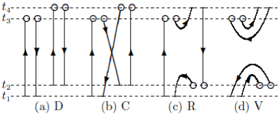
Figure 1: Diagrams contributing to $\pi\pi$ four-point functions. Short bars stand for wall sources. Open circles are sinks for local pion operators.

To avert the Fierz rearrangement of the quark lines Kuramashi:1993ka ; Fukugita:1994ve , we choose $t_{1}=0,t_{2}=1,t_{3}=t$, and $t_{4}=t+1$. We then construct the $\pi\pi$ operators for the $I=0$ channel as

$${\cal O}_{\pi\pi}^{I=0}(\mathbf{p},t) = \frac{1}{\sqrt{3}}\Bigl{\{}\pi^{-}(t)\pi^{+}(\mathbf{p},t+1)+\pi^{+}(t)\pi^{-}(\mathbf{p},t+1)$$ (22)

$$-\pi^{0}(t)\pi^{0}(\mathbf{p},t+1)\Bigl{\}}.$$

These operators belong to $A_{2}^{-}$ and the $(I,I_{z})=(0,0)$.

In the isospin limit, only four diagrams contribute to $\pi\pi$ scattering amplitudes Sharpe:1992pp ; Kuramashi:1993ka ; Fukugita:1994ve , which are plotted in figure 1, and labeled as direct($D$), crossed ($C$), rectangular ($R$), and vacuum ($V$) diagrams, respectively. It is well-known that the reliable evaluation of the rectangular ($R$) and vacuum diagrams ($V$) are extremely difficult. we tackle it by evaluating $T$ quark propagators Kuramashi:1993ka ; Fukugita:1994ve ; Fu:2011bz , namely, each propagator, which corresponds to a moving wall source at $t=0,\cdots,T-1$, are denoted by

$$\sum_{n^{\prime\prime}}D_{n^{\prime},n^{\prime\prime}}G_{t}(n^{\prime\prime})=\sum_{\mathbf{x}}\delta_{n^{\prime},({\mathbf{x}},t)},\quad 0\leq t\leq T-1.$$

The combination of $G_{t}(n)$ that we apply for $\pi\pi$ four-point functions is shown in figure 1. For the non-zero momentum, we used an up quark source with $1$, and an anti-up quark source with $e^{i{\mathbf{p}}\cdot{\mathbf{x}}}$ (except for $V$, where we use $1$) on each site for two pion creation operator, respectively. $D$, $C$, $R$ and $V$ are schematically shown in figure 1, and we can express them by means of the quark propagators $G$, namely,

$$C^{D}_{\pi\pi}({\mathbf{p}},t_{4},t_{3},t_{2},t_{1}) = \mbox{Re}\sum_{\mathbf{x}_{3},\mathbf{x}_{4}}e^{i{\mathbf{p}}\cdot{\mathbf{x}}_{4}}\left\langle\mbox{Tr}[G_{t_{1}}^{{\dagger}}({\mathbf{x}}_{3},t_{3})G_{t_{1}}({\mathbf{x}}_{3},t_{3})G_{t_{2}}^{{\dagger}}({\mathbf{x}}_{4},t_{4})G_{t_{2}}({\mathbf{x}}_{4},t_{4})]\right\rangle,$$ (23)

$$C^{C}_{\pi\pi}({\mathbf{p}},t_{4},t_{3},t_{2},t_{1}) = \mbox{Re}\sum_{\mathbf{x}_{3},\mathbf{x}_{4}}e^{i{\mathbf{p}}\cdot{\mathbf{x}}_{4}}\left\langle\mbox{Tr}[G_{t_{1}}^{{\dagger}}({\mathbf{x}}_{3},t_{3})G_{t_{2}}({\mathbf{x}}_{3},t_{3})G_{t_{2}}^{{\dagger}}({\mathbf{x}}_{4},t_{4})G_{t_{1}}({\mathbf{x}}_{4},t_{4})]\right\rangle,$$ (24)

$$C^{R}_{\pi\pi}({\mathbf{p}},t_{4},t_{3},t_{2},t_{1}) = \mbox{Re}\sum_{\mathbf{x}_{2},\mathbf{x}_{3}}e^{i{\mathbf{p}}\cdot{\mathbf{x}}_{2}}\left\langle\mbox{Tr}[G_{t_{1}}^{{\dagger}}({\mathbf{x}}_{2},t_{2})G_{t_{4}}({\mathbf{x}}_{2},t_{2})G_{t_{4}}^{{\dagger}}({\mathbf{x}}_{3},t_{3})G_{t_{1}}({\mathbf{x}}_{3},t_{3})]\right\rangle,$$ (25)

$$C_{\pi\pi}^{V}({\mathbf{p}},t_{4},t_{3},t_{2},t_{1}) = \mbox{Re}\sum_{\mathbf{x}_{2},\mathbf{x}_{3}}e^{i{\mathbf{p}}\cdot({\mathbf{x}}_{2}-{\mathbf{x}}_{3})}\left\langle\mbox{Tr}[G_{t_{1}}^{{\dagger}}(\mathbf{x}_{2},t_{2})G_{t_{1}}(\mathbf{x}_{2},t_{2})G_{t_{4}}^{{\dagger}}(\mathbf{x}_{3},t_{3})G_{t_{4}}(\mathbf{x}_{3},t_{3})]\right\rangle.$$ (26)

From our previous studies Fu:2011zzh ; Bernard:2007qf ; Fu:2011zzl , we found that when we calculate the disconnected part of the sigma correlator with non-zero momenta, the subtraction of the vacuum expectation value is not needed. Similarly, the vacuum diagram here is not accompanied by a vacuum subtraction for the cases with non-zero momenta.

As discussed in refs. Kuramashi:1993ka ; Fukugita:1994ve , the rectangular and vacuum diagrams create gauge-variant noise, which are reduced by performing the gauge field average without gauge fixing in this work. All four diagrams in figure 1 are required to study $\pi\pi$ scattering in the $I=0$ channel. As investigated in ref. Kuramashi:1993ka ; Fukugita:1994ve , in the isospin limit, the $\pi\pi$ correlator for the $I=0$ channel can be written with the combinations of four diagrams, namely,

$$C_{\pi\pi}(t)\equiv\left\langle{\cal O}_{\pi\pi}(t)|{\cal O}_{\pi\pi}(0)\right\rangle=D+\frac{1}{2}C-3R+\frac{3}{2}V,$$ (27)

where the operator ${\cal O}_{\pi\pi}$ denoted in eq. (22) creates a $\pi\pi$ state with the total isospin $0$. In practice we also evaluate the ratios

$$R^{X}(t)=\frac{C_{\pi\pi}^{X}({\mathbf{p}},0,1,t,t+1)}{C_{\pi}({\mathbf{0}},0,t)C_{\pi}({\mathbf{p}},1,t+1)},\hskip 7.11317ptX=D,C,R,\ {\rm and}\ V,$$ (28)

where $C_{\pi}({\mathbf{0}},0,t)$ and $C_{\pi}({\mathbf{p}},1,t+1)$ are the two-point pion correlators with the momentum ${\mathbf{0}}$ and ${\mathbf{p}}$, respectively.

We should bear in mind that, the contributions of non-Nambu-Goldstone pions in the intermediate states is exponentially suppressed for large $t$ due to its heavier masses compared to these of the Nambu-Goldstone pion Sharpe:1992pp ; Kuramashi:1993ka ; Fukugita:1994ve . Hence, we think that $\pi\pi$ interpolator does not greatly couple to other $\pi\pi$ tastes, and neglect this systematic errors.

II.3.2 $\sigma$ sector

In our previous studies Fu:2011zzh ; Bernard:2007qf ; Fu:2011zzl , we give a detailed procedure to evaluate $\langle 0|\sigma^{\dagger}(t)\sigma(0)|0\rangle$ . To simulate the correct number of quark species, we use an interpolation operator with the isospin $I=0$ and $J^{P}=0^{+}$ at source and sink,

$${\cal O}(x)\equiv\sum_{a,g}\frac{\bar{u}^{a}_{g}(x)u^{a}_{g}(x)+\bar{d}^{a}_{g}(x)d^{a}_{g}(x)}{\sqrt{2n_{r}}},$$

where $g$ is the index of the taste replica, $n_{r}$ is the number of the taste replicas, $a$ is the color index. After performing the Wick contractions of fermion fields, and summing over the taste index, for the light quark Dirac operator $M$, we obtain the time slice correlator $C(t)$ with the momentum ${\bf p}$

$$C(\mathbf{p},t) = -\frac{1}{2}\sum_{\mathbf{x}}e^{i\mathbf{p}\cdot\mathbf{x}}\langle\mbox{Tr}M^{-1}(\mathbf{x},t;\mathbf{x},t)\mbox{Tr}M^{-1}({\bf 0},0;{\bf 0},0)\rangle$$

$$+ \sum_{\mathbf{x}}(-)^{x}e^{i\mathbf{p}\cdot\mathbf{x}}\langle\mbox{Tr}[M^{-1}(\mathbf{x},t;{\bf 0},0)M^{-1^{\dagger}}\mathbf{x},t;{\bf 0},0)]\rangle,$$

where the first and second terms are the quark-line disconnected and connected contributions, respectively Fu:2011zzh ; Bernard:2007qf ; Fu:2011zzl . For the staggered quarks, the meson propagators behave as

$${\cal C}(t)=\sum_{i}A_{i}e^{-m_{i}t}+\sum_{i}A_{i}^{\prime}(-1)^{t}e^{-m_{i}^{\prime}t}+(t\rightarrow N_{t}-t),$$ (30)

where the oscillating term is a particle with opposite parity. For $\sigma$ correlator, we take only one mass with each parity in eq. (30) Fu:2011zzh ; Bernard:2007qf ; Fu:2011zzl . Thus, the $\sigma$ correlator was then fit to

$$C_{\sigma}(t)=b_{\sigma}e^{-m_{\sigma}t}+b_{\eta_{A}}(-)^{t}e^{-M_{\eta_{A}}t}+(t\rightarrow N_{t}-t),$$ (31)

where $b_{\eta_{A}}$ and $b_{\sigma}$ are two overlap factors.

II.3.3 Off-diagonal sector

To avoid the Fierz rearrangement of the quark lines, we choose $t_{1}=0,t_{2}=1$, and $t_{3}=t$ for the $\pi\pi\to\sigma$ three-point function, and choose $t_{1}=0,t_{2}=t$, and $t_{3}=t+1$ for the $\sigma\to\pi\pi$ three-point function Fukugita:1994ve .

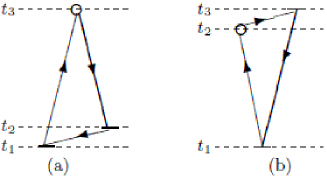
Figure 2: Diagrams contributing to $\pi\pi\to\sigma$ and $\sigma\to\pi\pi$. Short bars represent the wall sources. Open circles stand for the sinks of local pion operator. (a) Quark line contractions of $\pi\pi\to\sigma$ and (b) Quark line contractions of $\sigma\to\pi\pi$.

The quark line diagrams contributing to $\pi\pi\to\sigma$ and $\sigma\to\pi\pi$ three-point functions are plotted in figure 2(a) and figure 2(b), respectively. The $\pi\pi\to\sigma$ three-point function can be easily evaluated. However, the calculation of the $\sigma\to\pi\pi$ three-point function is quite difficult. For non-zero momenta, we adopted an up quark source with $1$, and an anti-up quark source with $e^{i{\mathbf{p}}\cdot{\mathbf{x}}}$ on each site for pion creation operator. The $\sigma\to\pi\pi$ and $\pi\pi\to\sigma$ three-point functions are schematically displayed in figure 1, and we can write them using quark propagators $G$, namely,

$$C_{\pi\pi\to\sigma}({\mathbf{p}},t_{3},t_{2},t_{1}) =$$ (33)

$$\mbox{Re}\sum_{{\mathbf{x}}_{3},{\mathbf{x}}_{1}}e^{i{\mathbf{p}}\cdot{\mathbf{x}}_{3}}\left\langle\mbox{Tr}[G_{t_{1}}({\mathbf{x}}_{3},t_{3})G_{t_{2}}^{{\dagger}}({\mathbf{x}}_{3},t_{3})G_{t_{2}}^{{\dagger}}({\mathbf{x}}_{1},t_{1})]\right\rangle,$$

$$C_{\sigma\to\pi\pi}({\mathbf{p}},t_{3},t_{2},t_{1}) =$$ (35)

$$\mbox{Re}\sum_{{\mathbf{x}}_{2},{\mathbf{x}}_{1}}e^{i{\mathbf{p}}\cdot{\mathbf{x}}_{2}}\left\langle\mbox{Tr}[G_{t_{1}}({\mathbf{x}}_{2},t_{2})G_{t_{3}}^{{\dagger}}({\mathbf{x}}_{2},t_{2})G_{t_{3}}^{{\dagger}}({\mathbf{x}}_{1},t_{1})]\right\rangle,$$

II.4 Extraction of energies

To map out “avoided level crossings” between $\sigma$ resonance and its decay products, we separate the ground state from first excited state by calculating the matrix of correlation function $C(t)$ in eq. (16). To extract two lowest energy eigenvalues, we utilize the variational method Luscher:1990ck and build a ratio of correlation function matrices as

$$M(t,t_{R})=C(t)\,C^{-1}(t_{R}),$$ (36)

with some reference time slice $t_{R}$ Luscher:1990ck . The two lowest energy states can be extracted through a fit to two eigenvalues $\lambda_{n}(t,t_{R})$ ($n=1,2$) of matrix $M(t,t_{R})$. Since we work on the staggered fermion, $\lambda_{n}(t,t_{R})$ ($n=1,2$) explicitly has an oscillating term Fu:2011xw ; Mihaly:1997 , namely,

$$\lambda_{n}(t,t_{R}) = A_{n}\cosh\left[-E_{n}\left(t-\frac{T}{2}\right)\right]$$ (38)

$$+(-1)^{t}B_{n}\cosh\left[-E_{n}^{\prime}\left(t-\frac{T}{2}\right)\right],$$

for a large $t$, which mean $0\ll t_{R}<t\ll T/2$ to suppress both the excited states and wrap-around contributions Feng:2009ij . Here we assume $\lambda_{1}(t,t_{R})>\lambda_{2}(t,t_{R})$.

III Lattice calculation

We used MILC lattice with $2+1$ dynamical flavors of Asqtad-improved staggered dynamical fermions. We worked on a $0.15$ fm lattice ensemble of $360$ $16^{3}\times 48$ gauge configurations with bare quark masses $am_{ud}/am_{s}=0.0097/0.0484$ and bare gauge coupling $10/g^{2}=6.572$. The lattice extent $L$ is about $2.5{\mathrm{f}m}$, the $u$ and $d$ quark masses are degenerate and the lattice spacing $a^{-1}=1.358^{+35}_{-13}$ GeV Bernard:2010fr ; Bazavov:2009bb .

We use the standard conjugate gradient method to obtain the required matrix element of the inverse fermion matrix. Periodic boundary condition is imposed to three spatial directions and temporal direction. We compute the propagators on all the time slices for the $\pi\pi$ correlation functions,. After averaging the correlator over all $48$ possible values, the statistics are greatly improved since we can put pion source at all possible time slices.

We calculate the off-diagonal correlator $C_{21}(t)$ by

$$C_{21}(t)=\frac{1}{T}\sum_{t_{s}}\left\langle\sigma(t+t_{s})(\pi\pi)^{\dagger}(t_{s})\right\rangle,$$

where we sum the correlator over all time slices and average it. Using the relation $C_{12}(t)=C_{21}^{\ast}(t)$, we obtain another off-diagonal correlator $C_{12}(t)$ for free Aoki:2007rd .

For the $\sigma$ correlator, $C_{22}(t)$, we can use the available propagators in Fu:2011zzh to build the $\sigma$ correlator

$$C_{22}(t)=\frac{1}{T}\sum_{t_{s}}\left\langle\sigma^{\dagger}(t+t_{s})\sigma(t_{s})\right\rangle,$$

where, again, we average all the possible correlators. One thing we must stress is that we use the $Z_{2}$ noisy estimators based on the random color fields to measure the disconnected contribution of the sigma correlator Fu:2006uw . In our previous work Fu:2006uw , we have presented the detailed procedures for the implementation of the $Z_{2}$ method. Using the standard discussed in ref. Muroya:2001yp , we determine that $1000$ noise $Z_{2}$ sources are sufficiently reliable to measure the disconnected part.

We also measure two-point pion correlators, namely,

$$C_{\pi}(t;{\mathbf{0}}) = \langle 0|\pi^{\dagger}({\mathbf{0}},t)\pi({\mathbf{0}},0)|0\rangle,$$ (39)

$$C_{\pi}(t;{\mathbf{p}}) = \langle 0|\pi^{\dagger}({\mathbf{p}},t)\pi({\mathbf{p}},0)|0\rangle,$$ (40)

where the $C_{\pi}(t;{\mathbf{0}})$ and $C_{\pi}(t;{\mathbf{p}})$ are correlators for the pion with the momentum ${\mathbf{0}}$ and ${\mathbf{p}}$, respectively.

IV Simulation results

IV.1 Time correlation function

In figure 3 the individual ratios, $R^{X}$ ($X=D,C$, $R$ and $V$)  are plotted as the functions of $t$. It is quite noisy for the disconnected diagram ($V$), but we can still get a signal up until time separation $t\sim 14$. Clear signals observed up until $t\sim 20$ for the rectangular amplitude and up until $t\sim 14$ for the vacuum amplitude show that the technique with the moving wall source without gauge fixing used in this paper is practically applicable.

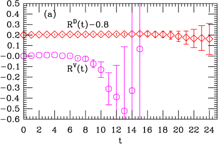
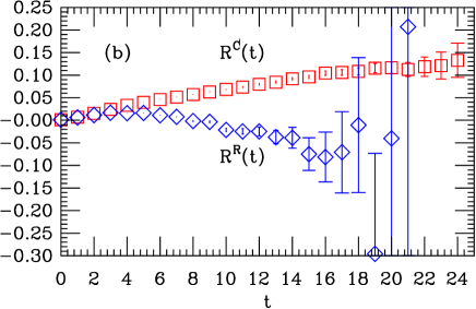
Figure 3: Individual amplitude ratios $R^{X}(t)$ for $\pi\pi$ four-point function as functions of $t$. (a) Direct diagram shifted by $0.8$ (red diamonds) and vacuum diagram (magenta octagons); (b) crossed (red squares) and rectangular (blue diamonds) diagrams.

The values of the direct amplitude $R^{D}$ is quite close to unity, indicating a weak interaction in this channel. The crossed amplitude increases linearly, implying a repulsion in this channel. After an beginning increase up to $t\sim 4$, the rectangular amplitude shows a approximately linear decrease up untill $t\sim 15$, suggesting an attractive force between two pions. We can note that the crossed and rectangular amplitudes own the same value at $t=0$. These features are what we expect Sharpe:1992pp .

The vacuum amplitude is quite small up until $t\sim 8-14$, and loss of the signals after that. This characteristic is in agreement with the Okubo-Zweig-Iizuka (OZI) rule and $\chi$PT in leading order, which predicts the vanishing of the vacuum amplitude Kuramashi:1993ka .

In figure 4, we display the real parts of the diagonal components ($\pi\pi\to\pi\pi$ and $\sigma\to\sigma$) and the off-diagonal component $\pi\pi\to\sigma$ for the correlation function $C(t)$.

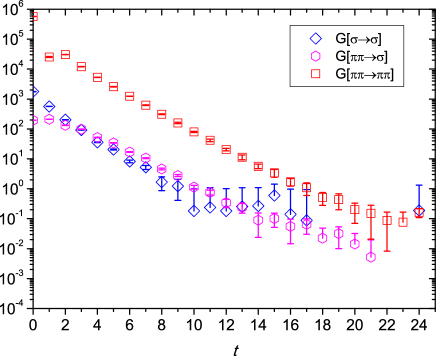
Figure 4: Real parts of the diagonal components ($\pi\pi\to\pi\pi$ and $\sigma\to\sigma$) and the off-diagonal component $\pi\pi\to\sigma$. Occasional points with negative central values for the off-diagonal component $\pi\pi\to\sigma$ and the diagonal component $\sigma\to\sigma$ are not displayed.

As we discussed in Fu:2011zzh ; Bernard:2007qf ; Fu:2011zzl , there exists the bubble contribution in sigma correlator, thus we will compute the scattering phase shift with the bubble term deducted from the sigma correlator. In Refs. Bernard:2007qf ; Fu:2011zzl , we parameterized the bubble term by three low-energy coupling constants which were fixed to our previous determined values Fu:2011zzh ; Fu:2011zzl in our concrete calculation. After removing the bubble term, the remaining sigma correlator has the clean information for sigma meson.

We calculate two eigenvalues $\lambda_{n}(t,t_{R})$ ($n=1,2$) for the matrix $M(t,t_{R})$ in eq. (36) with the reference time $t_{R}$. In figure 5, we plot our lattice results for $\lambda_{n}(t,t_{R})(n=1,2)$ as a function of time $t$ together with a correlated fit using eq. (38). From these fits we can extract the energies which will be used to obtain the scattering phase.

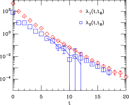
Figure 5: The eigenvalues $\lambda_{1}(t,t_{R})$ and $\lambda_{2}(t,t_{R})$ as the function of $t$. The solid lines are correlated fits to eq. (38). Occasional points with negative values in $\lambda_{2}(t,t_{R})$ are not shown.

To achieve the energies reliably, we should take two systematic errors into considerations: the excited states and the warp-around effects Feng:2010es . By denoting a fitting range $[t_{\mathrm{min}},t_{\mathrm{max}}]$ and changing $t_{\mathrm{min}}$ values and $t_{\mathrm{max}}$ numbers, we can suppress these systematic errors. In our concrete calculation, we take $t_{\mathrm{min}}=t_{R}+1$ and increase $t_{R}$ to restrain the excited state contributions Feng:2010es . Moreover, we select $t_{\mathrm{max}}$ to be enough aloof from the time slice $T/2$ to avert the warp-around contributions Feng:2010es . The fitting parameters $t_{R}$, $t_{\mathrm{min}}$ and $t_{\mathrm{max}}$, fit quality $\chi^{2}/\mathrm{dof}$ together with the fit results for $\overline{E}_{n}$ ($n=1,2$) are summarized in table 1.

Table 1: The values of the energy eigenvalues for the ground state ($n=1$) and first excited state ($n=2$). In table we list the reference time $t_{R}$, fitting range: $t_{\mathrm{min}}$ and $t_{\mathrm{max}}$, fit quality $\chi^{2}/\mathrm{dof}$ and fit values for $\overline{E}_{n}$ ($n=1,2$) in lattice units.

n	$t_{R}$	$t_{\mathrm{min}}$	$t_{\mathrm{max}}$	$a\overline{E}_{n}$	$\chi^{2}/\mathrm{dof}$
$1$	$6$	$7$	$12$	$0.6767(20)$	$0.922/2$
$2$	$5$	$6$	$12$	$0.8086(75)$	$0.158/3$

The mass $m_{\pi}$ and energy $E_{\pi}$ are achieved by a one-pole fit to $C_{\pi}(t;{\mathbf{0}})$ and $C_{\pi}(t;{\mathbf{p}})$ in eq. (40), respectively. Then the energy of the free pions $E_{1}^{0}$ take as $E_{1}^{0}=m_{\pi}+E_{\pi}$. These results are summarized in table 2 in lattice units. We note that $\overline{E}_{1}<E_{1}^{0}<\overline{E}_{2}$, which indicates a resonance existing in between.

Table 2: Summary of the energy $\overline{E}_{n}$ and the scattering phase shift $\delta$. The invariant mass $\sqrt{s}$, the momentum $k$ and the phase shifts $\delta$ calculated with eq. (41) are referred to as Cont, and those obtained with eq. (43) are referred to as Lat. The scattering momentum $k_{0}$ is calculated by $k_{0}^{2}=s/4-m_{\pi}^{2}$.

	$n=1$		$n=2$
$E^{0}_{n}$	$0.7085(6)$		—–
$\overline{E}_{n}$	$0.6767(20)$		$0.8086(38)$
	Cont	Lat	Cont	Lat
$\sqrt{s}$	$0.5511(25)$	$0.5613(25)$	$0.7068(43)$	$0.7179(44)$
$k^{2}$	$0.0155(7)$	$0.0185(8)$	$0.0644(15)$	$0.0699(17)$
$k_{0}^{2}$	—–	$0.0182(7)$	—–	$0.0684(16)$
$\tan\delta$	$0.380(17)$	$0.257(14)$	$-1.261(44)$	$-1.509(55)$
$\sin^{2}\delta$	$0.126(9)$	$0.0621(64)$	$0.614(16)$	$0.695(15)$

In table 3 we give the pion mass and its the energy with the momentum ${\mathbf{p}}=(2\pi/L){\mathbf{e}}_{3}$, calculated from the pion correlator. Also we show the sigma mass and its the energy with the same momentum, calculated from the $\sigma$ correlator.

Table 3: The mass $m$ of the $\pi$ and $\sigma$ meson, and the energy $E$ of the $\pi$ and $\sigma$ meson with momentum ${\mathbf{p}}=(2\pi/L){\mathbf{e}}_{3}$ in lattice units.

	$\pi$	$\sigma$
$am$	$0.2459(2)$	$0.594(35)$
$aE$	$0.4626(5)$	$0.714(22)$

IV.2 Lattice discretization effects

We should premeditate the discretization error in Rummukainen-Gottlieb formula (14). It comes from the Lorentz transformation from the MF to the CM frame. In Lorentz transformation we use,

$$\sqrt{s}=\sqrt{E_{MF}^{2}-p^{2}},\quad k^{2}=\frac{s}{4}-m_{\pi}^{2}.$$ (41)

On the lattice, Rummukainen and Gottlieb Rummukainen:1995vs suggest using the lattice modified relations,

$$\cosh(\sqrt{s}) = \cosh(E_{MF})-2\sin^{2}(p/2),$$ (42)

$$2\sin^{2}(k/2) = \cosh\left(\frac{\sqrt{s}}{2}\right)-\cosh(m_{\pi}).$$ (43)

To comprehend the discretization effects, we calculate invariant mass $\sqrt{s}$ and momentum $k$ from the relations both in the continuum (41) and on the lattice (43), and then calculate the phase shift. We regard the difference stemming from two choices as the discretization error. The results for the invariant mass $\sqrt{s}$, momentum $k$ and phase shift $\delta$ are tabled in table 2 in lattice units.

IV.3 Extraction of resonance parameters

From table 2, the differences due to the choice of the energy-momentum relations are obviously observed in $\sqrt{s}$ and $k$ . Moreover, the difference for phase shift $\delta$ is significantly larger than the statistical errors. These are also shown in figure 6, where the phase shift $\sin^{2}\delta$ is drawn and the abscissa is in lattice units. In table 2 we see that the sign of the phase shift $\delta$ at $\sqrt{s}<m_{\sigma}$ ($am_{\sigma}=0.594(33)$) is positive, and that at $\sqrt{s}>m_{\sigma}$ is negative. These features confirm the presence of a resonance around $\sigma$ mass.

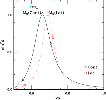
Figure 6: Scattering phase shift $\sin^{2}\delta$, positions of $m_{\sigma}$ and resonance mass $M_{R}$ are displayed. Cont refer to the results achieved with (41) and Lat to those with (43). The two lines are taken by eq. (44) with parameters $g_{\sigma\pi\pi}$ and $M_{R}$ obtained in eq. (47) and eq. (50), respectively.

In practice, we should extract the $\sigma$ meson decay width by fitting the phase shift data with the RBWF since the kinematic factors in the decay width depend explicitly on the quark mass Nebreda:2010wv . However, in this work, we just measured a lattice data on a set of quark mass, so we must take an alternative approach. As we discussed in section II.1, we parameterize the resonant characteristic of the $\delta_{0}$ using the effective $\sigma\to\pi\pi$ coupling constant $g_{\sigma\pi\pi}$, namely,

$$\tan\delta_{0}=\frac{g_{\sigma\pi\pi}^{2}}{8\pi}\frac{k}{\sqrt{s}(M_{R}^{2}-s)},$$ (44)

where $M_{R}$ is the resonance mass.

According to the discussions in ref. Nebreda:2010wv , we can reasonably assume that the coupling constant $g_{\sigma\pi\pi}$ is a constant since it changes quite slowly as the quark mass varies. Thus, equation (44) allows us to solve for two unknown parameters: the coupling constant $g_{\sigma\pi\pi}$, and resonance mass $m_{R}$. The discretization error may arise from the choice of $\sqrt{s}$ and $k$. Fortunately, our lattice results show that this does not cause a serious problem numerically. In table 2 we present the momentum $k_{0}$ evaluated by $k_{0}^{2}=s/4-m_{\pi}^{2}$. We notice that the difference between $k$ and $k_{0}$ is not considerable. Thus, we can ignore this systemic error for the current study. Actually, we use the momentum $k_{0}$ when applying eq. (44).

The coupling constant $g_{\sigma\pi\pi}$ and the resonance mass $M_{R}$ solved by eq. (44) read

$$g_{\sigma\pi\pi} = 3.22(52)\,{\rm GeV},$$ (45)

$$M_{R} = 0.660(31),$$ (46)

$$M_{R}/m_{\sigma} = 1.112(85),$$ (47)

where we utilize the eq. (41). If we employ the eq. (43), we achieve

$$g_{\sigma\pi\pi} = 2.69(44)\,{\rm GeV},$$ (48)

$$M_{R} = 0.691(37),$$ (49)

$$M_{R}/m_{\sigma} = 1.163(93).$$ (50)

The value of the coupling constant $g_{\sigma\pi\pi}$ is in reasonable agreement with $g_{\sigma\pi\pi}=2.47(45)\,{\rm GeV}$ obtained in ref. Kaminski:2009qg , $g_{\sigma\pi\pi}=2.97(4)\,{\rm GeV}$ Oller:2003vf and $g_{\sigma\pi\pi}=2.86\,{\rm GeV}$ Nebreda:2010wv .

In figure 6, we display the curves for $\sin^{2}\delta_{0}$ solved by eq. (44) with the coupling constant $g_{\sigma\pi\pi}$ and the resonance mass $M_{R}$ given in eq. (47) and eq. (50), respectively. The position of the resonance mass $M_{R}$ (at $\sin^{2}\delta_{0}=1$) are also displayed in figure 6 for two cases (black cross and red plus for the continuum and lattice cases, respectively). For visualized comparison, we also draw the sigma mass $m_{\sigma}$ (fancy cyan plus), which is in reasonable agreement with the $m_{R}$.

Supposing that the quark dependence of $g_{\sigma\pi\pi}$ is quite small Nebreda:2010wv , we can roughly calculate $\sigma$ meson decay width at the physical point as

$$\Gamma^{\rm phy}=\frac{g_{\sigma\pi\pi}^{2}}{8\pi}\frac{k^{\rm phy}}{(m_{\sigma}^{\rm phy})^{2}},$$

where $m_{\sigma}^{\rm phy}=513\pm 32$ MeV is the estimated physical $\sigma$ meson mass taken from PDG Nakamura:2010zzi , and momentum $k^{\rm phy}$ is calculated by

$$(k^{\rm phy})^{2}=\frac{(m_{\sigma}^{\rm phy})^{2}}{4}-(m_{\pi}^{\rm phy})^{2},$$

where $m_{\pi}^{\rm phy}$ is physical pion mass ($m_{\pi}^{\rm phy}\approx 140$ MeV) Nakamura:2010zzi . This produces

$$\Gamma^{\rm phy}=(337\pm 82)\,{\rm MeV}\,$$ (51)

where we use the data given in eq. (47), and

$$\Gamma^{\rm phy}=(236\pm 49)\,{\rm MeV}$$ (52)

where we employ the data given in eq. (50). We can observe that the difference stemming from two choices of the energy-momentum relations is larger than with the statistical error. Although our preliminary estimates for the $\sigma\to\pi\pi$ decay width in this work is not within the PDG estimated result $\Gamma=600-1000$MeV Nakamura:2010zzi , this is still an inspiring result, considering that we make a big assumption about the coupling constant does not depend on the quark mass, an perform a long chiral extrapolation, etc.

In the present study, we make an extensive use of the RBWF. It is well-known that the sigma meson is a very wide object and the RBWF approximation holds perfectly for relatively narrower objects. As discussed in ref. Doring:2011vk , we should adopt a much more model-independent approach to the extraction of the finite volume limit. In refs. Doring:2011nd ; Roca:2012rx ; Chen:2012rp , Oset et al. pointed out that if we have got three energies in the cubic box, with the momentum $p=0$ and $p$ different of zero, we can still use the finite volume formulas to get the phase shifts in a correct manner. Alternative methods are also discussed in these references. In our future tasks, we must address the phenomenological treatment.

V Conclusions

In this work, we have carried out a lattice calculation of the $s$-wave $\pi\pi$ scattering phase shift for isospin $I=0$ channel near $\sigma$-meson resonance with total non-zero momentum in one MF, for MILC “medium” coarse ($a=0.15$ fm) lattice ensemble. We employed the technique in refs. Kuramashi:1993ka ; Fukugita:1994ve , namely, the moving wall source without gauge fixing for the $I=0$ channel to obtain the reliable precision.

We have demonstrated that the phase shift data clearly shows the presence of a resonance at a mass around $\sigma$ meson mass. Moreover, we extracted $\sigma$ meson decay width from the phase shift data and showed that it is fairly compared with the corresponding PDG estimation Nakamura:2010zzi .

We adopted the ERF, which allows us to use the effective $\sigma\to\pi\pi$ coupling constant $g_{\sigma\pi\pi}$ to extrapolate our lattice simulation point $m_{\pi}/m_{\sigma}\approx 0.414$ to the physical point $m_{\pi}/m_{\sigma}\approx 0.273$, assuming that $g_{\sigma\pi\pi}$ is independent of quark mass. This is just a rough estimation. We are planning to improve it.

When our preliminary lattice results reported here are compared with its PDG quantities, it is clear that the lattice simulations is just rough estimation, and even can not be considered to be“physical” one. So we view our rudimentary works presented here as stepping out a first step to the study of $\sigma$ resonance from lattice QCD.

References

- (1) K. Nakamura et al. [ Particle Data Group Collaboration ], J. Phys. G 37 (2010) 075021.
- (2) F. Ambrosino et al. [KLOE Collaboration], at with the KLOE detector, Eur. Phys. J. C 49 (2007) 473 [arXiv:hep-ex/0609009].
- (3) M. Ablikim et al. [BES Collaboration], Phys. Lett. B 645 (2007) 19 [arXiv:hep-ex/0610023].
- (4) M. Ablikim et al. [BES Collaboration], Phys. Lett. B 598 (2004) 149[arXiv:hep-ex/0406038].
- (5) H. Muramatsu et al. [CLEO Collaboration], Phys. Rev. Lett. 89 (2002) 251802 [arXiv:hep-ex/0207067].
- (6) E. M. Aitala et al. [E791 Collaboration], Phys. Rev. Lett. 86 (2001) 770 [arXiv:hep-ex/0007028].
- (7) D. M. Asner et al. [CLEO Collaboration], Phys. Rev. D 61 (2000) 012002 [arXiv:hep-ex/9902022].
- (8) M. Svec, Phys. Rev. D 53 (1996) 2343 (1996) [hep-ph/9511205].
- (9) J. A. Oller and E. Oset, Nucl. Phys. A 620 (1997) 438 [hep-ph/9702314].
- (10) T. Hyodo, D. Jido and T. Kunihiro, Nucl. Phys. A 848 (2010) 341 [arXiv:1007.1718 [hep-ph]].
- (11) G. Mennessier, S. Narison and X. G. Wang, Phys. Lett. B 688 (2010) 59 [arXiv:1002.1402 [hep-ph]].
- (12) I. Caprini, Phys. Rev. D 77 (2008) 114019 [arXiv:0804.3504 [hep-ph]].
- (13) F. J. Yndurain, R. Garcia-Martin and J. R. Pelaez, Phys. Rev. D 76 (2007) 074034 [hep-ph/0701025].
- (14) I. Caprini, G. Colangelo and H. Leutwyler, Phys. Rev. Lett. 96 (2006) 132001 [hep-ph/0512364].
- (15) R. Escribano, A. Gallegos, J. L. Lucio M, G. Moreno, J. Pestieau, Eur. Phys. J. C 28 (2003) 107 [hep-ph/0204338].
- (16) F. Giacosa and G. Pagliara, Phys. Rev. C 76 (2007) 065204 [arXiv:0707.3594 [hep-ph]].
- (17) J. R. Pelaez, Mod. Phys. Lett. A 19 (2004) 2879 [hep-ph/0411107].
- (18) J. Nebreda, J. R. Peláez., Phys. Rev. D 81 (2010) 054035 [arXiv:1001.5237 [hep-ph]].
- (19) Z. W. Fu, Chin. Phys. Lett. 28 (2011) 081202.
- (20) Z. Fu, Commun. Theor. Phys. 57 (2012) 78 [arXiv:1110.3918 [hep-lat]].
- (21) Z. Fu, [arXiv:1110.1422 [hep-lat]] (Accepted in Phys. Rev. D).
- (22) Z. Fu, JHEP 1201 (2012) 017 [arXiv:1110.5975 [hep-lat]].
- (23) Z. Fu, Phys. Rev. D 85 (2012) 014506 [arXiv:1110.0319 [hep-lat]]. .
- (24) C. Bernard et al. [Fermilab Lattice and MILC Collaborations], Phys. Rev. D 83 (2011) 034503 [arXiv:1003.1937 [hep-lat]].
- (25) A. Bazavov et al., Rev. Mod. Phys. 82 (2010) 1349 [arXiv:0903.3598 [hep-lat]].
- (26) K. Rummukainen, S. A. Gottlieb, Nucl. Phys. B 450 (1995) 397 [hep-lat/9503028].
- (27) M. Lüscher, Nucl. Phys. B 354 (1991) 531.
- (28) M. Luscher, U. Wolff, Nucl. Phys. B 339 (1990) 222.
- (29) T. Yamazaki et al. [ CP-PACS Collaboration ], Phys. Rev. D 70 (2004) 074513 [hep-lat/0402025].
- (30) C. Bernard, C. E. DeTar, Z. Fu and S. Prelovsek, Phys. Rev. D 76 (2007) 094504 [arXiv:0707.2402 [hep-lat]].
- (31) Z. W. Fu and C. DeTar, Chin. Phys. C 35 (2011) 896.
- (32) S. R. Sharpe, R. Gupta, G. W. Kilcup, Nucl. Phys. B 383 (1992) 309.
- (33) Y. Kuramashi, M. Fukugita, H. Mino, M. Okawa, A. Ukawa, Phys. Rev. Lett. 71 (1993) 2387.
- (34) M. Fukugita, Y. Kuramashi, M. Okawa, H. Mino, A. Ukawa, Phys. Rev. D 52 (1995) 3003 [hep-lat/9501024].
- (35) A. Mihály, H. R. Fiebig, H. Markum and K. Rabitsch, Phys. Rev. D 55 (1997) 3077.
- (36) X. Feng, K. Jansen and D. B. Renner, Phys. Lett. B 684 (2010) 268 [arXiv:0909.3255 [hep-lat]].
- (37) S. Aoki et al. [ CP-PACS Collaboration ], Phys. Rev. D 76 (2007) 094506 [arXiv:0708.3705 [hep-lat]].
- (38) Z. Fu, PhD thesis, UMI-32-34073, University of Utah, Salt Lake city, 2006 [arXiv:1103.1541 [hep-lat]].
- (39) S. Muroya et al. [SCALAR Collaboration], Nucl. Phys. Proc. Suppl. 106 (2002) 272 [hep-lat/0112012].
- (40) X. Feng, K. Jansen, D. B. Renner, Phys. Rev. D 83 (2011) 094505 [arXiv:1011.5288 [hep-lat]].
- (41) R. Kaminski, G. Mennessier and S. Narison, Phys. LettḂ 680 (2009) 148 [arXiv:0904.2555 [hep-ph]].
- (42) J. A. Oller, Nucl Phys. A 727 (2003) 353 [hep-ph/0306031].
- (43) M. Doring, U. G. Meissner, E. Oset and A. Rusetsky, Eur. Phys. J. A 47 (2011) 139 [arXiv:1107.3988 [hep-lat]].
- (44) M. Doring and U. G. Meissner, JHEP 1201 (2012) 009 [arXiv:1111.0616 [hep-lat]].
- (45) L. Roca and E. Oset, arXiv:1201.0438 [hep-lat].
- (46) H. X. Chen and E. Oset, arXiv:1202.2787 [hep-lat].