Cosmic Tides

Abstract

We apply CMB lensing techniques to large scale structure and solve for the 3-D cosmic tidal field. We use small scale filamentary structures to solve for the large scale tidal shear and gravitational potential. By comparing this to the redshift space density field, one can measure the gravitational growth factor on large scales without cosmic variance. This potentially enables accurate measurements of neutrino masses and reconstruction of radial modes lost in 21 cm intensity mapping, which are essential for CMB and other cross correlations. We relate the tidal fields to the squeezed limit bispectrum, and present initial results from simulations and data from the SDSS.

Introduction. – The large scale structure of the universe shows striking non-Gaussian features, often described as the cosmic web. The filamentary nature arises from gravitational tidal shear. It is the same principle that leads to ocean tides on earth: the residual anisotropy of gravitational forces in a free falling frame. The strong non-Gaussian nature of this system has traditionally led to a reduction in cosmological information that can be extracted from a large survey Meiksin and White (1999); Lu and Pen (2008). In this paper, we turn the process around, and exploit the tidal non-Gaussianity to improve the measurement of large scale structures.

The gravitationally induced displacement is a three component vector field. Only changes in displacement are observable, which are described by the Jacobian of the displacement field. The Jacobian can result in a change of volume and of shape. In this paper we shall study the change of shape, which is more robust since many other processes can lead to a change of number density. This approach is equivalent to the gravity wave shear computed in Masui and Pen (2010). We are using small scale structure alignment to solve for the large scale tidal field. This provides many independent samples to accurately measure the large scale tidal field.

Generally speaking, the shape tensor in three dimensions is described by 5 numbers: three Euler angles and two axis ratios. The gravitational potential is a single number, which is five fold overdetermined. The radial changes are affected by peculiar velocities, which are beyond the scope of this paper, hence we only use the shear in the plane of the sky. This tangential shear is described by two numbers, and we will use the gravitational lensing notation, where the two variables are called $\gamma_{1},\gamma_{2}$Schneider et al. (1992). A linear transformation decomposes them into a divergence, or E-like mode (called $\kappa$), and a curl, or B-like modeMiralda-Escude (1991); Kamionkowski et al. (1998); Pen et al. (2002).

Tidal Reconstruction. – The reconstruction of tidal shear is described by the same formulation as the reconstruction of gravitational lensing induced shear. It leads to a local anisotropy of quadratic statistics. As shown in Lu et al. (2010), there exists an optimal quadratic estimator that is solvable but distinct for both Gaussian and Non-Gaussian fields. In the first case, the optimal estimator can be expressed in terms of the power spectrum of the density field alone. In general, however, the optimal weights need to be computed from simulations Harnois-Deraps and Pen (2011).

Figure 1: Density field slice smoothed on 8$h^{-1}$ Mpc in a 322$h^{-1}$ Mpc simulation box. Top panel: Original dark matter field. Bottom panel: reconstructed smoothed field.

Heuristic kernel. – Here we work through a simple, slightly sub-optimal, scenario. We start with the density field $\delta(x)$. In analogy to CMB lensing, quadratic estimators are outer products of gradients. The first step is a convolution, which filters for the small scale structure (the gradient downweights the large scales). The large scale gravitational field $\phi$ will be a linear convolution of this local small scale quadratic estimator. For simplicity, we use a Gaussian window $W(\vec{r})\equiv\exp\left(\frac{-|r|^{2}}{2\sigma^{2}}\right)$. We obtain a smoothed density field: ${\bar{\delta}}(x)\equiv\int{W}(x-x^{\prime})\delta(x^{\prime})d^{3}x^{\prime}.$

Because the quadratic estimator heavily weights the high density regions, we further apply a Gaussianization technique Weinberg (1992) to the non-Gaussian (smoothed) density field by taking $\delta_{g}\equiv\log(1+\bar{\delta})$. Following gravitational lensing procedures, we construct the two shear components as $\gamma_{1}\equiv(\partial_{x}\delta_{g})^{2}-(\partial_{y}\delta_{g})^{2}$ and $\gamma_{2}\equiv 2(\partial_{x}\delta_{g})\partial_{y}\delta_{g}$. We can then reconstruct the dark matter field $\kappa$, in analogy with the convergence field, which is a linear convolution of these two estimators. In terms of differential operators, we define $d\equiv(\partial_{x}^{2}-\partial_{y}^{2})\gamma_{1}+2\partial_{x}\partial_{y}\gamma_{2}$, and solve Poisson’s equation for the density $(\partial_{x}^{2}+\partial_{y}^{2})\kappa_{z}=Nd$ on each $z$ slice. The 3-D dark matter density field $\kappa(x,y,z)$ is given by one more ratio of wave numbers $(\partial_{x}^{2}+\partial_{y}^{2})\kappa=(\partial_{x}^{2}+\partial_{y}^{2}+\partial_{z}^{2})\kappa_{z}$. $N$ is a normalization constant which is derived in Lu and Pen (2008).

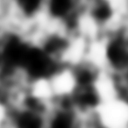
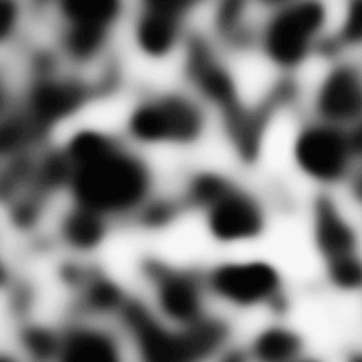
Simulations. – We ran N-body simulations with the CUBEP3M codeMerz et al. (2005), evolving $256^{3}$ particles on a $512^{3}$ grid in a 322$h^{-1}$ Mpc box. The smoothing window $W$ has a width $\sigma=1.25h^{-1}$Mpc. Figure 1 shows a slice of the original and reconstructed smoothed density fields, both once again smoothed on a 8$h^{-1}$ window to reduce the small scale noise. We found little dependence on the windowing scale until we smooth on linear scales, which is related to the information saturation phenomenon discussed below.

Figure 2 shows the raw and reconstructed power spectra, as well as the cross correlation spectrum. The amplitude of the reconstructed spectrum was scaled to match that of the dark matter. In principle, this amplitude is determined for truly Gaussian random fields, but in practice these assumptions do not hold precisely. The amplitude of the cross correlation is now completely determined, and we see a good cross correlation over a decade in wave number.

Figure 2: Simulation results: Dark matter power spectrum (solid line), tidal reconstructed power spectrum (dashed line), cross power spectrum (dotted line). We see good agreement between the reconstructed power spectrum and the dark matter power.

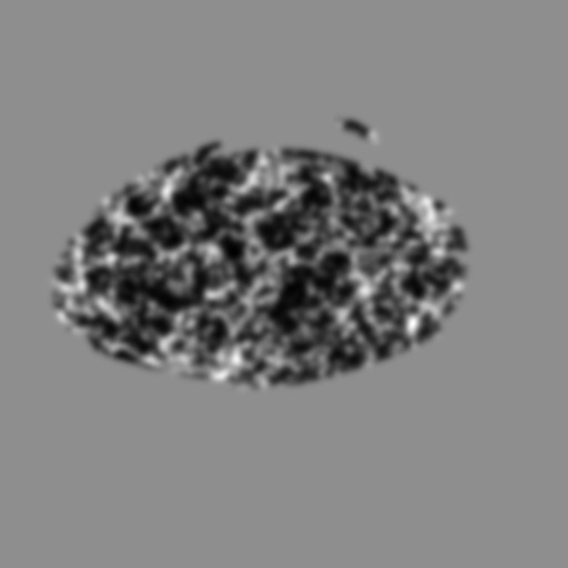
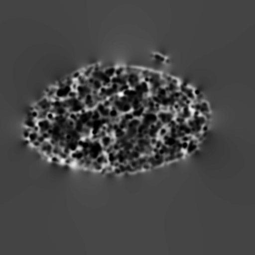
Data. – We also applied the technique to a volume limited subsample of the Sloan Digital Sky Survey (SDSS) in which 112043 galaxies were selected. We constructed a Cartesian mapping as follows: A 0.9$h^{-1}$ Gpc box is centered on the north galactic pole, at $z=0.1$. We used the redshift range $0.7<z<1.3$. The angular position is mapped at 300$h^{-1}$ Mpc per radian, and the radial position at 0.01$h^{-1}$ Mpc/(km/sec). A random catalog with five times as many galaxies was used as a density normalization. The log of the smoothed random density is subtracted from the log of the smoothed galaxy count. Pixels with less than half the peak random galaxy density count were masked. Figure 3 shows a slice of the galaxy and reconstructed density fields at $z=0.1$.

Figure 3: $z=0.1$ slices of SDSS survey embedded in a 900$h^{-1}$ Mpc box, smoothed by a window function. Top panel: Original galaxy field. Bottom panel: dark matter map reconstructed from small scale galaxy density field alignments.

Figure 4: SDSS results: galaxy power spectrum (solid line), tidal reconstructed power spectrum (dashed line), cross power spectrum (dotted line). We see good agreement for the reconstructed power spectrum.

The original and reconstructed power spectra are shown in Figure 4, where we have again scaled the reconstructed power spectrum. When comparing the biased galaxies, the bias will always be a free parameter, such that the non-linear effects of normalization can be absorbed as a relative bias. The cross power spectrum has a cross correlation coefficient $r>0.5$ for all $k$ up to 0.2$h$/Mpc, thereby demomstrating a qualitative successful dark matter reconstruction.

Discussion. – We have seen a successful application of a heuristic tidal field estimator. Here we will discuss the theoretical framework, and future directions.

The large scale tidal shear field is the expectation value of the quadratic outer product

$$T_{ij}\propto\langle(\partial_{i}\bar{\delta})\partial_{j}\bar{\delta}\rangle.$$ (1)

Redshift space distortions complicate every components that include $i=3$. Our shear components are related as $\gamma_{1}=T_{11}-T_{22}$ and $\gamma_{2}=2T_{12}$. It was shown that this two index tensor is proportional to the traceless tidal shear tensor (see eqn(35) ofLu and Pen (2008)) derived from the gravitational potential: $\tilde{T}_{ij}=\partial_{i}\partial_{j}\phi-\frac{\delta_{ij}}{2}\nabla^{2}\phi.$ The trace, which corresponds to the local mean density, in principle transforms in a similar way, however we will defer such study to the future. The trace free estimator is quadratic in the density field, and does not require second order perturbation theory to compute. Being trace free, it does not backreact on the mean density. We are only considering waves in $\phi$ on much larger scales $k_{\phi}$ than the galaxy density $\delta$: $k_{\delta}\gg k_{\phi}$.

The reconstructed density field is derived from a convolution:

$$\kappa=\int T_{ij}(x^{\prime})K_{ij}(x-x^{\prime})d^{3}x^{\prime}$$ (2)

where the kernel $K_{ij}$ is given in Fourier space as

$$K_{ij}(k)=\frac{k^{2}}{k_{x}^{2}+k_{y}^{2}}\left(\hat{k}_{i}\hat{k}_{j}-\frac{\delta_{ij}}{2}\right).$$ (3)

In the limit that the tidal mode is linear and has a wave length much longer then the smoothing scale of the Gaussian window, the perturbative coupling arises solely from the induced gravitational displacement.

Free falling observers are only sensitive to tidal forces, and the tidal force on the window scale is just a stretching of coordinates. The tidal distortion field can be viewed as an integral over the history of gravity. We note that the actual density field only follows linear evolution weakly, even on apparently linear scalesSeljak and Warren (2004).

Relation to CMB Lensing. – The effect described here is identical to the CMB lensing phenomenon, which also induces a three point correlation between two points on the CMB and one in the intervening spaceLewis and Challinor (2006). In our case, two wave vectors are on small scales, and one on large scales, all in the same volume.

Connection to Non-Gaussianity. – Our separation of scales is equivalent to bispectrum calculations in the squeezed limit. We are measuring the variance modulated by a large scale, small $k$ mode, again in analogy with the CMB caseCreminelli et al. (2011). The coordinate change is the leading order effect relevant for the shear, whose measurement corresponds to using only the term dependent on the angle $\alpha$ between the small $k_{\phi}$ vector and the two large ones $k_{\delta}$. Figure 4 is the covariance of $\langle\delta\rangle$, and $\kappa$ is in turn a quadratic function of $\delta$ at large wave numbers. We have effectively integrated the bispectrum over its quadrupole $\int\langle\delta(k_{\phi})|\delta(k_{\delta})|^{2}\rangle\cos(2\alpha)d\alpha$.

This is the leading effect contributing to the information saturation phenomenonMeiksin and White (1999). It was found that the variance in the power spectrum on quasi-linear scales was up to three orders of magnitude larger than expected for Gaussian random fields. This was also observered for variances in the shear estimatorsLu and Pen (2008); Harnois-Deraps and Pen (2011). It had been proposed that this saturation was due to Poisson noise in the virialized halosNeyrinck et al. (2006), however Poisson noise does not lead to an increase in the shear variance, hence can not be the complete picture. The shear has been numerically observed to saturate at a similar information content as the mean variance. Furthermore, reconstruction techniques are able to increase the information contentNgan et al. (2012), which is not expected in a Poisson model.

The cosmic tides picture can qualitatively explain this information saturation effect. A 10% tidal distortion results in a systematic change of the variance by $\sim 10\%$. When more than 100 modes are measured, their variance is dominated by the larger scale shear. An analogous effect applies to the power spectrum variances. This implies that saturation is dominated by modes near the peak of the power spectrum, $k\sim 0.02$.

Recovering Lost 21cm Modes. – 21cm intensity mapping has emerged as a promising technique to map the large scale structure of the universe, at redshifts $z$ from 1 to 10. Unfortunately, many of the key cross correlations with photo-x galaxy and the CMB have been thought to be impossible due to foreground contamination for radial modes with small wave numbersLidz et al. (2009); Adshead and Furlanetto (2008). Our proposed tidal reconstruction technique works best in this regime, and opens up a new set of possibilities.

Reducing Sample Variance. – The high cross correlation seen in the simulation suggests that one can measure the dark matter density on large scales without redshift space distortions. By comparing the galaxy power spectrum to the $\kappa$ power spectrum as a function of angle to the line of sight, one can solve for the velocity contribution. This allows for a measurement of velocity on the same mode as the density, hence determines the velocity growth factor without sample variance, analogous to McDonald and Seljak (2009). In principle, this could enable precision measurements of neutrino masses.

Conclusion. – We have presented a new framework to measure the effects of gravity through its tidal effect on the structure of galaxy clustering. We isolated this effect theoretically from other complications by projecting out mean density changes. The effect becomes analogous to the lensing shear on large scale structure or the CMB. We have tested the dark matter density reconstruction in simulations and with the SDSS data. We found good agreement, with reconstruction noise less than sample variance. This opens up the window for precision measurements of the transfer function, potentially measuring neutrino masses or testing modified gravity.

ULP thanks NSERC, SHAO and NAOC for financial support. XC was supported by grants NSFC 11073024, CAS KJCX3-SYW-N2. N-body computations were performed on the TCS supercomputer at the SciNet HPC Consortium. SciNet is funded by: the Canada Foundation for Innovation under the auspices of Compute Canada; the Government of Ontario; Ontario Research Fund - Research Excellence; and the University of Toronto. We thank Kiyoshi Masui for helpful comments.

References

- Meiksin and White (1999) A. Meiksin and M. White, MNRAS 308, 1179 (1999), eprint arXiv:astro-ph/9812129.
- Lu and Pen (2008) T. Lu and U.-L. Pen, MNRAS 388, 1819 (2008), eprint 0710.1108.
- Masui and Pen (2010) K. W. Masui and U.-L. Pen, Physical Review Letters 105, 161302 (2010), eprint 1006.4181.
- Schneider et al. (1992) P. Schneider, J. Ehlers, and E. E. Falco, Gravitational Lenses (Springer-Verlag Berlin Heidelberg New York. Also Astronomy and Astrophysics Library, 1992).
- Miralda-Escude (1991) J. Miralda-Escude, Astrophys. J. 380, 1 (1991).
- Kamionkowski et al. (1998) M. Kamionkowski, A. Babul, C. M. Cress, and A. Refregier, MNRAS 301, 1064 (1998), eprint arXiv:astro-ph/9712030.
- Pen et al. (2002) U.-L. Pen, L. Van Waerbeke, and Y. Mellier, Astrophys. J. 567, 31 (2002), eprint arXiv:astro-ph/0109182.
- Lu et al. (2010) T. Lu, U.-L. Pen, and O. Doré, Phys. Rev. D 81, 123015 (2010), eprint 0905.0499.
- Harnois-Deraps and Pen (2011) J. Harnois-Deraps and U.-L. Pen, ArXiv e-prints (2011), eprint 1109.5746.
- Weinberg (1992) D. H. Weinberg, MNRAS 254, 315 (1992).
- Merz et al. (2005) H. Merz, U.-L. Pen, and H. Trac, New Astronomy 10, 393 (2005), eprint arXiv:astro-ph/0402443.
- Seljak and Warren (2004) U. Seljak and M. S. Warren, MNRAS 355, 129 (2004), eprint arXiv:astro-ph/0403698.
- Lewis and Challinor (2006) A. Lewis and A. Challinor, Phys. Rep. 429, 1 (2006), eprint arXiv:astro-ph/0601594.
- Creminelli et al. (2011) P. Creminelli, C. Pitrou, and F. Vernizzi, J. Cosmology Astropart. Phys. 11, 25 (2011), eprint 1109.1822.
- Neyrinck et al. (2006) M. C. Neyrinck, I. Szapudi, and C. D. Rimes, MNRAS 370, L66 (2006), eprint arXiv:astro-ph/0604282.
- Ngan et al. (2012) W. Ngan, J. Harnois-Déraps, U.-L. Pen, P. McDonald, and I. MacDonald, MNRAS 419, 2949 (2012), eprint 1106.5548.
- Lidz et al. (2009) A. Lidz, O. Zahn, S. R. Furlanetto, M. McQuinn, L. Hernquist, and M. Zaldarriaga, Astrophys. J. 690, 252 (2009), eprint 0806.1055.
- Adshead and Furlanetto (2008) P. J. Adshead and S. R. Furlanetto, MNRAS 384, 291 (2008), eprint 0706.3220.
- McDonald and Seljak (2009) P. McDonald and U. Seljak, J. Cosmology Astropart. Phys. 10, 7 (2009), eprint 0810.0323.