Einstein-Podolsky-Rosen entanglement and steering in two-well BEC ground states

Abstract

We consider how to generate and detect Einstein-Podolsky-Rosen (EPR) entanglement and the steering paradox between groups of atoms in two separated potential wells in a Bose-Einstein condensate (BEC). We present experimental criteria for this form of entanglement, and propose experimental strategies for detecting entanglement using two or four mode ground states. These approaches use spatial and/or internal modes. We also present higher order criteria that act as signatures to detect the multiparticle entanglement present in this system. We point out the difference between spatial entanglement using separated detectors, and other types of entanglement that do not require spatial separation. The four-mode approach with two spatial and two internal modes results in an entanglement signature with spatially separated detectors, conceptually similar to the original EPR paradox.

I Introduction

The Einstein-Podolsky-Rosen (EPR) paradox EPR paradox established a link between entanglement and nonlocality Bell in quantum mechanics. The extent to which entanglement can exist in spatially separated macroscopic and massive systems is still essentially unknown. Entanglement in optics however has been extensively studied and numerous experiments have shown evidence for it entoptics ; aspect ; kwiatzeil ; ou ; eprcrit ; rmp . An important distinction is that optical entanglement involves (nearly) massless particles, and hence is a much less rigorous test of any gravitational effects present.

Generation of EPR entanglement between two massive systems therefore represents an important challenge. Such entanglement is a step in the direction of fundamental tests of quantum mechanics, and is relevant to the long term quest for understanding the relationship between quantum theory and gravity. Ultimately, one would like to demonstrate spatially entangled mass distributions, and this appears much more promising for ultra-cold atoms than for room-temperature atoms. For this reason, we focus on ultra-cold BEC environments here. This is also relevant if BEC interferometry is to be useful to those areas of quantum information and metrology where entanglement is known to give an advantage Leeprl ; eprappli ; spinsqwine ; holburn ; dowlent ; fisher ; naturepryentph . In this paper, we study strategies for generation of EPR entanglement between Bose-Einstein condensates (BEC) confined to two spatially separated potential wells.

Quantum correlations and EPR tests for Bose-Einstein condensates have been suggested previously, with strategies involving molecular down-conversion Moleccorrel and four wave mixing interactions GardinerDeuar ; olsenferris ; coldmolebell , among others. Early experiments measuring free-space correlations demonstrated promising signatures of increased fluctuations associated with entanglement Kasevich ; Jin , but were unable to conclusively demonstrate entanglement or squeezing via reduced fluctuations, largely due to measurement inefficiencies. This has improved with recent multi-channel plate detection methods, but detection efficiency still remains an issue westbrook . Entanglement has also been measured, very recently, for distinct but nearly spatially superimposed modes neweprbec ; eprenthiedel ; science pairs ent in an optical lattice.

Here, we are motivated to study the two well case, in view of experiments that have used this or similar systems to confirm both sub-shot noise quantum correlations esteve , and multiparticle entanglement among a small group of atoms Gross2010 ; Philipp2010 . For much larger numbers of atoms ($\sim 40,000$), nearly quantum limited interferometry has been recently verified Egorov , showing that trapped atom interferometry has the potential to reach mesoscopic sizes. There have also been a number of previous theoretical studies bargill ; bectheoryepr that outline different proposals and entanglement signatures.

The goal of this paper is to first clarify what it means to have an EPR entanglement between groups of atoms in a BEC, and to outline a strategy for achieving this goal. We define EPR entanglement as being that entanglement existing between two spatially separated systems, so that an EPR paradox can be realised. For EPR entanglement to be claimed, three properties are to be evident rmp :

1. Two systems must be shown entangled through local measurements at spatially distinct locations.

2. The nature of the entanglement criterion should confirm an EPR paradox. This requires measurement of sufficiently strong correlation between the two systems, for two non-commuting “EPR” observables such as position/ momentum, conjugate spins, or quadrature phase amplitudes eprcrit . A generalised approach would allow other entanglement measures, such as those for “EPR steering” Schrodinger ; hw-steering-1 ; hw2-steering-1 ; EPRsteering-1 ; hw-np-steering-1 ; asymmurray ; multiqubits-1 ; loopholefreesteering which reveal an inconsistency between EPR’s local realism and the completeness of quantum mechanics using more general measurement strategies.

3. To fully justify EPR’s no “spooky action-at-a-distance” assumption EPR paradox , the measurement events should be causally separated Bell ; aspect ; kwiatzeil .

For large groups of atoms, the task of detecting EPR entanglement is much more feasible when the emphasis is on the EPR paradox itself, rather than on the failure of Bell’s local hidden variable model Bell . This leaves room for the possibility of confirming multiparticle entanglement, a subject we touch on briefly in this paper. For spatially separated systems, the detection of sufficient correlation of locally defined EPR observables so that entanglement is confirmed Duan-simon-1 ; simon-1 ; proof for product form would represent an achievable first benchmark. This by itself is not direct evidence for the EPR paradox, or quantum steering, although it is a necessary condition. The second step of confirming the paradox has been carried out for photons rmp , and also appears achievable for atoms. The last step is probably the most difficult for atoms. It would require either very fast measurements in one vacuum chamber, or hybrid techniques involving two separated BECs with coupling via atom-photon interfaces Interface , in order to achieve causally separated measurement.

There are many possible strategies for generation of spatial EPR entanglement. Early experiments employed two photon cascades and, later, optical parametric down conversion, to generate entangled photon pairs entoptics ; aspect ; kwiatzeil . Continuous variable EPR entanglement between two fields, in a so-called “two-mode squeezed state” caves sch , was also generated using parametric down conversion ou ; eprcrit ; eprparamp . Such entanglement gave evidence for an EPR paradox rmp , although true causal separation of measurement events was not demonstrated in these experiments.

The paper is arranged as follows. In Section II we give a general introduction to the different possible entanglement strategies. Section III focuses on signatures for demonstrating entanglement, pointing out the hierarchy of nonlocality measures including EPR-steering hw-steering-1 and Bell’s nonlocality Bell , as well as signatures for detecting multiparticle entanglement. Section IV considers entanglement preparation in a two-well system, modeled as two modes with boson operators $a$ and $b$ Leeprl . In this case, the S-wave scattering intra-well interactions, given by Hamiltonians $H=ga^{\dagger 2}a^{2}$ and $H=gb^{\dagger 2}b^{2}$, provides a local nonlinearity at each well, while the coupling or tunneling inter-well term, modeled as $H=\kappa(a^{\dagger}b+ab^{\dagger})$ generates inter-well entanglement. Here the intra- and inter-well interactions act simultaneously, to enhance entanglement formation in the ground state. Section V treats a four-mode generalization of this, which has the advantage that EPR-entanglement can be measured using atom counting at each site, without the use of a local oscillator. Our conclusions are summarized in Section VI, with details given in the Appendices. This paper is based on preliminary work presented in a Letter bectheoryepr . A second class of entanglement strategies using dynamical techniques will be analyzed in a subsequent paper.

II Entanglement Strategies

II.1 Prototype states for two-mode entanglement

Suppose two spatially separated systems are describable as distinct modes, represented by boson operators $a$ and $b$. There are two prototype states that one can consider, that can give multiparticle EPR entanglement. The first, which we call particle-pair generation, is currently the most widely known and used ou . We consider an entangled state with number correlations:

$$|\psi\rangle_{II}=\sum_{n=0}^{\infty}c_{n}|n\rangle_{a}|n\rangle_{b}.$$ (1)

This type of two-mode squeezed state gives two-particle correlations arising from a pair production process $H=\kappa a^{\dagger}b^{\dagger}+\kappa^{*}ab$ where $\langle ab^{\dagger}\rangle=0$ but $\langle ab\rangle\neq 0$, and the number difference is always squeezed number french ; lane abs . These EPR states are formed in optics with parametric down conversion eprcrit ; rmp , and similarly in nondegenerate four wave mixing four wave mixing squeezing . Since they are not number-conserving, they are not typical of states formed in coupled two-well experiments, although they have been generated in recent BEC experiments using spin or mode-changing collisions neweprbec ; eprenthiedel ; science pairs ent .

In this paper, we will focus on a second form of EPR entanglement, which we call number conserving. This occurs, for example, when fixed number states are input into a beam splitter: $H=\kappa(a^{\dagger}b+ab^{\dagger})$, so that $\langle ab\rangle=0$ but $\langle ab^{\dagger}\rangle\neq 0$. We consider an entangled number-conserving state of form bec well ham cirac ; gerdan ; gorsav ; wellbecmurr ; supbec ; carr :

$$|\psi\rangle_{I}=\sum_{n=0}^{N}c_{n}|n\rangle_{a}|N-n\rangle_{b}.$$ (2)

This is the closest to the state prepared in some recent two-well BEC experiments, where the total number is conserved esteve ; Gross2010 . We will examine how to unambiguously detect two-mode entanglement, and EPR steering entanglement, for these states.

II.2 Experimental strategies

Before examining detailed solutions for an interacting BEC, it is useful to summarize how two-mode number-conserving entanglement can be generated, in schematic form. We consider how to generate entanglement between two groups of atoms in separated potential wells in a BEC. What is useful is a combination of nonlinear local interactions to generate a nonclassical squeezed state in each well - together with a nonlocal linear interaction to produce the entanglement between two spatially distinct locations. In the case of the BEC, the S-wave scattering can provide a nonlinear local interaction, and quantum diffusion across a potential barrier acts like a beam-splitter to provide the final nonlocal linear interaction. Both effects occur at the same time in the schemes treated here, in Sections IV and V.

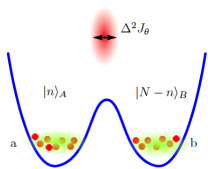
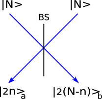
We show in Section IV that the entanglement generated for the two-well ground state with a fixed number of atoms can translate to an EPR steering type of entanglement hw-steering-1 ; multiqubits-1 (Fig. 1). For an actual demonstration of this sort of EPR entanglement, however, one must use signatures that involve local measurements, for two spatially separated observers (often called Alice and Bob), at sites $A$ and $B$. One can use local oscillator (LO) measurements at each site, that provide phase shifts or their equivalent between the measured and LO modes olsenferris ; eprenthiedel . In Section V, we propose an alternative though similar four-mode strategy, as shown in Fig. 2. We summarise the two types of gedanken-experiment as follows:

Figure 1: (Color online) Two mode case: A double-well, one spin orientation BEC. $a,$$b$ are operators for two modes at $A$ and $B$. The $a$ and $b$ are prepared with a two mode number difference squeezing and an entanglement, by adiabatic cooling to the ground state. We develop signatures to detect the inter-well entanglement, using inter-well spin operators.

• Two-mode entanglement preparation then analysis: the entangled state is generated as the two-mode ground state in a double-well potential (Fig. 1). Experimentally, this appears relatively simple, involving evaporative cooling to the ground state in a single well followed by an adiabatic ramping of an optical lattice to provide the central potential barrier Bloch ; esteve . However, there are two levels of experimental demonstration of the entanglement. The simplest involves a nonlocal measurement that recombines the two modes, to demonstrate an interwell entanglement. For demonstration of the EPR steering paradox, however, strictly local measurements must be used. EPR steering entanglement can be detected with a phase sensitive “local oscillator” measurement at each well, though this may represent an experimental challenge. This strategy is discussed in Section IV.

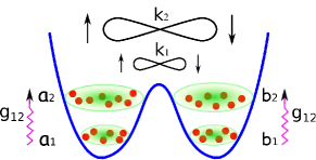
• Four-mode entanglement preparation then analysis: we consider four-mode states created through cooling in a double-well potential with two spin states in each well (Fig. 2). Experimentally, this is more complex, but an EPR steering entanglement can be demonstrated using local Rabi rotations of the two spins of each well. This strategy is discussed in Section V.

Figure 2: (Color online) Four-mode case: A double-well, two spin orientation BEC. We suppose the modes $a_{i}$ and $b_{i}$ are spatially separated. Modes $a_{1}$, $a_{2}$ could be different spatial modes, or different spin components of the same well. Pairs $a_{1}$, $b_{1}$ (and $a_{2}$, $b_{2}$) can become entangled, due to the inter-well couplings. We allow for the asymmetric case where pair $a_{2}$ and $b_{2}$ have much greater numbers than $a_{1}$ and $b_{1}$ ($N_{2}\gg N_{1}$) and also consider a case where modes $a_{2}$ and $b_{2}$ need not be entangled ($\kappa_{2}=0$).

In both two and four mode cases, the basic idea is:

1. Correlated ground state preparation, through evaporative cooling in a potential well with linear coupling between wells.

2. Local Rabi rotation (in the four-mode case) to a superposition of internal spins, thus choosing an EPR measurement angle. In the two mode case, entanglement can be detected by nonlocal rotation of the two spins.

3. Measurement, usually from absorption imaging, giving occupation numbers.

III Entanglement and EPR Steering criteria

In the original EPR proposal EPR paradox , the paradox arose from correlations between the positions and momenta of two particles emitted from the same source. With optical or atomic Bose fields, one can define the quadrature phase amplitudes of the modes, as $X_{A}=a^{\dagger}+a,$ and $Y_{A}=(a^{\dagger}-a)/i$, and similarly for mode $b$. These have similar commutators to position and momentum in the particle system. Detection of sufficient correlation between the quadratures will signify entanglement Duan-simon-1 ; simon-1 , and the EPR paradox eprcrit , as analysed recently for atoms by Gross et al eprenthiedel .

We find that the common approach of detecting the EPR correlation as a reduced variance Duan-simon-1 ; eprcrit is not so useful for the number conserving entangled states (2). Instead, we adapt the criteria proposed by Hillery and Zubairy hillzub , and Cavalcanti et al CFRD ; multiqubits-1 ; zubhighmomentbell ; bellcfrdnew ; bellcfrdpra . Like most practical criteria to date, these methods are sufficient, but not necessary, for the detection of entanglement. The limitations of measures of entanglement based on purity have been pointed out recently by Chianca and Olsen ch olsen ent measurewell .

III.1 Two-mode Hillery-Zubairy entanglement criterion

Two subsystems $A$ and $B$ are said to be entangled if the density operator $\rho$ for the composite system cannot be expressed as a mixture of product states ie.

$$\rho=\sum_{R}P_{R}\rho_{A}^{R}\rho_{B}^{R}$$ (3)

fails, where $\sum_{R}P_{R}=1$, and $\rho_{A/B}^{R}$ is a density operator for $A/B$.

Consider where systems are single field modes with boson operators $a$ and $b$ respectively. Hillery and Zubairy (HZ) showed that the two modes $a$ and $b$ are entangled if hillzub

$$|\langle a^{m}\left(b^{\dagger}\right)^{n}\rangle|^{2}>\langle\left(a^{\dagger}\right)^{m}a^{m}\left(b^{\dagger}\right)^{n}b^{n}\rangle.$$ (4)

All separable states (defined as those for which (3) holds) satsify $|\langle a^{m}\left(b^{\dagger}\right)^{n}\rangle|^{2}\leq\langle\left(a^{\dagger}\right)^{m}a^{m}\left(b^{\dagger}\right)^{n}b^{n}\rangle$.

In Ref bectheoryepr , we suggested how to rewrite criterion (4) for $m=n$. For any nonhermitian operator $Z$, we consider the generalized variance, which must be nonnegative:

$$\Delta^{2}Z\equiv\langle\left(Z^{\dagger}-\langle Z^{\dagger}\rangle\right)\left(Z-\langle Z\rangle\right)\rangle=\langle Z^{\dagger}Z\rangle-\langle Z^{\dagger}\rangle\langle Z\rangle\geq 0\,.$$ (5)

Defining $Z=a^{m}\left(b^{\dagger}\right)^{m}$, we find it is always true (for any state) that

$$|\langle a^{m}b^{\dagger m}\rangle|^{2}-\langle a^{\dagger m}a^{m}b^{\dagger m}b^{m}\rangle \leq \langle a^{\dagger m}a^{m}([b^{m}b^{\dagger m},b^{\dagger m}b^{m}])\rangle.$$

Thus, the HZ criterion (4) confirms entanglement if:

$$0\leq E_{HZ}^{(m)} = 1+\frac{\langle a^{\dagger m}a^{m}b^{\dagger m}b^{m}\rangle-|\langle a^{m}b^{\dagger m}\rangle|^{2}}{\langle a^{\dagger m}a^{m}(b^{m}b^{\dagger m}-b^{\dagger m}b^{m})\rangle}<1.$$

It is also possible to derive a criterion using the commutators for mode $a$. Hence the HZ entanglement criterion (LABEL:eq:HZentcritm) is best written with the optimal choice of denominator, corresponding to the minimum of $\langle a^{\dagger m}a^{m}(b^{m}b^{\dagger m}-b^{\dagger m}b^{m})\}$ or $\langle b^{\dagger m}b^{m}(a^{m}a^{\dagger m}-a^{\dagger m}a^{m})\rangle$.

The first order ($m=n=1$) HZ criterion for entanglement becomes

$$0<E_{HZ}^{(1)} = 1+\frac{\langle a^{\dagger}ab^{\dagger}b\rangle-|\langle ab^{\dagger}\rangle|^{2}}{min\{\langle a^{\dagger}a\rangle,\langle b^{\dagger}b\rangle\}}<1.$$ (8)

III.2 Multiparticle entanglement criterion

The second order HZ entanglement criterion is obtained by using the power $m=2$ with the identity $[b^{2}b^{\dagger 2},b^{\dagger 2}b^{2}]=4b^{\dagger}b+2$. Entanglement is then observed if

$$0\leq E_{HZ}^{(2)} = 1+\frac{\langle a^{\dagger 2}a^{2}b^{\dagger 2}b^{2}\rangle-|\langle a^{2}b^{\dagger 2}\rangle|^{2}}{\langle a^{\dagger 2}a^{2}(4b^{\dagger}b+2)\rangle}<1.$$

We now show that the higher order HZ entanglement criterion (LABEL:eq:HZentcritm) with $m>1$ enables detection of multi-particle entanglement. The criterion (LABEL:eq:hzsecond-1) can only be satsified if there exists a nonzero probability that the system is in an entangled superposition state of the form

$$|\psi\rangle=c|n_{A}\rangle|n_{B}\rangle+d|n_{A}+m\rangle|n_{B}^{\prime}\rangle+\sum_{n,l}c_{nl}|n\rangle|l\rangle$$ (10)

(or that obtained by interchanging the states of $A$ and $B$) where the amplitudes $c,d\neq 0$ but $c_{nl}$ are unspecified. Here $|n_{A}\rangle|n_{B}\rangle$ is the product number state with $n_{A}$ particles in $A$ and $n_{B}$ particles in $B$.

Proof: Any composite system $A$/ $B$ can be described by a density matrix $\rho=\sum_{R}P_{R}\rho_{sep}^{R}+\sum_{R^{\prime}}P_{R^{\prime}}\rho_{ent}^{R^{\prime}}$, where $\rho_{sep}^{R}$ and $\rho_{ent}^{R^{\prime}}$ represent pure separable and entangled states respectively. The higher-order HZ entanglement measure (4) with $m=n$ can therefore be written as a ratio

$$R=\frac{|\langle a^{m}\left(b^{\dagger}\right)^{m}\rangle|^{2}}{\langle\left(a^{\dagger}\right)^{m}a^{m}\left(b^{\dagger}\right)^{m}b^{m}\rangle}$$ (11)

where

$$\langle a^{m}\left(b^{\dagger}\right)^{m}\rangle = \sum_{R}P_{R}\langle a^{m}\left(b^{\dagger}\right)^{m}\rangle_{R}+\sum_{R^{\prime}}P_{R^{\prime}}\langle a^{m}\left(b^{\dagger}\right)^{m}\rangle_{R^{\prime}}$$

and

$$\langle\left(a^{\dagger}\right)^{m}a^{m}\left(b^{\dagger}\right)^{m}b^{m}\rangle = \sum_{R}P_{R}\langle\left(a^{\dagger}\right)^{m}a^{m}\left(b^{\dagger}\right)^{m}b^{m}\rangle_{R}$$

$$+\sum_{R^{\prime}}P_{R^{\prime}}\langle\left(a^{\dagger}\right)^{m}a^{m}\left(b^{\dagger}\right)^{m}b^{m}\rangle_{R^{\prime}}$$

Here $\langle O\rangle_{R}$ represents the expectation value of $O$ for state $\rho_{R}$. Since for a separable state, $R\leq 1$, we can see that if $\sum_{R^{\prime}}P_{R^{\prime}}\langle a^{m}\left(b^{\dagger}\right)^{m}\rangle_{R^{\prime}}=0$, it is always the case that $\rho$ predicts $R\leq 1$. In short, the higher order entanglement, $E_{HZ}^{(m)}<1$, cannot be achieved unless there is a nonzero probability $P_{R^{\prime}}$ for a pure entangled state $\rho_{ent}^{R^{\prime}}$ for which $\langle a^{m}\left(b^{\dagger}\right)^{m}\rangle\neq 0$. Expanding $\rho_{ent}^{R^{\prime}}$ in terms of the number state basis $|n_{A}\rangle|n_{B}\rangle$ where yields $\rho_{ent}^{R^{\prime}}=|\psi\rangle\langle\psi|$, where

$$|\psi\rangle=\sum_{n,l}c_{nl}|n\rangle_{A}|l\rangle_{B}.$$ (12)

If only adjacent number states $|n\rangle$, $|n+1\rangle$ have nonzero amplitude $c_{nl}$, the $\langle a^{m}(b^{\dagger})^{m}\rangle=0$ where $m>1$. Hence, the superposition (12) necessarily includes number states separated by $m$.

III.3 Two-mode EPR-steering criterion

Nonlocality can be revealed using criteria similar to (4). Entanglement itself does not imply an EPR-steering paradox EPR paradox ; eprcrit ; hw-steering-1 ; EPRsteering-1 nor violation of local hidden variable theories (Bell’s theorem) CFRD ; zubhighmomentbell ; bellcfrdnew ; bellcfrdpra ; HDRspin ; multiqubits-1 , which are seen as stronger forms of entanglement. In this paper, we consider two sites only, and focus on the entanglement and EPR-steering cases, since it has been shown that violation of the moment Bell inequality derived in Ref CFRD requires three or more sites bellcfrdnew .

The EPR paradox was discussed by Schrodinger Schrodinger , who introduced the notion of “steering” as an apparent action-at-a-distance. Criteria for “steering” can be developed using the asymmetric local hidden state separable model of Wiseman and co-workers hw-steering-1 . Violation of this model reveals inconsistency of EPR’s asymmetric local realism with the completeness of quantum mechanics, and thus may be thought of as a generalized EPR paradox hw-steering-1 ; hw2-steering-1 ; EPRsteering-1 ; rmp . The EPR paradox-steering nonlocality has been realised experimentally in loop-hole free and high efficiency scenarios for optical qubits loopholefreesteering and Gaussian states ou ; rmp .

An EPR-steering nonlocality is detected if

$$|\langle a^{m}b^{\dagger n}\rangle|^{2} > \langle a^{\dagger m}a^{m}(\frac{b^{\dagger n}b^{n}+b^{n}b^{\dagger n}}{2})\rangle.$$ (13)

The proof follows from straightforward application of methods is given in multiqubits-1 which derived this EPR steering criterion for $m=n=1$. This criterion can also be rewritten in terms of the HZ entanglement parameter (8), so that EPR-steering entanglement is confirmed if:

$$0\leq E_{HZ}^{(m)} = 1+\frac{\langle a^{\dagger m}a^{m}b^{\dagger m}b^{m}\rangle-|\langle a^{m}b^{\dagger m}\rangle|^{2}}{\langle a^{\dagger m}a^{m}(b^{m}b^{\dagger m}-b^{\dagger m}b^{m})\rangle}<\frac{1}{2}.$$

We note that the moments of type $\langle a^{m}b^{\dagger n}\rangle$ are in principle measured as a linear combination of moments of the Hermitian observables, $X_{A}$ and $P_{A}$, and $X_{B}$ and $P_{B}$.

III.4 Two-mode spin entanglement and EPR steering criteria

It is convenient to quantify entanglement using spin-operator methods, the advantage being that for BEC two-well systems, the variances of Schwinger spins have been measured in experiment esteve . Hillery and Zubairy hillzub have written the first order criterion (4) in terms of the variances of inter-well Schwinger spins, defined as:

$$J_{AB}^{X} = \left(a^{\dagger}b+ab^{\dagger}\right)/2$$

$$J_{AB}^{Y} = \left(a^{\dagger}b-ab^{\dagger}\right)/(2i)$$

$$J_{AB}^{Z} = \left(a^{\dagger}a-b^{\dagger}b\right)/2$$

$$J_{AB}^{2} = \hat{N}_{AB}(\hat{N}_{AB}+2)/4$$

$$\hat{N}_{AB} = a^{\dagger}a+b^{\dagger}b\,.$$ (15)

Where the outcomes for $\hat{N}_{AB}$ are fixed at $N$, the spin is fixed as $J=N/2$. The HZ entanglement criterion given by Eq. (8) for $m=n=1$ can then be rewritten as:

$$0<E_{HZ} = \frac{\left(\Delta J_{AB}^{X}\right)^{2}+\left(\Delta J_{AB}^{Y}\right)^{2}}{\langle\hat{N}_{AB}\rangle/2}<1.$$ (16)

We recall from (LABEL:eq:eprsteerhz) that EPR steering is observed if

$$0<E_{HZ} <1/2.$$ (17)

It should be noted here that this type of spin-operator variance has been measured experimentally esteve by observing the interference between the two modes, on expanding the atomic clouds after turning the traps off. However, as we discuss later, this strategy cannot be readily interpreted in the EPR sense, due to the lack of separation during measurement.

The best entanglement (for a fixed number of atoms $N$) as measured by (16) is given when the sum of the two variances of $J_{AB}^{X}$ and $J_{AB}^{Y}$ is minimized. This sum can never be zero, meaning that the ideal entanglement of $E_{HZ}=0$ cannot be reached, because the spins $J_{AB}^{X}$ and $J_{AB}^{Y}$ do not commute. However, the sum becomes asymptotically small for large $N$, in which case large noise appears in the third spin $J_{AB}^{Z}$. The lower bound for the sum of the two variances has been obtained by cj :

$$\frac{\left(\Delta J_{AB}^{X}\right)^{2}+\left(\Delta J_{AB}^{Y}\right)^{2}}{J}\geq C_{J}/J$$ (18)

where the coefficients $C_{J}$ are given in that reference. The reduction of the sum $\left(\Delta J_{AB}^{X}\right)^{2}+\left(\Delta J_{AB}^{Y}\right)^{2}$ below the standard quantum limit (given by $J=\langle\hat{N}_{AB}\rangle/2$) is referred to as “planar squeezing”, and represents the onset of HZ entanglement.

Inequalities of the type (18) are useful for inferring multiparticle entanglement. The level of entanglement as measured by $E_{HZ}$ can give information about how many atoms are involved in the entangled state. Since a large spin $J$ can only be obtained where the number of atoms $N$ is large, very small squeezing necessarily implies an entangled state with a large mean $\langle N\rangle$. This approach was developed by Sorenson and Molmer sorsolm , who explained how to infer a multiparticle entanglement from the level of reduction in the “spin squeezing” variance of $J_{Z}$ Gross2010 ; Philipp2010 .

III.5 Four-mode spin EPR entanglement criteria

A true EPR experiment would involve coherent combination of second fields or condensates at each site, as depicted schematically in Fig. 2. To observe true EPR entanglement between sites $A,B$, a useful procedure is to use two modes per EPR site. Local intra-well spin measurements are defined: for well $A$,

$$J_{A}^{X} = \left(a_{1}^{\dagger}a_{2}+a_{2}^{\dagger}a_{1}\right)/2,$$

$$J_{A}^{Y} = \left(a_{1}^{\dagger}a_{2}-a_{2}^{\dagger}a_{1}\right)/(2i),$$

$$J_{A}^{Z} = \left(a_{2}^{\dagger}a_{2}-a_{1}^{\dagger}a_{1}\right)/2,$$

$$\hat{N}_{A} = a_{2}^{\dagger}a_{2}+a_{1}^{\dagger}a_{1}.$$ (19)

Here $a_{1,2}$ are mode operators for different components of the same site, typically different spatial modes or different nuclear spins at each site. We will also introduce the notation for the corresponding raising and lowering spin operators, $J_{A}^{\pm}=J_{A}^{X}+iJ_{A}^{Y}$. Similar spin operators are defined for site $B$. This defines complementary observables that are locally measurable at each site, using Rabi rotations and number-difference measurements. Calculations of spin correlations at two sites can be carried out most simply on imaging on a micron scale, then dividing the imaged atoms into two halves for measurement purposes. A more sophisticated method is to add a time-dependent external potential to divide the condensate into two widely separated parts. While this gives results that depend on the potential, it provides a physical separation between the sites.

Having defined local spin operators, we now need to consider a suitable EPR entanglement measure. Previous authors have derived HZ-type entanglement and EPR steering criteria that are expressed in terms of these effective local spin operators hillspinpapers ; spinhillery ; mulithillery ; HDRspin . Entanglement is confirmed if

$$\mid\langle J_{A}^{+}J_{B}^{-}\rangle\mid^{2} > \langle J_{A}^{+}J_{A}^{-}J_{B}^{+}J_{B}^{-}\rangle.$$ (20)

This inequality uses operators which are measurable locally using Rabi rotations and number measurements Gross2010 . Criteria involving higher moments are also possible, but are not examined here. As for the original HZ criterion, the spin criterion can be rewritten using the procedure outlined in bectheoryepr . If we define $Z=J_{A}^{+}J_{B}^{-}$, then we can easily show that $\Delta^{2}\left(J_{A}^{+}J_{B}^{-}\right)=\langle J_{A}^{+}J_{A}^{-}J_{B}^{+}J_{B}^{-}\rangle-\langle[J_{A}^{+},J_{A}^{-}]J_{B}^{+}J_{B}^{-}\rangle-|\langle J_{A}^{+}J_{B}^{-}\rangle|^{2}\geq 0.$ Thus,

$${\color[rgb]{0,0,0}|\langle J_{A}^{+}J_{B}^{-}\rangle|^{2}-\langle J_{A}^{+}J_{A}^{-}J_{B}^{+}J_{B}^{-}\rangle} {\color[rgb]{0,0,0}\leq} {\color[rgb]{0,0,0}\langle[J_{A}^{-},J_{A}^{+}]J_{B}^{+}J_{B}^{-}\rangle}$$ (21)

$${\color[rgb]{0,0,0}=} {\color[rgb]{0,0,0}2\langle J_{A}^{Z}J_{B}^{+}J_{B}^{-}\rangle.}$$

Similarly, defining $Z^{\dagger}=J_{A}^{-}J_{B}^{+}$, one can show that

$$|\langle J_{A}^{+}J_{B}^{-}\rangle|^{2}-\langle J_{A}^{+}J_{A}^{-}J_{B}^{+}J_{B}^{-}\rangle \leq 2\langle J_{A}^{+}J_{A}^{-}J_{B}^{Z}\rangle.$$ (22)

The spin entanglement criterion (20) becomes

$$E_{HZ}^{spin\,(1)} \frac{\Delta^{2}\left(J_{A}^{+}J_{B}^{-}\right)}{min[2\langle J_{A}^{Z}J_{B}^{+}J_{B}^{-}\rangle,2\langle J_{A}^{+}J_{A}^{-}J_{B}^{Z}\rangle]}<1\,$$ = (23)

i.e. HZ-type spin entanglement is verified if $E_{HZ}^{spin\,(1)}<1$.

We have derived the spin EPR steering inequalities based on (20) in a previous paper HDRspin . EPR steering is detected if

$$|\langle J_{A}^{+}J_{B}^{-}\rangle|^{2} > \langle[(J_{A})^{2}-(J_{A}^{Z})^{2}\pm J_{A}^{Z}]$$ (24)

$$\ \ \times[(J_{B})^{2}-(J_{B}^{Z})^{2}]\rangle,$$

which can be rewritten as

$$0\leq E_{HZ}^{spin\,(1)} = 1+\frac{\langle J_{A}^{+}J_{A}^{-}J_{B}^{+}J_{B}^{-}\rangle-|\langle J_{A}^{+}J_{B}^{-}\rangle|^{2}}{min[2\langle J_{A}^{Z}J_{B}^{+}J_{B}^{-}\rangle,2\langle J_{A}^{+}J_{A}^{-}J_{B}^{Z}\rangle]}<\frac{1}{2}.$$

We note the spin moments of Eqs (23) and (LABEL:eq:spinhzeprcritvar) are actually measured via the $x$ and $y$ spin components, for example, using the expansion:

$$\langle J_{A}^{+}J_{B}^{-}\rangle= \langle J_{A}^{X}J_{B}^{X}- iJ_{A}^{X}J_{B}^{Y}+J_{A}^{Y}J_{B}^{X}+J_{A}^{Y}J_{B}^{Y}\rangle.$$

IV generation of two-mode entanglement

We next turn to physical means to generate and measure entanglement and EPR-steering in two-mode physical systems. We focus here on the gedanken-experiment of Fig 1, with explicit spatial separation of the two modes.

IV.1 Linear beam splitter with fixed number input states

Possibly the simplest number-conserving entangled state is obtained with a number-squeezed input, together with a beam splitter interaction

$$H=\kappa a^{\dagger}b+\kappa^{*}ab^{\dagger}\,,$$ (27)

which models the exchange of atoms that can take place between wells.

Figure 3: (Color online) A Fock number state $|N\rangle$ incident on a beam splitter produces an entangled state (2).

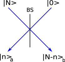
On defining output ($a$, $b$), input ($a_{in}$) and vacuum ($a_{v}$) input modes (Fig. 3, 5), one can write the beam splitter transformation as

$$a = (a_{in}+a_{v})/\sqrt{2}$$ (28)

$$b = (a_{in}-a_{v})/\sqrt{2}.$$

IV.1.1 Single number-state input

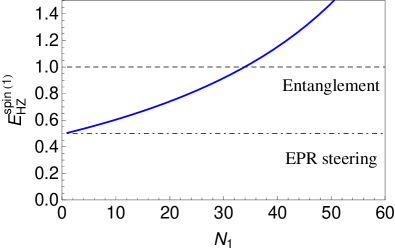
We first consider the simplest case of $N$ atoms input to one port of the beam splitter (Fig. 3). This is equivalent to the linear interferometer case Gross2010 in which a fixed number of atoms are initially in one BEC well. These are then redistributed between wells via a number conserving mechanism. Using (28), the final state is number-conserving (2):

$$|out\rangle = \sum_{n=0}^{N}c_{n}|n\rangle_{a}|N-n\rangle_{b}\,,$$ (29)

where $c_{n}=\sqrt{N!}/\sqrt{2^{N}n!(N-n)!}$. This state (29) is entangled for all $N$. The entanglement can be detected using the Hillery and Zubairy entanglement measure (LABEL:eq:HZentcritm). The superposition (29) clearly involves up to $N$ particles. This multiparticle entanglement can be detected using the higher order entanglement $E_{HZ}^{(n)}$ criteria (LABEL:eq:HZentcritm). Higher order (up to $N$-th) entanglement becomes evident in (Fig. 4).

Figure 4: (Color online) A single Fock number state with beamsplitter is entangled ($E_{HZ}<1$) by the HZ entanglement criteria, Eq. (LABEL:eq:HZentcritm). Higher order entanglement is indicated by the dashed lines. The correlation does not confirm EPR-steering entanglement from Eq. (LABEL:eq:eprsteerhz), which requires $E_{HZ}<0.5$.

This linear beam splitter method generates a relatively small degree of entanglement, however, (Fig. 4), and will later be compared with the much more significant entanglement obtainable using nonlinear BEC interactions.

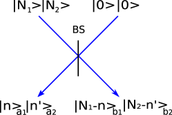
IV.1.2 Double number state input

We next consider a double Fock number state $|N\rangle|N\rangle$ incident on a beam splitter (Fig. 5), as a model for the case where there is initially a fixed, equal number of atoms in each well.

Figure 5: (Color online) A double Fock number state incident on a beam splitter also produces a number-conserving entangled state.

The output state after an exchange between the wells is

$$|out\rangle = \sum_{n=0}^{N}c_{n}|2n\rangle_{a}|2(N-n)\rangle_{b}$$ (30)

where $c_{n}=(-1)^{N-n}\sqrt{(2n)!}\sqrt{\left(2(N-n)\right)!}/\left[2^{N}n!(N-n)!\right]$. In this case, entanglement is again present for all $N$, but cannot be detected via the first order entanglement criterion (8).

Figure 6: (Color online) HZ entanglement criterion using a double Fock number state and beam splitter. The graph shows the criterion (LABEL:eq:HZentcritm) for $m=n=2$ (solid blue line), and $m=n=4$ (red dashed line). EPR-steering is observable with $m=n=2$ and $N<5$.

Entanglement can however be detected via the second order HZ entanglement criterion Eq. (LABEL:eq:hzsecond-1), which indicates an entanglement involving a superposition of number states different by two particles (proved in Section III.B). The fourth-order entanglement $E^{(4)}$ is also evident, indicating superpositions involving states separated by four particles. The entanglement measure $E^{(2)}$ is sufficiently strong that EPR steering can also be confirmed via Eq. (LABEL:eq:eprsteerhz) with $m=n=2$, as shown in Fig. 6, though this effect is diminished for higher $N$.

IV.2 Nonlinear case: BEC ground state

We now examine how to enhance the entanglement over the linear case above, by using a local number-conserving nonlinearity.

We solve for the ground state of a two-component BEC (Fig. 1), as modeled by the following two-mode Hamiltonian gerdan ; Leeprl ; wellbecmurr ; esteve :

$$H=\kappa(a^{\dagger}b+ab^{\dagger})+\frac{g}{2}[a^{\dagger}a^{\dagger}aa+b^{\dagger}b^{\dagger}bb].$$ (31)

Here $\kappa$ denotes the conversion rate between the two components, denoted by the mode operators $a$ and $b$, and $g\propto a_{3D}$ is the nonlinear self interaction coefficient gerdan , proportional to the three-dimensional S-wave scattering length, $a_{3D}$. The first term proportional to $\kappa$ describes an exchange of particles between the two wells (modes) in which total number is conserved. This term is the linear term equivalent to that for a beam splitter. The second nonlinear term can be thought of as creating squeezing. The two-mode Hamiltonian model applies to many systems such as optical cavity modes or superconducting wave-guides with a nonlinear medium.

Figure 7: (Color online) Entanglement in the ground state of the BEC Hamiltonian Eq. (31), using the HZ criterion Eq. (16), plotted against the coupling constant for both positive and negative couplings, for $N=100$ atoms. Plots show HZ entanglement as a function of $Ng/\kappa$, with $\kappa>0$ held fixed and $g$ varied. The mean spin is in the direction defined by $J_{AB}^{X}$. $E_{HZ}<1$ indicates a two-mode entanglement; $E_{HZ}<0.5$ indicates EPR steering. The dashed red line gives the HZ criterion $E^{\prime}_{HZ}$ for the rotated modes $a^{\prime}$ and $b^{\prime}$. The predictions for the respective second order entanglement criterion $E_{HZ}^{(2)}$ (Eq. (LABEL:eq:hzsecond-1)), are given by the dotted and starred curves.

The ground state solution is obtained using standard matrix techniques, and depends only on the dimensionless ratio $g/\kappa$. We consider a total of $N$ atoms: the number in well $a$ is $\hat{N_{a}}=a^{\dagger}a$ and in well $b$, $\hat{N_{B}}=b^{\dagger}b$.

Solutions show the generation of significant inter-well two-mode entanglement, including multiparticle entanglement. The entanglement between the modes $a$ and $b$, and hence between the two wells, can be detected via the HZ entanglement criterion Eq. (8), for both attractive ($g<0$) and repulsive ($g>0$) regimes. Higher-order entanglement is also detectable. This result is shown in Figs. 7 and 8.

Figure 8: (Color online) Same as Fig. 7 but for much lower particle number, with $N=6$. First order entanglement in ($a,b$) is shown by the solid blue line, with second order entanglement shown by the purple line with dots. First order entanglement in ($a^{\prime},b^{\prime}$) is shown by the dashed red line, with second order entanglement shown by the black line with stars. The second order entanglement criterion becomes more sensitive where the nonlinearity is higher in both cases.

IV.2.1 Attractive interactions

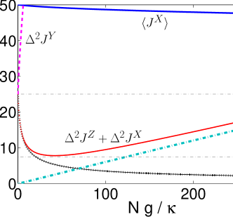
The best HZ entanglement (i.e. the smallest possible value for $E_{HZ}$) is given when the sum of the two variances of $J_{AB}^{X}$ and $J_{AB}^{Y}$ of (16) is minimized. As explained in Section III.D, this sum can never be zero.

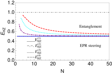
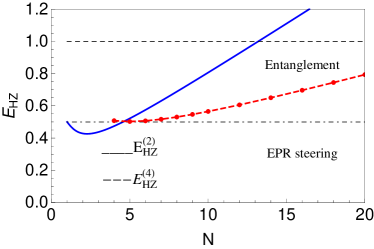
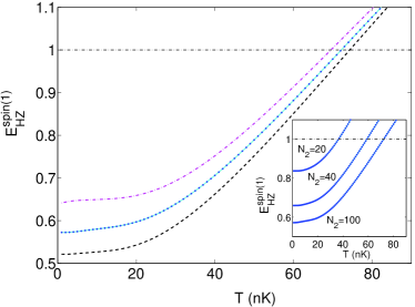
The best HZ inter-mode entanglement is achieved in the attractive regime ($g<0$) (as found in ${}^{41}K$ and ${}^{7}Li$ isotopes). The absolute lower bound for $E_{HZ}$ is predicted for the BEC ground state of (31) for a particular critical value $Ng_{11}/\kappa\approx-2.0$, as shown for $N=100$ in Fig. 7, and for $N=6$ in Fig. 8. This critical case has been studied and explained in cj and phase paper . We note however that the minimum $E_{HZ}$ becomes asymptotically small for large $N$. The maximum degree of HZ entanglement increases with $N$ the number of atoms, according to (18) and the relation for $C_{J}$ obtained in cj . The degree of entanglement is strong enough to give EPR steering.

We note that the strongest theoretical entropic entanglement $\varepsilon(\rho)$ entropy ; entropy2 is found for a pure state when all atom numbers are equally represented in the superposition. It is shown in bectheoryepr that the closest state to this optimum is obtained at a critical value of $Ng_{11}/\kappa\approx-2.0$, that is, the attractive interaction regime gives rise to a maximal spread in the distribution of numbers in each well.

Interestingly, Fig. 7 shows that the same point of maximum is observed for the higher order entanglement measure $E_{HZ}^{(2)}$. This measure can only detect entanglement that originates from superpositions of the type

$$|50\rangle|51\rangle+|51\rangle|50\rangle+|52\rangle|49\rangle$$

where at least some of the states of the superposition are separated by $2$ quanta (proved in Section III.B). Similarly, the third order entanglement criterion $E_{HZ}^{(3)}$ would detect entanglement originating from states separated by $3$ quanta. In the case of Fig 7, where there is $N=100$ quanta, the existence of entangled states such as $|0\rangle|100\rangle+...+|100\rangle|0\rangle$ could be detected in principle by measuring $E_{HZ}^{(100)}<1$. This would give a possible strategy for detecting the entanglement of the NOON state (the superposition $|N\rangle|0\rangle+|0\rangle|N\rangle$), though measurement of the higher order moments would present a challenge wellbecmurr . Higher order entanglement (e.g. $E_{HZ}^{(101)}<1$) would not be possible where the total number of atoms is fixed at $N$.

IV.2.2 Repulsive interactions

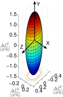
The repulsive regime of positive $g$ also predicts considerable planar squeezing and hence entanglement (Fig. 7), but, in that case, the best planar squeezing is rotated into the $X-Z$ plane as graphed in Fig. 9 phase paper ; guangzhou . A depiction of the resulting planar squeezing ellipsoid is shown in Fig 10.

Figure 9: (Color online) The repulsive interaction case for $N=100$, showing individual spin variances, and mean spin, $\langle J_{AB}^{X}\rangle$, for the ground state solution of Hamiltonian in the regime where there is a strong repulsive self-interaction $g/\kappa$, for $N=100$. Here $\kappa>0$ is fixed and $g$ is varied.

Thus, the corresponding HZ entanglement is between the modes defined by the rotated coordinates,

$$a^{\prime}=\left(a+b\right)/\left(\sqrt{2}i\right),\ b^{\prime}=\left(a-b\right)/\sqrt{2}.$$ (32)

Figure 10: (Color online) The 3-D variance ellipsoid corresponding to $N=100$ and a repulsive interaction at the optimum coupling of $Ng/\kappa=40$. Spin variances are reduced in both axes parallel to the $X-Z$ plane, to show strong, but not perfect, planar quantum squeezing. The variance increases perpendicular to the squeezing plane, along the $Y$ axis.

The corresponding entanglement criterion is given by:

$$0<E^{\prime}_{HZ}=\frac{\left(\Delta J_{AB}^{X}\right)^{2}+\left(\Delta J_{AB}^{Z}\right)^{2}}{\left(\langle a^{\dagger}a\rangle+\langle b^{\dagger}b\rangle\right)/2}\,.$$ (33)

The detection of spatial HZ entanglement between the two wells in the repulsive case would therefore require a different detection scheme, as proposed in phase paper . We note that in both repulsive and attractive cases, the HZ entanglement can be very significant, so that the EPR steering nonlocality Eq (LABEL:eq:eprsteerhz) is predicted via measurement of both the first and second order HZ moments. Figure 9 indicates that, for fixed $N$, the repulsive case shows an increasing and then reducing first order HZ entanglement (8), as the nonlinearity $g/\kappa$ increases. The optimum case for $N=100$ and a repulsive interaction occurs at a coupling of $Ng/\kappa=40$. The squeezing ellipsoid for this coupling is shown in Fig 10.

Figure 11: (Color online) Higher order entanglement for the case of $N=100$. Other parameters as in 7. The red dashed line shows a reduced $E_{HZ}$ entanglement as $g/\kappa$ is increased above a certain level. The solid black line (starred) shows the second order entanglement. Here $E_{HZ}^{(2)}<1$, indicating entanglement, is possible at higher $g/\kappa$ ratios where the first order (dashed) criterion shows no entanglement.

Interestingly, however, from Fig. 11, we see that the second order entanglement criterion for $N=100$ picks up more entanglement, suggestive that the drop in the entanglement measured by the first order criterion as the nonlinearity increases is due to a change in the nature of the entanglement $-$ that it involves superpositions of states with a greater number difference, as described in Section III.B $-$ rather than to a loss of entanglement itself. Fig. 8 shows that a similar behavior occurs at much lower particle numbers ($N=6$), although with less overall entanglement at the optimum coupling. In short, multiparticle entanglement is predicted detectable in the repulsive case for a wide range of parameter regimes.

We note that a second type of multiparticle entanglement can be inferred from the degree of first order entanglement. This approach was proposed in Ref. sorsolm and has been used to infer multiparticle entanglement in Bose Einstein condensates eprenthiedel ; Philipp2010 , based on measurements of the variance of $J_{AB}^{Z}$. This second type of multiparticle entanglement puts a constraint on the total number of particles in the entangled state, but can include states such as

$$\{|50\rangle|50\rangle+|49\rangle|51\rangle\}/\sqrt{2}$$

and is therefore different to that inferred from the higher order entanglement criteria involving $E_{HZ}^{(m)}$. Where the multiparticle entanglement is inferred from the first order variances, it is possible that the states making up the entanglement differ by only one particle number for each mode. More details for the HZ criterion will be given in a future paper.

IV.2.3 Comment on measurement schemes

The spatial inter-well entanglement can be confirmed, via $E_{HZ}$, from the measurements of the combined spins $J_{AB}$, using interference measurements between the two condensates, as has been performed in esteve . Results obtained in this fashion are important in confirming the existence of entanglement within quantum theory, but as the measurements are not localized at each site, they cannot be viewed as rigorous tests of EPR entanglement, steering or nonlocality. In order to use the above strategies to confirm an EPR-type entanglement, one would measure the local EPR observables, $X_{A/B}$ and $P_{A/B}$, at each well olsenferris ; neweprbec . This is because the moments of (4) are in terms of operators, $a$ and $b$, which are linear combinations of the hermitian observables, $X^{\prime}s$ and $P^{\prime}s$. Optically, the $X$ and $P$ are measured using phase sensitive local oscillators ou .

V EPR entanglement: Four component case

We examine in this section how to use two additional modes per site to perform an effective “local oscillator” measurement in this BEC case. Such strategies have been suggested by Ferris et al olsenferris .

V.1 Linear multimode case

Figure 12: (Color online) We consider pairs of Fock states transmitted through a beam splitter. Pair $a_{1}$, $b_{1}$ are coupled and become entangled, as do $a_{2}$, $b_{2}$.

We study the linear case first, to model a fixed number of atoms with a minimal BEC nonlinear self interaction. Suppose a Fock number state $|\psi_{in}\rangle=|N_{1}\rangle_{a_{in1}}|N_{2}\rangle_{a_{in2}}|0\rangle_{b_{in1}}|0\rangle_{b_{in2}}$ is incident on a beam splitter (Fig. 12), so that $N_{1}$ and $N_{2}$ are fixed, and modes within each pair $a_{1},\ b_{1}$ and $a_{2},\ b_{2}$ are coupled by the BS interaction, with $a_{1}$ and $a_{2}$ (and $b_{1}$, $b_{2}$) remaining uncoupled. Output modes $a_{1}$ and $b_{1}$ are number-conserved according to (2); as is pair $a_{2}$, $b_{2}$, and are given as $a_{1,2}=(a_{in1,2}+b_{in1,2})/\sqrt{2}$, and $b_{1,2}=(a_{in1,2}-b_{in1,2})/\sqrt{2}$. The output state is

$$|out\rangle = \sum_{n=0}^{N_{1}}\sum_{n^{\prime}=0}^{N_{2}}c_{n,n^{\prime}}|n\rangle_{a1}|n^{\prime}\rangle_{a2}|N_{1}-n\rangle_{b1}|N_{2}-n^{\prime}\rangle_{b2}$$

where $c_{n,n^{\prime}}=\sqrt{N_{1}!N_{2}!}/\sqrt{2^{N_{1}+N_{2}}n!(N_{1}-n)!n^{\prime}!(N_{2}-n^{\prime})!}$. We can evaluate moments, to obtain the prediction for the HZ spin criterion Eq. (23). Fig. 13 shows the result of varying $N_{1}$ for fixed $N_{2}=100$. The asymmetric case is favorable to detecting entanglement.

Figure 13: (Color online) The entanglement of pairs of Fock states transmitted through a beam splitter can be detected via criterion Eq. (23) for the asymmetric case where pair $a_{2}$ and $b_{2}$ have much greater numbers $N_{2}\gg N_{1}$ ($N_{2}=100$). Entanglement is confirmed if $E_{HZ}^{spin\,(1)}<1$.

Where the initial state is more complex, such as $|\psi_{in}\rangle=|N_{1}\rangle_{a_{in1}}|N_{2}\rangle_{a_{in2}}|N_{1}\rangle_{b_{in1}}|N_{2}\rangle_{b_{in2}}$, the output state will involve superpositions of only even numbers of atoms in the symmetric and antisymmetric modes, so that $\mid\langle J_{A}^{+}J_{B}^{-}\rangle\mid^{2}=\mid\langle a_{2}^{\dagger}a_{1}b_{2}b_{1}^{\dagger}\rangle\mid^{2}=0$. As in the case of Section IV.2, we would detect this entanglement using an appropriate second order spin criterion.

V.2 Nonlinear four component BEC case

We now consider the EPR entanglement that can be generated and measured when the modes interact to form the four-mode BEC ground state. We focus on set-ups that will enable the four mode case to produce an EPR entanglement that is the replica of the two-mode HZ entanglement, as displayed in Figures (7-11). In this case, the second mode at each site may be thought of as part of a measurement system (Fig. 2).

V.2.1 Four-mode BEC Hamiltonian

We assume the two-well, four-mode system of Fig 2 is described by the Hamiltonian fourmodecholsen :

$$\hat{H}/\hbar=\sum_{i}\kappa_{i}a_{i}^{\dagger}b_{i}+\frac{1}{2}\left[\sum_{ij}g_{ij}a_{i}^{\dagger}a_{j}^{\dagger}a_{j}a_{i}\right]+\left\{a_{i}\leftrightarrow b_{i}\right\}\,.$$ (35)

We solve for the ground state of this Hamiltonian. We consider two modes at each EPR site $A$ and $B$, with four modes in total, as shown schematically in Fig. 2. This corresponds to the two component per well experiments of Gross2010 , and somewhat less closely to the multi-mode interferometry experiments of Egorov . Depending on the exact configuration, the local modes at each EPR site can be independent (in which case local cross couplings $g_{ij}$ are zero ($g_{12}=0$)), or not independent, as would be the case where the modes are coupled by the BEC self interaction term, so the couplings cannot be “turned off”, as in the set-up of Gross2010 . The coupling constant is proportional to the three-dimensional S-wave scattering length, so that $g_{ij}\propto a_{ij}$, as in the two-mode case. For example, a typical value of the S-wave scattering length for ${}^{87}Rb$ is $a_{11}=100.4a_{0}$, where $a_{0}$ is a Bohr radius. Zero cross couplings are likely to require spatial separation of the two local modes, as might be achievable with four wells. The quantum dynamics of the four-well Bose Hubbard model has been studied recently with two different tunnelling rates fourmodecholsen .

The Hamiltonian (35) with $\kappa=\kappa_{1}=\kappa_{2}$ is based on the assumption that the second pair of modes $a_{2},b_{2}$ are coupled between the wells in the same way as the first pair $a_{1},b_{1}$, which implies similar diffusion across wells. The case where $\kappa_{2}=0$, $\kappa_{1}\neq 0$ is possible where diffusion across the wells can be controlled, as where the local modes represent separate wells. We will examine the predictions for both cases.

V.2.2 Symmetric tunneling case

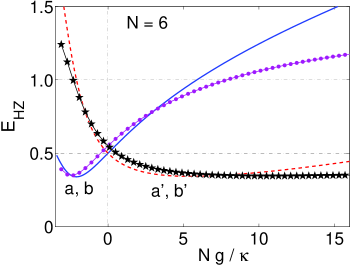
The BEC nonlinearity can enhance the entanglement. This is evident on comparing with the case of zero atom-atom interaction ($g_{ij}=0$), which corresponds to the result of the linear beamsplitter model (Fig. 12), and is indicated by the large red circles in the Figures 14-16. First, we examine the case of symmetric inter-well tunneling with $\kappa=\kappa_{1}=\kappa_{2}$, so there is complete symmetry between the nonlocal setups, but a variable local cross coupling $g_{12}$. Figure 14 shows entanglement using the HZ spin criterion Eq. (23), for the ground state, for cases of both zero and strong local couplings $g_{12}$. Asymmetric atom numbers with $N_{1}\ll N_{2}$ are required for the best entanglement, however, as shown in the inset of Fig. 14.

Figure 14: (Color online) Entanglement using adiabatic cooling to ground state in a two-well potential, at $T=0K$, for the four mode model of Fig. 2, with a variety of local cross couplings $g_{ij}$. Here $\kappa=\kappa_{1}=\kappa_{2}>0$ and $g_{11}$ is varied with the other values of $g_{ij}$ held in a fixed ratio, with $N_{1}=5,\ N_{2}=100$. $E_{HZ}^{spin\,(1)}<1$ indicates entanglement; $E_{HZ}^{spin\,(1)}<0.5$ indicates EPR steering. Curves are labelled in order of nesting as: (purple dash dotted) equal couplings; (blue dots) non-zero cross-couplings corresponding to ${}^{87}Rb$ Feshbach resonance with $a_{11}=100.4a_{0},\ a_{12}=80.8a_{0},\ a_{22}=95.5a_{0}$; (black dashed) without cross-correlations $g_{12}=0$; $g_{22}=g_{11}$; (green solid curve) negative relative cross-coupling $g_{11}.g_{12}<0$. The inset shows the effect of increasingly symmetric atom numbers.

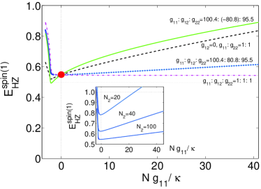
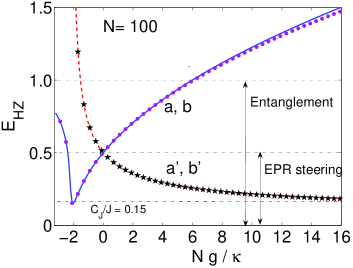
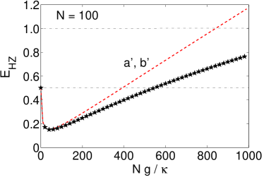
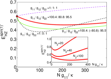
We note from Fig. 14 that the entanglement is improved by using a “local oscillator”-type approach, in which the second modes $a_{2}$, $b_{2}$ are independent of the first at each location ($g_{12}=0$) (being only combined at the spin measurement stage (19)) and are of much greater numbers ($N_{2}\gg N_{1}$) olsenferris ; eprenthiedel . In addition however, we note from the black dashed curve of Fig. 15 that better entanglement is obtained if the second “local oscillator” pair $a_{2}$, $b_{2}$ are also entangled optimally, as given by the critical point of the plots in Fig. 7. Thus, the optimal $E_{HZ}^{(1)}$ is at $N_{2}g_{22}/\kappa_{2}\approx-2.03$ for the modes $a_{2}$ and $b_{2}$, and at ${\color[rgb]{0,0,0}N_{1}g_{11}/\kappa_{1}\approx-2.1}$ for modes $a_{1}$ and $b_{1}$ (as shown in the inset of Fig. 15). The choice $N_{2}g_{22}\sim N_{1}g_{11}$ therefore gives enhanced EPR spin entanglement (red solid curve of Fig. 14).

The minimum of $E_{HZ}^{spin\,(1)}$ corresponds to the minimum achievable for the HZ entanglement $E_{HZ}^{(1)}$; this minimum is presented for the case $N_{1}=100$ in Fig. 7. Better entanglement is thus achieved by increasing the number of atoms $N_{1}$, provided the other constraints, that $N_{2}\gg N_{1}$ and $g_{11}$ and $g_{22}$ correspond to the critical choice for each mode pair, are satisfied, as shown in Fig. 15. Analytical details are given in the Appendix.

Figure 15: Entanglement using adiabatic cooling to ground state in a two-well potential, at $T=0K$. Here $\kappa=\kappa_{1}=\kappa_{2}$, $g_{12}=0$, and both $g_{11}$ and $g_{22}$ are varied so that $N_{1}g_{11}/\kappa_{1}=N_{2}g_{22}/\kappa_{2}$ . $E_{HZ}^{spin\,(1)}<1$ indicates entanglement; $E_{HZ}^{spin\,(1)}<0.5$ indicates EPR steering. Main graph: (black dashed curve) $N_{1}=5,\ N_{2}=100$; (blue dotted curve) $N_{1}=20$, $N_{2}=100$. The curves are for values of local coupling that optimize $E_{HZ}^{(1)}$ for each mode pair, in which case for $N_{2}\gg N_{1}$ the $E_{HZ}^{spin\,(1)}$ becomes the $E_{HZ}^{(1)}$ displayed in Fig. 7. The inset reveals the individual degree of HZ entanglement $E_{HZ}^{(1)}$ for the mode pairs $a_{1}$,$b_{1}$ and $a_{2}$,$b_{2}$, as explained in the text.

Figure 16: (Color online) Adiabatic cooling to ground state in a two-well potential, at $T=0K$. Here $\kappa=\kappa_{1}=\kappa_{2}$. Parameters are as for Fig. 14, but the entanglement parameter is calculated for the rotated modes $a^{\prime},\ b^{\prime}$ of Eq. (32). For large $N_{2}$, the strength of entanglement measure is enough to confirm EPR steering via the criterion Eq. (LABEL:eq:spinhzeprcritvar).

It is interesting that the case of approximately equal couplings $g_{11}=g_{22}=g_{12}$ is generally less favorable for the HZ spin entanglement (Figure 14). This can be understood if we rewrite the Hamiltonian (35) in terms of the spin operators. We obtain $H\simeq\chi\left(J_{A}^{Z}\right)^{2}+\chi\left(J_{B}^{Z}\right)^{2}+\kappa(a_{1}^{\dagger}b_{1}+a_{1}b_{1}^{\dagger}+a_{2}^{\dagger}b_{2}+a_{2}b_{2}^{\dagger})$, where $\chi\simeq\frac{1}{2}(g_{11}+g_{22}-2g_{12})$ gives the effective nonlinearity, and those terms related to $J_{A,B}^{Z},\ N_{1,2}^{2},\ N_{1,2}$ have been omitted. For equal couplings $g_{12}=g_{11}=g_{22}$, the Hamiltonian thus effectively reduces to the linear term of the BS model of Fig. 12, the predictions of which are given by the red circles in Figs 14 and 15. This is evident in the results of Figs. 14 and 15. Furthermore, enhancement of the nonlinearity is possible, if $g_{12}$ becomes negative. The green solid curve of Figure 14 shows an enhanced entanglement for negative local cross-coupling, $g_{12}<0$.

As is consistent with the two-mode results, the spin HZ entanglement is optimal in the attractive regime, $g_{11}<0$. Enhancement of entanglement in the repulsive regime is possible (Fig. 16), if one examines the spin HZ entanglement for the rotated modes, $a^{\prime},\ b^{\prime}$ of Eq. (32).

The effect of temperature is presented in Fig. 17. In our calculations, we account for finite temperatures by assuming a canonical ensemble of $\rho=\exp[-H/k_{B}T]$, with an inter-well coupling of $\kappa/k_{B}=50nK$. The critical temperature for the spin HZ entanglement signature is shown in Fig. 17.

V.2.3 Asymmetric tunneling case

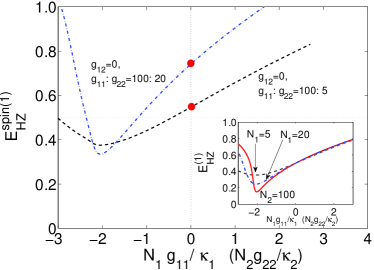
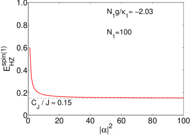
An alternative strategy more closely aligned to those used in optics is to consider $\kappa_{2}=0$ , $\kappa_{1}\neq 0$. In this case, the modes $a_{2}$ and $b_{2}$ are uncoupled and independent. If they are prepared in coherent states $|\alpha_{2}\rangle|\beta_{2}\rangle$ (we take $\alpha_{2}=\beta_{2}=\alpha$, where $\alpha$ is real), with $\alpha$ large, the entanglement $E_{HZ}^{spin\,(1)}$ approaches the value given in the two-mode case, by $E_{HZ}^{(1)}$. We explain this as follows. For independent modes, as shown by equation (LABEL:eq:simindephzspin-1) of the Appendix, the HZ spin entanglement criterion (20) becomes, upon assuming coherent states for $a_{2}$ and $b_{2}$,

$$|\langle a_{1}^{\dagger}b_{1}\rangle|^{2}\alpha^{4}>\langle a_{1}^{\dagger}a_{1}b_{1}^{\dagger}b_{1}\rangle(1+\alpha^{2})^{2}$$ (36)

which we see will approach the required two-mode entanglement level in the limit of large $\alpha$. Figure 18 plots the result with finite numbers of atoms for the case of optimal $E_{HZ}^{(1)}$ which occurs at $N_{1}g_{11}/\kappa_{1}\approx-2.03$ when $N_{1}=100$. We can see that the four mode EPR entanglement achieved ($C_{J}/J\approx 0.15$) is that of the two-mode case (Fig. 7) provided there is a large enough number of atoms in the second mode.

Figure 17: (Color online) The effect of critical temperatures corresponding to the parameters of Fig. 14 when $Ng/\kappa\approx-2.23$.

Figure 18: (Color online) The effect of an uncorrelated coherent atomic oscillator field for mode $2$ in a coherent state with amplitude $\alpha$, in the optimal case of Fig. 7 when $N_{1}g/\kappa\approx-2.03$.

VI Conclusion

We have examined strategies capable of generating detectable entanglement between two spatially-separated potential wells in a BEC. These include both two and four-mode strategies similar to those already used for spin-squeezing, but generalized to a double well. The model used to calculate the relevant variances has been shown to give a good fit to experimental data guangzhou ; Gross2010 . Our results find that local cross couplings can have a strong effect on entanglement, and results for the EPR entanglement improve with higher atom numbers. We find that a spin version of the Hillery-Zubairy (HZ) entanglement criterion appears readily suited to analyzing entanglement and the EPR steering paradox in these experiments. Furthermore, we have shown that the higher order HZ entanglement criteria can give information about the number of particles involved in the entangled state and the nature of the multiparticle entanglement.

The predictions in this paper are based on the assumption that the total number $N$ of atoms is fixed. Entanglement ($E_{HZ}^{(1)}=0.5$), though not EPR-steering, is obtainable between the output ports of a beam splitter with a number (Fock) state input, in the absence of nonlinear coupling terms, as was shown in Sections IV.A and V.A. However, for coherent state inputs, which have a Poissonian number distribution, this entanglement is not possible cohbs , and we draw the conclusion that number fluctuations will have an important effect on the entanglement. The effect of particle fluctuations on entanglement and precision measurement has been studied recently by Hyllus et al partiintnumberfluctuation and He et al bectheoryepr ; phase paper . However, we make the final note that these studies do not treat the EPR steering nonlocality.

Appendix

In this Appendix, we show we show how to directly “convert” the inter-well entanglement shown in Fig. 7 to an EPR entanglement, with the use of a “local oscillator”-type treatment which applies where two of the strong local modes are uncorrelated. This is the case of $g_{12}=0$, illustrated in Fig. 2.

Local oscillator measurements are achieved optically by combining a mode with a very strong coherent state ou . We can achieve something effectively equivalent to a “local oscillator” measurement, where the second pair of levels $a_{2}$, $b_{2}$ are much more heavily populated than levels $a_{1}$ and $b_{1}$, by assuming the second pair of modes are in an uncorrelated coherent state. We explain this as follows. Since $J_{A}^{+}=a_{1}^{\dagger}a_{2}$ and $J_{A}^{-}=a_{1}a_{2}^{\dagger}$ and $J_{B}^{+}=b_{1}^{\dagger}b_{2}$ and $J_{B}^{-}=b_{1}b_{2}^{\dagger}$ we can rewrite the criterion (20) in terms of the mode operator moments, for this special case, by the factorization that is justified for independent fields at each location. Thus,

$$|\langle J_{A}^{+}J_{B}^{-}\rangle|^{2}=|\langle a_{1}^{\dagger}b_{1}\rangle\langle a_{2}b_{2}^{\dagger}\rangle|^{2}\,,$$ (37)

and similarly

$$\langle(J_{A}^{+}J_{A}^{-})(J_{B}^{+}J_{B}^{-})\rangle=\langle a_{1}^{\dagger}a_{2}a_{1}a_{2}^{\dagger}b_{1}^{\dagger}b_{2}b_{1}b_{2}^{\dagger}\rangle\,.$$ (38)

The criterion (20) becomes

$$|\langle a_{1}^{\dagger}b_{1}\rangle|^{2}|\langle a_{2}b_{2}^{\dagger}\rangle|^{2} > \langle a_{1}^{\dagger}a_{1}b_{1}^{\dagger}b_{1}\rangle\langle(1+a_{2}^{\dagger}a_{2})(1+b_{2}^{\dagger}b_{2})\rangle$$

Clearly, since the inter-well entanglement studied in Section IV and summarized in Fig. 7 enables $|\langle a_{1}^{\dagger}b_{1}\rangle|^{2}>\langle a_{1}^{\dagger}a_{1}b_{1}^{\dagger}b_{1}\rangle$ via the HZ entanglement criterion, we will have (at least) the same level of four mode EPR entanglement, provided

$$|\langle a_{2}b_{2}^{\dagger}\rangle|^{2}\geq\langle(1+a_{2}^{\dagger}a_{2})(1+b_{2}^{\dagger}b_{2})\rangle.$$ (40)

In fact, the inequality would represent violation of the two-site version of the Bell inequality discussed in CFRD , which is not achievable for this system. However, it is still possible to optimize the EPR entanglement. This can be achieved in the following way. If the two modes $a_{2}$ and $b_{2}$ are also coupled via an inter-well interaction ($\kappa_{2}\neq 0$ in Fig. 2), to produce the ground state solution of Fig 9, then $E_{HZ}^{(1)}<1$ amounts to $|\langle a_{2}b_{2}^{\dagger}\rangle|^{2}>\langle a_{2}^{\dagger}a_{2}b_{2}^{\dagger}b_{2}\rangle$. The optimal $E_{HZ}^{(1)}$ is at $N_{2}g_{22}/\kappa_{2}\approx-2.03$, while for the modes $a_{1}$ and $a_{2}$, the optimal (LABEL:eq:simindephzspin-1) occurs for ${\color[rgb]{0,0,0}N_{1}g_{11}/\kappa_{1}\approx-2.1}$ (inset of Fig. 15). This choice gives enhanced EPR entanglement as shown in Fig. 14. Better entanglement is possible for this optimal choice, as the numbers are increased (Fig. 15).

References

- (1) A. Einstein, B. Podolsky and N. Rosen, Phys. Rev. 47, 777 (1935).
- (2) J. S. Bell, Physics 1, 195 (1965); J. F. Clauser, M. A. Horne, A. Shimony and R. A. Holt, Phys. Rev. Lett. 23, 880 (1969).
- (3) J. F. Clauser and A. Shimony, Rep. Prog. Phys. 41, 1881 (1978).
- (4) A. Aspect, P. Grangier and Gerard Roger, Phys. Rev. Lett. 49, 91 (1982); A. Aspect, J. Dalibard and G. Roger, Phys. Rev. Lett. 49, 1804 (1982).
- (5) P. G. Kwiat et al., Phys. Rev. Lett. 75, 4337 (1995); G. Weihs et al., ibid. 81, 5039 (1998); W. Tittel et al., ibid. 84, 4737 (2000).
- (6) Z. Y. Ou et al, Phys. Rev. Lett. 68, 3663 (1992).
- (7) M. D. Reid, et. al., Rev. Mod. Phys. 81, 1727 (2009).
- (8) M. D. Reid, Phys. Rev. A 40, 913 (1989).
- (9) C. Lee, Phys. Rev. Lett. 97, 150402 (2006). C. Lee et al, Front. Phys. 7, 109 (2012).
- (10) A. K. Ekert, Phys. Rev. Lett. 67, 661 (1991).
- (11) D. J. Wineland et al., Phys. Rev. A 50, 67 (1994).
- (12) M. J. Holland and K. Burnett, Phys. Rev. Lett. 71, 1355 (1993).
- (13) J. P. Dowling, Phys Rev A 57, 4736 (1998).
- (14) L. Pezze and A. Smerzi, Phys Rev. Lett. 102, 100401 (2009).
- (15) G. Y. Xiang et al., Nature photonics 5, 43, (2011).
- (16) T. Opatrny and G. Kurizki, Phys. Rev. Lett. 86, 3180 (2001); K.V. Kheruntsyan and P. D. Drummond, Phys. Rev. A 66, 031602(R) (2002); K. V. Kheruntsyan, M. K. Olsen and P. D. Drummond, Phys. Rev. Lett. 95, 150405 (2005).
- (17) A. A. Norrie, R. J. Ballagh, and C. W. Gardiner, Phys. Rev. Lett. 94, 040401 (2005); P. Deuar and Peter D. Drummond, Phys. Rev. Lett. 98, 120402 (2007).
- (18) A. J. Ferris, M. K. Olsen, E. G. Cavalcanti and M. J. Davis, Phys. Rev. A 78, 060104 (2008); A. J. Ferris, M. K. Olsen and M. J. Davis, Phys. Rev. A 79, 043634 (2009).
- (19) P. Milman, A. Keller, E. Charron and O. Atabek, Phys. Rev. Lett. 99, 130405 (2007); Magnus Ögren and K. V. Kheruntsyan, Phys. Rev. A 82, 013641 (2010).
- (20) C. Orzel, A. K. Tuchman, M. L. Fenselau, M. Yasuda and M. A. Kasevich, Science 291, 2386 (2001).
- (21) M. Greiner, C. A. Regal, J. T. Stewart and D. S. Jin, Phys. Rev. Lett. 94, 110401 (2005).
- (22) J.-C. Jaskula, et. al., Phys. Rev. Lett. 105, 190402 (2010); V. Krachmalnicoff, et. al., Phys. Rev. Lett. 104, 150402 (2010).
- (23) Robert Bücker, et. al., Nature Physics 7, 608–611 (2011).
- (24) C. Gross, H. Strobel, E. Nicklas, T. Zibold, N. Bar-Gill, G. Kurizki and M. K. Oberthaler, Nature 480, 219 ( 2011).
- (25) B. Lücke, et. al., Science 334, 773 (2011).
- (26) J. Esteve, et. al., Nature 455, 1216 (2008).
- (27) C. Gross, T. Zibold, E. Nicklas, J. Esteve and M. K. Oberthaler, Nature (London) 464, 1165 (2010).
- (28) M. F. Riedel, P. Böhi, Y. Li, T.W. Hänsch, A. Sinatra and P. Treutlein, Nature (London) 464, 1170 (2010).
- (29) M. Egorov, et. al., Phys. Rev. A 84, 021605 (2011).
- (30) N. Bar-Gill, et. al., Phys. Rev. Lett. 106, 120404 (2011).
- (31) Q. Y. He, et. al., Phys. Rev. Lett. 106, 120405 (2011).
- (32) E. Schroedinger, Naturwiss. 23, 807 (1935); Proc. Cambridge Philos. Soc. 31, 555 (1935); Proc. Cambridge Philos. Soc. 32, 446 (1936).
- (33) H. M. Wiseman, S. J. Jones and A. C. Doherty, Phys. Rev. Lett. 98, 140402 (2007).
- (34) S. J. Jones, H. M. Wiseman and A. C. Doherty, Phys. Rev. A 76, 052116 (2007).
- (35) D. J. Saunders, et al, Nature Physics 6, 845 (2010).
- (36) A. J. Bennett et al, arXiv: 1111.0739. D. Smith et al, arXiv:1111.0829. B. Wittmann et al, arXiv:1111.0760.
- (37) E. G. Cavalcanti, et al, Phys. Rev. A 80, 032112 (2009).
- (38) S. L. Midgley, A. J. Ferris, M. K. Olsen, Phys Rev A81, 022101 (2010).
- (39) E. G. Cavalcanti, et al, Phys. Rev. A 84, 032115 (2011).
- (40) L. M. Duan, G. Giedke, J. I. Cirac and P. Zoller, Phys. Rev. Lett. 84, 2722 (2000).
- (41) R. Simon, Phys. Rev. Lett. 84, 2726 (2000).
- (42) V. Giovannetti, S. Mancini, D. Vitali and P. Tombesi, Phys. Rev. A 67, 022320 (2003).
- (43) A. Peng and A. S. Parkins, Phys. Rev. A 65, 062323 (2002); Q. Y. He et al, Phys. Rev. A 79, 022310 (2009); Q. Y. He, et al, Optics Express 17, 9662 (2009).
- (44) B. L. Schumaker and C. M. Caves, Phys. Rev. A 31, 3093 (1985).
- (45) M. D. Reid and P. D. Drummond, Phys. Rev. Lett. 60, 2731 (1988).
- (46) A. Heidmann et al, Phys. Rev. Lett. 59, 2555 (1987).
- (47) A. S. Lane et al, Phys Rev Lett. 60, 1940 (1988); Phys. Rev. A, 38, 788 (1988).
- (48) R. E. Slusher, et al, Phys. Rev. Lett. 55, 2409 (1985). M. D. Reid and D. F. Walls, Phys. Rev. A 33, 4465 (1986).
- (49) J. I. Cirac, M. Lewenstein, K. Molmer and P. Zoller, Phys. Rev. A 57, 1208 (1998); G. Mazzarella, L. Salasnich, A. Parola and F. Toigo, Phys. Rev. A 83, 053607 (2011); C. Bodet, J. Estève, M. K. Oberthaler and T. Gasenzer, Phys. Rev. A 81, 063605 (2010).
- (50) G. J. Milburn, J. Corney, E. M. Wright and D. F. Walls, Phys. Rev. A 55, 4318 (1997).
- (51) T. J. Haigh, A. J. Ferris, and M. K. Olsen, Opt. Commun. 283, 3540 (2010).
- (52) J. Dunningham and K. Burnett, Journ. Modern Optics 48, 1837, (2001).
- (53) D. Gordon and C. M. Savage, Phys Rev A 59, 4623 (1999).
- (54) L. D. Carr, D. R. Dounas-Frazer and M. A. Garcia-March, Europhysics Lett. 90, 10005 (2010).
- (55) F. Gerbier, S. Fölling, A. Widera, O. Mandel, I. Bloch, Phys Rev. Lett. 96, 090401 (2006).
- (56) M. Hillery and M. S. Zubairy, Phys. Rev. Lett. 96, 050503 (2006).
- (57) E. G. Cavalcanti, C. J. Foster, M. D. Reid, and P. D. Drummond, Phys. Rev. Lett. 99, 210405 (2007).
- (58) Q. Sun, H. Nha, and M. S. Zubairy, Phys. Rev. A 80, 020101(R) (2009).
- (59) A. Salles et al, arXiv:1002.1893.
- (60) Q. Y. He et al, Phys Rev A 81, 062106 (2010).
- (61) C. V. Chianca and M. K. Olsen, arXiv: 1104.3655.
- (62) Q. Y. He, P. D. Drummond, and M. D. Reid, Phys. Rev. A 83, 032120 (2011).
- (63) Q. Y. He, Shi-Guo Peng, P. D. Drummond, and M. D. Reid, Phys. Rev. A 84, 022107 (2011).
- (64) A. S. Sorensen and K. Molmer, Phys. Rev. Lett. 86, 4431 (2001).
- (65) E. G. Cavalcanti and M D Reid, Phys. Rev. Lett. 97, 170405 (2006).
- (66) H. F. Hofmann and S. Takeuchi, Phys. Rev. A 68, 032103 (2003).
- (67) G. Toth, Phys. Rev. A 69, 052327 (2004).
- (68) M. Hillery, H. T. Dung, and J. Niset, Phys. Rev. A 80, 052335 (2009).
- (69) H. Zheng, H. T. Dung, and M. Hillery, Phys. Rev. A 81, 062311 (2010).
- (70) M. Hillery, H. T. Dung, and H. Zheng, Phys. Rev. A 81, 062322 (2010).
- (71) Q. Y. He, T. Vaughan, P. D. Drummond and M. D. Reid, to be published.
- (72) Andrew P. Hines, Ross H. McKenzie, and Gerard J. Milburn, Phys. Rev. A 67, 013609 (2003).
- (73) Q. Xie and W. Hai, Eur. Phys. J. D 39, 277 (2006).
- (74) C. V. Chianca and M. K. Olsen, arXiv:1101.0451
- (75) M. D. Reid, Q. Y. He, and P. D. Drummond, Front. Phys. 7, 72 (2012). Q. Y. He, et al, Front. Phys. 7, 16 (2012).
- (76) B. E. Salah, D. Stoler, and M. C. Teich, Phys Rev A 27, 360 (1983).
- (77) P. Hyllus, L. Pezze and A. Smerzi, arXiv: 1003.0649 (2010).