Adiabatic response for Lindblad dynamics
Abstract
We study the adiabatic response of open systems governed by Lindblad evolutions. In such systems, there is an ambiguity in the assignment of observables to fluxes (rates) such as velocities and currents. For the appropriate notion of flux, the formulas for the transport coefficients are simple and explicit and are governed by the parallel transport on the manifold of instantaneous stationary states. Among our results we show that the response coefficients of open systems, whose stationary states are projections, is given by the adiabatic curvature.
1 Introduction
We are interested in extending the theory of adiabatic response of quantum systems undergoing unitary evolution [10, 26] to open (quantum) systems governed by Lindblad evolutions. In particular, we are interested in a geometric interpretation of the response coefficients.
In open systems there is usually some choice in setting the boundary between the system and the bath. Setting the boundary fixes the tensor product structure . Choosing a boundary still leaves a residual ambiguity in observables. For example, given a joint Hamiltonian of the system and the bath, there is no unique way of assigning to an observable of the form describing the energy of the system alone.
Example 1 (Lamb shift).
The interaction of an atom with the photonic vacuum has two effects on the atom: It leads to decay and to “Lamb shift” of the energy levels. One can choose whether to incorporate the Lamb shift in the energy of the atom or in its interaction with the bath.
Additional ambiguity arises when considering the flux (rate) of an observable . Any assignment of system observables to joint observables is incompatible with dynamics, if the bath and the system interact. In fact it is generally impossible to satisfy both requirements and .
The ambiguity in fluxes is physical and plays a key role in this work. Consider, for example, damped harmonic motion. By Newton, the flux of the momentum is the total force. This force is related to two other forces in this problem:
The momentum flux can be determined from the trajectory of the particle; The spring force from the force acting on the spring anchor and the friction from the momentum transfer to the bath. All these forces have physical significance and are associated with different measurements. In this work we shall focus on observables that are the analog of the momentum flux. This point of view has been emphasized in the works of [8, 17].
We study open systems described by Lindbladians [14, 13, 18, 20]. This framework is usually viewed as giving a simplified, often effective, but approximate description, of the Hamiltonian dynamics of a system interacting with a bath [24, 15, 25, 2]. Model Lindbladians can be derived from a Hamiltonian in the “weak coupling limit” provided the bath is memory-less (Markovian) [3, 14]. However, it is also possible to view Lindbladians from a broader perspective, and this is the point of view we take in this work, namely as the infinitesimal generators of state preserving maps [14]. As such, they provide a natural description of general quantum evolutions, in their own right.
The Lindblad operator, denoted , is made of a self-adjoint representing the “energy” of the system and a collection of operators, , representing the coupling to the bath. The notion of “energy” is, as we have noted in Example 1, ambiguous and this is manifested in the non-uniqueness of . A choice will be called a gauge. Different gauges generate the same dynamics.
We shall consider parametrized Lindbladians, , where the (classical) parameters are viewed as controls. This means that are functions of the controls111The functional dependence of a super operator it is indicated by its subscript; that of an operator or a state by its argument.. is the control space, see Fig. 1.
The main focus of this work is the development of an adiabatic222The notion of adiabaticity is contingent on a gap condition, Assumption 2 below. response theory for the fluxes; Namely, observables of the form . This notion is gauge invariant (independent of the choice ). It turns out that the adiabatic response of such observables has several simplifying features.
A different perspective on the choice of observables comes from a gauge invariant formulation of the principle of virtual work. For isolated systems the principle of virtual work assigns the observable with the variation of the -th control . Since is gauge dependent in the Lindblad setting, formulating a gauge invariant notion of the principle of virtual work requires the joint variation .
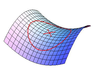
Consider a path in control space which is traversed adiabatically, Fig. 1. It is a feature of adiabatic evolutions [4] that stationary states evolve by parallel transport within the manifold of (instantaneous) stationary states. The response of fluxes is special in that it is fully determined by the parallel transport of the stationary states, (Theorem 9). This is the key to the geometric interpretation of the transport coefficients in linear response.
Parallel transport captures the geometric aspects of adiabatic evolution. However, as a practical method of calculation of transport coefficients, it suffers, in general, from its reliance on solving differential equations. A simplification occurs for (generic) Lindbladians where the (instantaneous) stationary state is unique and for dephasing Lindbladians (where the stationary states coincide with the eigenstates of the Hamiltonian [4]). In both cases parallel transport is determined algebraically, without recourse to solving differential equations. As a consequence, the transport coefficients are geometric and explicit.
In general, the response coefficients of open and closed systems are different. One would like to identify those transport coefficients that are immune to certain mechanism of decoherence and dephasing. For observables of the form the response coefficients depend on the manifold of stationary states (but not on the underlying dynamics). Immunity then follows whenever the stationary states are unaffected by decoherence and dephasing. This is the case for two physically interesting families of Lindbladians: Dephasing Lindbladians and Lindbladian which allow for decay to the (Hamiltonian) ground state.
2 Lindbladians
The Lindblad (super)333Super operators will be denoted by script characters. operator [14, 13] is given formally by444The normalization differs by factor 2 from that of [20].
| (1) |
where the state is trace class. The Hamiltonian part is self-adjoint (and local). The are essentially arbitrary, but finitely many for simplicity. Models describing exchange of energy involve non-self-adjoint while models of measurement involve which are spectral projections (non-local in general).
is the generator of state and trace preserving contractions. The dual (super) operator acts on the space of bounded operators, this being the dual of the space of trace class operators. When the evolution is unitary. To avoid technical difficulties with unbounded operators we shall assume:
Assumption 1.
and are bounded operators.
The assumption implies that a duality relation,
| (2) |
holds for all states and bounded operators . We shall occasionally consider standard physical examples with unbounded operators. However all these examples are simple enough that one can check that formal manipulations are indeed justified. We shall study the time evolution of the state :
| (3) |
It is convenient to introduce a notation that distinguishes stationary states from general states. We shall denote stationary states by , namely (with ). The (super) projection on the stationary states shall be denoted by , so .
2.1 Gauge transformations
does not determine . In fact, is invariant under the joint variation [13]
| (4) |
Moreover, and represent the same Lindbladian when is unitary in the sense that
| (5) |
We shall refer to the freedom in as gauge freedom. The observable , which one would like to interpret as the energy of the system, is therefore ambiguous a priori555Interferometry allows to compare the evolution in one arm of the interferometer with a different evolution in the other. This can be used to fix some of the gauge freedom. Interferometry for open system is described in [16]. . This ambiguity does not go away by considering explicit physical models weakly coupled to a bath, as Example 1 shows. In the examples that we consider, we pick a natural gauge.
2.2 Lindbladians with a unique stationary state
Generic finite dimensional Lindbladians have a unique stationary state . The (super) projections on the stationary state is given by
| (6) |
Evidently is trace preserving and (since ). It is not orthogonal, not even formally. In fact, the dual projection , which acts naturally on observables, is given by a different expression,
| (7) |
A basic identity we shall need is
| (8) |
The first equality is evident. The second follows from the trace preserving property of
We shall denote by the complementary projection
| (9) |
Evidently,
| (10) |
This will play a role in the sequel.
2.3 Dephasing Lindbladians
Dephasing Lindbladians are intermediate between Hamiltonians and Lindbladians with a unique stationary state. They are characterized 666When is simple, the characterization can be phrased as a commutation condition . The two characterizations differ e.g. in the case and the choice we make guarantees that dephasing Lindbladian share the stationary states with the Hamiltonian. by for some functions . In particular,
| (11) |
where is a spectral projection for .
When is finite dimensional, all spectral projections are finite dimensional and dephasing Lindbladians share the stationary states with the Hamiltonian. The manifold of stationary states is then the span of the . The (super) projections on this manifold and its complement , are given by
| (12) |
and are orthogonal projections, in the sense that their adjoints are given by the same expressions. satisfies Eq. (8) and satisfies Eq. (10).
3 Stationary states
Let us consider the (super) projections on the manifold of stationary states from a perspective that puts the special classes treated above in a uniform context.
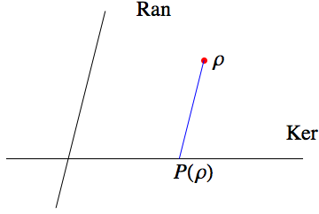
It is a basic property of Lindblad operators that kernel and range are transversal [4],
| (13) |
This follows from being a contraction: implies and we conclude .
This allows to define a projection on the direct sum by
| (14) |
Assumption 2 (Gap condition).
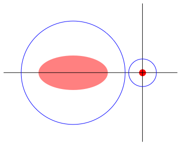
is an isolated point in the spectrum of and is given by the Riesz projection
| (15) |
where the contour encircles but no further points of the spectrum (see Fig. 3).
Remark 1.
If is an eigenvalue of finite algebraic multiplicity, then the Riesz projection part is for free. The assumption is satisfied when are finite dimensional. The assumption guarantees that is a closed subspace.
The consistency of Eqs. (14) and (15) deserves a discussion. In fact, the Riesz projection always satisfies the first line of Eq. (14) and the validity of the second one is the core of the assumption. To see this consider, besides of given by Eq. (15), also similarly given in terms of a contour encircling the complementary part of the spectrum. Then
| (16) |
proving the first line. Now assuming the second line of Eq. (14), the eigenspace associated to has a trivial Jordan block. This means that the Laurent expansion of the resolvent does not have a term and hence
| (17) |
and777We recall that is the Banach space notion of dual.
| (18) |
This places Eqs. (8, 10) into their general natural context.
Example 2 (Gapless Lindbladians).
It may happen that is gapped and is gapless. For example, let be a Hamiltonian with a ground state separated by a gap from a continuous spectrum. Then the associated Lindbladian has the eigenvalue 0 embedded in the continuous spectrum.
4 Controlled Lindbladians
The geometric aspects emerge when one turns one’s attention to a parametrized family of Lindbladians . We shall call the parameters control and the control space. This makes the Hamiltonian and the coupling to the bath functions of the controls. The explicit form of these functions is, of course, model specific.
Assumption 3 (Controlled Lindbladians).
-
(A)
The Lindbladian is a bounded (super) operator which is a smooth function of the controls .
-
(B)
The gap condition, Assumption 2, holds for all .
We shall call the stationary states of the instantaneous stationary states.
4.1 Iso-spectral Lindbladians
A distinguished family of controlled Lindbladians is the family of iso-spectral Lindbladians given by the action of unitaries on and :
| (19) |
The Lindbladian describing a harmonic oscillator coupled to a thermal bath, whose anchoring point is controlled, is an example:
Example 3 (Controlled oscillator in thermal contact).
A Harmonic oscillator, anchored at the origin and coupled to a heat bath, is described by the Lindbladian
| (20) |
and where . The stationary state of the oscillator is a thermal state with [13]. The Harmonic oscillator with controlled anchoring point is described by the iso-spectral family with . Explicitly
| (21) |
Since the ’s adjust to the oscillator wants to relax to the thermal state of the instantaneous Hamiltonian.
4.2 Parallel transport
We shall denote instantaneous stationary states by . By definition (we allow ). By Assumption 3 the projection on the stationary states, , is a smooth projection on control space and is a bounded operator valued form. For notational convenience, we henceforth suppress the explicit dependence and write for etc.
The differential of gives the identity . Since is a projection and consequently the projection is determined while is not. Parallel transport is the requirement, given in two equivalent forms,
| (22) |
This evolution of is naturally interpreted geometrically as parallel transport888For a different perspective which focuses on the analogs of Berry’s phase see e.g. [28]. : There is no motion in . The case is a special simple case, in that there is a unique state in the range of . It solves Eq. (22) without further ado.
Proposition 1.
The form is trace class.
4.3 Holonomy of parallel transport
In general, parallel transport, Eq. (22), does not integrate to a function on control space unless the curvature vanishes: (see Appendix B). If such a function exists, it will be called an integral of parallel transport. This is, of course, automatic if either , or , (see Eq. (6)).
Parallel transport is consistent with the convex structure of stationary states [4]. As a consequence it preserves extremal stationary states. Recall that a (stationary) state is called extremal if it can not be written as a convex combination of two other (stationary) states. For such extremal states we have:
Proposition 2 (Parallel transport of extremal states).
The parallel transport equation takes extremal stationary state to an extremal stationary state. If, moreover the manifold of (instantaneous) stationary states is a simplex, spanned by a finite number of isolated extremal states , then the function on
| (23) |
with independent of , is an integral of parallel transport.
Proof.
A more general statement has been proved in [4, Proposition 3]. The intuition is that states move inside as little as possible. In particular the boundary should be mapped by parallel transport to the boundary and extremal points to extremal points. ∎
Parallel transport is path independent for two important families of Lindbladians:
Finally we discuss the parallel transport for iso-spectral families.
Proposition 3.
The family is an integral of parallel transport, Eq. (22), if and only if
| (24) |
where . In particular the condition applies when is an isolated extremal point.
Proof.
5 Observables and fluxes
We denote observables by . The evolution of observables (in the Heisenberg representation) is generated by :
| (26) |
where
| (27) |
is itself an observable: We refer to either as the flux (or rate) of or simply as the flux . For example, the velocity is the flux of the position and the force is the flux of the momentum.
Assumption 4.
is not explicitly time dependent, i.e. , and hence .
Fluxes lie in . They have the special feature of vanishing expectation in stationary states. In fact:
Proposition 4 (No currents in stationary states).
Let be a trace class stationary state and the flux of the bounded observable . Then, . Conversely, if for any stationary state, then for some bounded observable .
Proof.
An example of an observable which is not a flux is:
Example 5 (Loop currents).
Consider a quantum particle on a ring with sites, , evolving by the (bounded) Hamiltonian
may be interpreted as the magnetic flux threading the ring. The stationary states are , (). The angular velocity is the (bounded) operator
Since does not vanish in stationary states, is not a flux: The angle is not an observable, since it is multivalued.
Current carrying stationary states can occur only when either the system is multiply connected or in the thermodynamic limit. Examples are supercurrents, where magnetic vortices effectively make the system multiply connected, and stationary currents in mesoscopic rings [11, 12]. The velocity is the flux of the position operator, which is usually unbounded. It is therefore interesting to examine conditions that would allow extending Prop. 4 to unbounded operators. Indeed, the gap condition implies that the expectation values of fluxes vanish in stationary states even for unbounded provided is bounded. Indeed, the gap condition allows us to use Eq. (18) and replace Eq. (28) by
| (30) |
A more careful discussion of this point is given in Prop. 16 of Appendix C.
An example where is unbounded but is bounded is:
Example 6 (Taming ).
Consider a quantum particle with spin hopping on the integer lattice. The Hilbert space is and let the Hamiltonian be
where is the unit left shift and and are the spin lowering and raising operators . Since we can write as a difference of two (infinite dimensional) projections:
The position operator is . It is clearly unbounded. Since , the velocity is the bounded operator
In fact, . The appropriate version of Eq. (12) says that is given by
being a product of bounded operators, it is bounded, even though is not.
5.1 Virtual work for Lindbladians
The principle of virtual work associates observables with variations of a controlled Hamiltonian . Our aim here is to formulate a corresponding principle for Lindbladians.
Observe that, first is a (super) operator, so its variation does not define an observable and second, the notion of “energy” is ambiguous in Lindblad evolutions. The principle of virtual work we formulate is gauge invariant in the sense of Section 2.1.
Theorem 5.
The observables given by
| (31) |
involving the joint variation of and , are (formally) self-adjoint and free from the ambiguity in and , under independent gauge transformations.
Proof.
Remark 2 (A second gauge invariant family).
A second family of observables that are gauge invariant is . This follows from the commutativity , and the unitarity of .
The observables extend the notion of the principle of virtual work to the Lindbladian setting. The physical interpretation of is often suggested by dimensional analysis. It depends on the choice of controls and is model dependent.
Example 7 (Controlled oscillator in thermal contact: Example 3 continued).
Shifting the anchoring point of the oscillator gives
is the spring force, while gives the friction force due to the cold contact and the gain from the hot contact. The observable distinguished by virtual work is the total force i.e. the momentum flux
| (32) |
In the example, the principle of virtual work gives a flux. This is not a coincidence. For iso-spectral Lindbladians, Eq. (19), virtual work is a flux. More precisely, let denote the (local) infinitesimal generators
| (33) |
(summation implied). The variations are:
| (34) |
Theorem 6 (Virtual work and fluxes).
For iso-spectral families of Lindbladians generated by , the observables associated with the principle of virtual work, Eq. (31), are the fluxes of the generators :
| (35) |
In particular we have Noether’s theorem in the form: If is a symmetry, in the sense that the r.h.s. vanishes, then its generator is a conserved quantity.
5.2 Currents
Just as there are three notions of force in a damped oscillator, there are several notions of currents in an open system. By partitioning the the system into a subsystem and its complement , one identifies three notions of currents:
-
•
The rate of charge in the subsystem ,
(36) -
•
For charge conserving , i.e. , the current flowing from to its complement is
(37) With local, this current is naturally associated with the boundary.
-
•
The current, , flowing from the subsystem to the bath defined via charge conservation
(38)
The three currents are measured by different instruments: is measured by an electrometer while is measured by an ammeter that monitors the flow at the boundary between the subsystems. In view of
| (39) |
The partitioning of into and is, of course, gauge dependent. Models often offer a natural choice of .
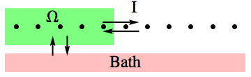
Example 8.
Consider Fermions hopping on a one dimensional lattice which can also tunnel in and out of a bath. The Lindbladian has
with the usual Fermion annihilation operators for site . The charge in the left semi-infinite box is
and the currents in Eq. (38) are
is localized at the boundary of the box, whereas is not.
In appendix A we elaborate on the notion of currents in magentic fields and in particular, describe the current densities in a model for the open quantum Hall system. We find three current densities: A Hamiltonian current density, a diffusion current and a dissipative chiral current.
6 Adiabatic Response
We are interested in adiabatically changing controls; where is the slow time. The evolution equation for the state is
| (40) |
with initial state that is an instantaneous stationary state999The general case, where the initial state is not a stationary state, is different and more complicated, because Eq. (13) has no analog. It is treated in e.g. [23]. . The adiabatic time scale is the largest time scale in the problem and the adiabatic limit is governed by the stationary states of . Another natural, limit, studied in [15, 21], lets the dissipation time scale increase with the adiabatic time scale. This limit is governed by the stationary states of rather than those of .
A key feature of adiabatic theory is that the evolution of is slaved to the evolution of . We borrow from [4]:
Proposition 7 (Adiabatic evolution).
The solution of Eq. (40) with initial condition the stationary state is
| (41) |
and
| (42) |
where is the corresponding integral of parallel transport.
is well defined and bounded since . This follows from parallel transport and the definition of as the projection on .
6.1 The response of unique stationary states
We are interested in the response of the observable of an adiabatically driven system. The case of a unique stationary state is simpler than the general case and we treat it first.
Proposition 8 (Response coefficients).
Suppose that the stationary state is unique. Let be a bounded observable and a solution of the adiabatic Lindblad evolution, Eq. (40), with initial state a normalized stationary state . Then, the response at slow time is memory-less and is given by
(summation implied) with the instantaneous stationary state and . The response coefficients
| (43) |
are functions on control space .
Proof.
The first term is of , and describes the persistent response, a property of the stationary state. The second term is the driven response which is proportional to the driving , the (unscaled) velocity of the controls.
One is often interested in situations where is constant on . This feature depends on additional structure (e.g. thermodynamic limit, disorder [9, 6, 1]). Observe that the expression for involves inverting , an operator with a non-trivial kernel, and so is not completely elementary.
Remark 3.
The formula for the response coefficient can be cast in a way that is formally reminiscent of Kubo’s formula:
When the manifold of stationary states is multidimensional, the persistent response has memory and can not be viewed anymore as functions on control space (see Section 4.3).
7 Response of fluxes
In the case of observable which are fluxes several simplifications occur: There is no persistent response and the formula for simplifies and becomes elementary. If, in addition, the extremal stationary states are isolated (Section 4.3) then, in addition, defines a function on .
By definition, a flux (which is not explicitly time dependent, Assumption 4) can be written as
| (44) |
where the replacement by relies on Eq. (18) and is only of interest in the infinite dimensional case where is unbounded while is bounded.
Theorem 9 (Response of fluxes).
Suppose that is an integral of parallel transport and that the flux and are bounded operators. Then, to leading order, the response is memory-less, linear in the driving and given by
(summation implied) and where the response coefficient
is a function on .
The observation that one can sometimes avoid computing Green functions in linear response is at the heart of the TKNN formula for the Hall conductance [27].
7.1 Geometric magnetism for iso-spectral families
The response coefficients of an iso-spectral family generated by are naturally organized as a matrix , relating the response of the flux of to the driving . The analog of the formula in Prop. 8 is
Combining Theorem 9 and Eq. (25) we get for the response matrix
| (45) |
We are now ready to state our main result:
Theorem 10 (Geometric response).
Suppose are bounded and is an integral of parallel transport. Then the response matrix is antisymmetric and given by
| (46) |
If, moreover, is a projection then is the adiabatic curvature of the bundle (see Appendix B):
| (47) |
For unitary evolutions, the first part of the theorem reduces to a (special case of) result of Berry and Robbins [10], who coined the term geometric magnetism for the anti-symmetric part of .
The second part of Theorem 10 extends the geometric interpretation of response matrix from the unitary case [7] to open systems. The conditions in the theorem are satisfied for Lindbladians representing relaxation to the ground state and dephasing Lindbladians whose initial state is a spectral projection.
Proof.
The conditions have been set so that the formal manipulations are justified
where in the second equality we used Eq. (25).
For the second part observe that the equation implies
Hence
where the first line is a readily checked identity. ∎
Remark 4.
More details about the dephasing case are in Appendix B where a formula for response when is not the integral of parallel transport is given.
In may happen that is proportional to the identity. The transport coefficients are then purely geometric and independent of the dynamics. An example is the Hall mobility:
Example 9 (Hall mobility).
The Landau Lindbladian, (see Eqs. (53) and (54) of Appendix A) is a model of a quantum particle in two dimensions, moving under the influence of a uniform, perpendicular, magnetic field, , in contact with a thermal bath. The corresponding controlled Lindbladian is the iso-spectral family generated by
The virtual work associated with the variation of the controls is, as explained in Appendix A, the velocity , while is interpreted as an electric field. The transport coefficient relating velocity to field strength is the mobility, given by
| (48) |
and independent of and the stationary state101010 The Landau Lindbladian in the plane has . One can avoid this by considering the model on the torus (with appropriate boundary conditions)..
By extension the model describes a gas of independent particles of density and conductance . If the density corresponds to filling factor 1, i.e. to one particle per unit magnetic flux, then , and the conductance is quantized in the same units as in the unitary case.
Remark 5 (Hall viscosity).
Theorem 10 can be used to recover, and generalize, results of Read and Rezayi [22] on the Hall viscosity: viscosity is the study of the Landau Lindbladian under the iso-spectral family generated by shears. The commutator of shears in two dimensions is the generators of rotation. Theorem 10 then relates the Hall viscosity with the expectation of the angular momentum per particle.
7.2 Friction and dissipation
The fact that of Eq. (46) is anti-symmetric does not imply the absence of dissipation. It only says that looking at the response of fluxes is not appropriate for the study of dissipation. To explain this statement consider the dissipation associated with the dragging of the anchoring point of a (damped) oscillator coupled to a heat bath at velocity . The response coefficient relating force to velocity is friction. As there are three forces in the problem—the momentum rate, the force on the anchoring point, and the friction force—there are also three friction coefficients. The friction coefficient associated with the momentum rate vanishes, but the others do not.
Example 10 (Friction: Example 7 continued).
The (unbounded) generator of shifts is, . With a thermal state of the oscillator, is trace class and Eq. (46) applies with . The friction coefficient vanishes, as it must by anti-symmetry.
The momentum rate vanishes because it can not disentangle the heat lost to the bath from the mechanical work done by the anchoring point. To study dissipation it is not enough to look at the response coefficients of fluxes, nor is it enough to examine the energy of the system.
Indeed, the energy of the (small) system, in the adiabatic limit, is
| (49) |
by Eq. (41). In particular, for an iso-spectral family the energy is constant (to leading order) when and undergo the same unitary transformation, as is the case in the example of the damped oscillator. The energy does not reveal the dissipation.
To reveal the dissipation one needs to look at the breakup of the energy to work and heat. The variation of the energy
| (50) |
expresses the first law of thermodynamics [25]
To compute the friction one needs to study the expectation of the spring force rather than the momentum flux . (More generally, rather than the flux of Eq. (35).)
In general, the computation of is complicated for two reasons: First, one needs to evaluate . Second, in the case that the ground state is non-unique, it also needs the explicit expression for the term in the adiabatic expansion, Eq. (41), which are history dependent. For dephasing Lindbladian such a computation is given in [5]. We shall not pursue this direction here.
8 Concluding remarks
We have derived a simple and general formulas for the adiabatic response coefficients for observable of the form . In the case of iso-spectral families of Lindbladians, the response matrix is determined by geometry and is purely anti-symmetric. We find a range of circumstances where the response coefficients are given by the adiabatic curvature of the associated stationary projections. It will be interesting to extend the theory to models of extended systems with (non-interacting) fermions.
Acknowledgments. JEA is supported by the ISF, the NSF under Grant No. PHY11-25915 and the fund for promotion of research at the Technion. MF was supported by UNESCO and ISF. We thank M. Porta for useful discussions.
Appendix A Currents in a magnetic field
The action of a magnetic field on charged particles endows the dynamics with chirality. This has interesting consequences for currents. Consider the Lindbladian describing a charged particle in the plane under the influence of a constant magnetic field coupled to a heat bath. The Hamiltonian is the Landau Hamiltonian
| (53) |
and the thermal bath is represented by (cf. Example 3)
| (54) |
We shall call the generator of the corresponding evolution a thermal Landau Lindbladian. The model has a current density associated to the total current Eq. (38).
Proposition 11.
Before proving the statement, let us comment about its content. By Eq. (56) the total current is unique up to a curl. The Hamiltonian current is proportional and parallel to the velocity . The dissipative current has a (non-chiral) diffusive term proportional to the gradient of the density and a further chiral term. The dissipative currents can be interpreted in terms of Brownian motion (see below).
Proof.
The dissipative terms of the Lindbladian are
For a function of position we have
| (57) |
Eq. (39) then gives the dual form of the statements of the proposition, namely,
∎
A.1 Stochastic interpretation
The dissipative currents admit an interpretation in terms of a (classical) stochastic process. To see this note first that for functions of either velocity ()
| (58) |
which can be read as if originating from a (exciting or damping) Langevin equation
where is a Brownian motion with zero drift and variance
In fact, expanding to first order in and to second order in yields that expression.
To derive the Langevin equation for we first note that the guiding center ,
| (59) |
satisfies and thus is a constant of motion for the Lindbladian, . Insisting on being a constant of motion, we have
| (60) |
In view of this is the Langevin equation corresponding to Eq. (57). (Beware: .) We can now combine with Theorem 6 to conclude
Proposition 12 (Velocity as virtual work).
The (negative) virtual work associated with the variation of the iso-spectral family of Landau Lindbladians generated by
| (61) |
is the velocity .
is the generator of the unitary family given by
| (62) |
The physical interpretation of the controls emerges by noting that
| (63) |
Since appears in like a pure gauge field, its variation in time, is a constant electric field that drives the system.
Remark 6 (Gauge covariance).
The proposition may be viewed as a manifestation of gauge and translation covariance, in the sense that and appear in the Lindbladian only through the minimal coupling expression . The virtual work associated with the variations generated by is the same as the variation generated by . This follows from
in fact both sides equal .
Appendix B Geometry of projections
Consider continuous orthogonal projections with . The superprojection that takes to is, Eq. (12),
We are going to describe parallel transport inside [19].
For a given path , parallel transport maps vectors in the range of to vectors in that of . That map is unitary and generated by
| (64) |
In fact , since , and, for so defined, satisfies
as required. And for the parallel transport equation (22), , holds true.
When , the parallel transport is manifestly path independent. In general, this is determined by the standard condition of vanishing curvature:
Proposition 13.
Let be an operator valued 1-form. The differential equation
admits a (locally path independent) solution if and only if the curvature vanishes
| (65) |
It implies the following criterion for the case of parallel transport of projections.
Proposition 14 (Adiabatic curvature).
The parallel transport constructed above is locally path independent if and only if the adiabatic curvature
commutes with all elements in .
Proof.
Parallel transport of a vector in the range of along an infinitesimal square maps
The associated adjoint transformation maps the state as
This allows to read off the curvature of seen in Eq. (65): By we have
Hence the criterion of vanishing curvature states that commutes with all elements in .
Computation gives the commutator
| (66) |
as the sum of adiabatic curvatures of all the spectral projections. Since
one finds
∎
For an iso-spectral family of projections
the generator of parallel transport, Eq. (64), is
since by Eq. (12). While it does not coincide with it differs from it only inside
| (67) |
When and the parallel transport can not be integrated in general. And the response coefficients are not functions on the manifold.
Theorem 15.
Suppose are bounded and is a dephasing Lindbladian. Then the response associated to the driving path and flux depends only on the integral of parallel transport and the derivative at the end point,
where
Proof.
Example 11 (Taming : Example 6 continued).
Consider a family of Hamiltonians generated by a momentum shift
where is the position operator. The generator of the parallel transport is
Although , their difference commutes with the Hamiltonian. Furthermore intertwines ,
which is equivalent to the statement that generates no motion inside , .
Appendix C Currents and unbounded observables
We discuss the precise meaning of Eq. (30) when is unbounded. We still assume that and are bounded, while need not be. Yet, the commutators and , defined as quadratic forms on the domain of , are assumed bounded, and . Then is a bounded operator by natural interpretation of Eq. (26) in the sense of quadratic forms.
Proposition 16.
Under the stated conditions, for any (trace class) stationary state . Moreover, is well-defined as a bounded operator. It is given as a strong limit, , by means of any sequence of bounded approximants with , (); finally .
Proof.
There exist sequences as stated, e.g. . The assumption states that the bounded operator is characterized by the property
| (68) |
Hence (weakly), and similarly for . Thus (weakly). Using that (weakly) and trace class imply , we conclude
| (69) |
by Eq. (28). Moreover, by Eq. (18) we have . We notice that is weakly continuous, and so are and the inverse of on , i.e.
| (70) |
in the notation of Eq. (15). As a result is weakly convergent to a limit denoted , and the result follows. ∎
References
- [1] M. Aizenman and G.M. Graf. Localization bounds for an electron gas. Journal of Physics A: Mathematical and General, 31(32):6783–6806, 1998.
- [2] W. Aschbacher, V. Jaksic, Y. Pautrat, and C.-A. Pillet. Topics in non-equilibrium quantum statistical mechanics. In S. Attal, A. Joye, and C.-A. Pillet, editors, Open Quantum Systems III, volume 1882 of Lecture Notes in Mathematics, pages 1–66. Springer Berlin / Heidelberg, 2006.
- [3] S. Attal, A. Joye, and C.-A. Pillet. Open Quantum Systems: The Markovian Approach. Springer, 2006.
- [4] J.E. Avron, M. Fraas, G.M. Graf, and P. Grech. Adiabatic theorems for generators of contracting evolutions. ArXiv e-prints, June 2011.
- [5] J.E. Avron, M. Fraas, G.M. Graf, and O. Kenneth. Quantum response of dephasing open systems. New Journal of Physics, and arXiv:1008.4079, 13:053042, 2011.
- [6] J.E. Avron, R. Seiler, and B. Simon. Quantum Hall effect and the relative index for projections. Phys. Rev. Lett., 65(17):2185–2188, Oct 1990.
- [7] J.E. Avron, R. Seiler, and L.G. Yaffe. Adiabatic theorems and applications to the quantum Hall effect. Comm. Math. Phys., 110:33–49, 1987.
- [8] J. Bellissard. Coherent and dissipative transport in aperiodic solids: An overview. Lecture Notes in Physics, pages 413–485, 2002.
- [9] J. Bellissard, A. van Elst, and H. Schulz-Baldes. The noncommutative geometry of the quantum Hall effect. J. Math. Phys., 35(10):5373–5451, 1994.
- [10] M.V. Berry and J.M. Robbins. Chaotic classical and half-classical adiabatic reactions: geometric magnetism and deterministic friction. Proc. R. Soc. Lond. A, 442:659–672, 1993.
- [11] F. Bloch. Flux quantization and dimensionality. Phys. Rev., 166:415–423, 1968.
- [12] D. Bohm. Note on a theorem of Bloch concerning possible causes of superconductivity. Phys. Rev., 75(3):502–504, 1949.
- [13] H.-P. Breuer and F. Petruccione. The Theory of Open Quantum Systems. Oxford University Press, USA, 2007.
- [14] E.B. Davies. Quantum theory of open systems. Academic Press [Harcourt Brace Jovanovich Publishers], London, 1976.
- [15] E.B. Davies and H. Spohn. Open quantum systems with time-dependent Hamiltonians and their linear response. J. Stat. Phys., 19:511–523, 1978.
- [16] M. Ericsson, E. Sjöqvist, J. Brännlund, D.K.L. Oi, and A.K. Pati. Generalization of the geometric phase to completely positive maps. Phys. Rev. A, 67:020101, Feb 2003.
- [17] R. Gebauer and R. Car. Current in open quantum systems. Phys. Rev. Lett., 93(16):160404, 2004.
- [18] V. Gorini, A. Kossakowski, and E.C.G. Sudarshan. Completely positive dynamical semigroups of -level systems. J. Math. Phys., 17(5):821–825, 1976.
- [19] T. Kato. On the adiabatic theorem of quantum mechanics. J. Phys. Soc. Japan, 5:435–439, 1950.
- [20] G. Lindblad. On the generators of quantum dynamical semigroups. Comm. Math. Phys., 48:119–130, 1976.
- [21] J.P. Pekola, V. Brosco, M. Möttönen, P. Solinas, and A. Shnirman. Decoherence in adiabatic quantum evolution: Application to Cooper pair pumping. Phys. Rev. Lett., 105:030401, Jul 2010.
- [22] N. Read and E.H. Rezayi. Hall viscosity, orbital spin, and geometry: paired superfluids and quantum Hall systems. ArXiv e-prints, August 2010.
- [23] M.S. Sarandy and D.A. Lidar. Adiabatic approximation in open quantum systems. Phys. Rev. A, 71:012331, Jan 2005.
- [24] H. Spohn. Large scale dynamics of interacting particles. Texts and Monographs in Physics. Springer-Verlag, 1991.
- [25] H. Spohn and J.L. Lebowitz. Irreversible thermodynamics for quantum systems weakly coupled to thermal reservoirs. Adv. Chem. Phys., 38:109–142, 1978.
- [26] D.J. Thouless. Quantization of particle transport. Phys. Rev. B, 27(10):6083–6087, 1983.
- [27] D.J. Thouless, M. Kohmoto, M.P. Nightingale, and M. den Nijs. Quantized Hall conductance in a two-dimensional periodic potential. Phys. Rev. Lett., 49(6):405–408, Aug 1982.
- [28] Robert S. Whitney, Yuriy Makhlin, Alexander Shnirman, and Yuval Gefen. Geometric nature of the environment-induced berry phase and geometric dephasing. Phys. Rev. Lett., 94:070407, Feb 2005.