Quantum Anomalous Hall Effect in Flat Band Ferromagnet

Abstract

We proposed a theory of quantum anomalous Hall effect in a flat-band ferromagnet on a two-dimensional (2D) decorated lattice with spin-orbit coupling. Free electrons on the lattice have dispersionless flat bands, and the ground state is highly degenerate when each lattice site is occupied averagely by one electron, i.e., the system is at half filling. The on-site Coulomb interaction can remove the degeneracy and give rise to the ferrimagnetism, which is the coexistence of the ferromagnetic and antiferromagnetic long-range orders. On the other hand the spin-orbit coupling makes the band structure topologically non-trivial, and produces the quantum spin Hall effect with a pair of helical edge states around the system boundary. Based on the rigorous results for the Hubbard model, we found that the Coulomb interaction can provide an effective staggered potential and turn the quantum spin Hall phase into a quantum anomalous Hall phase.

I INTRODUCTION

Quantum anomalous Hall effect (QAHE) is a quantum mechanical version of the Hall effect in a ferromagnet in absence of an external magnetic field or Landau levels. Different from the quantum Hall effect in a strong magnetic field, it originates from the topological properties of band structure in solid. Usually the anomalous Hall effect occurs in ferromagnetic metals due to the intrinsic spin-orbit coupling or extrinsic spin-orbit scattering.Sinova-10RMP It has been realized that the Hall conductance can be expressed as the summation of the Berry curvature in momentum space over all occupied states of electrons. This makes it possible to realize the quantum Hall effect even without the Landau levels.Haldane-88PRL A simple picture for QAHE was proposed in a two-dimensional electron gas with strong spin-orbit coupling.Qi-08PRB Electron localization in disordered systems also provides an alternative approach to realize this effect.Nagaosa-03PRL ; Li-09PRL The discovery of the quantum spin Hall effect (QSHE) and topological insulatorsKane-05PRL ; Kane-06PRB ; Zhang-06Science ; Konig-07Science ; Kane-07PRL ; Zhang-09Nature ; Zhang-09Science stimulated extensive interest to search QAHE in realistic systems. As a result of time-reversal symmetry breaking in topological insulators, this effect was predicted in a magnetically doped Hg_1-yMn_yTe quantum wellLiu-08PRL and Cr or Fe doped topological insulators,Yu-10Science in which the presence of magnetization suppresses one of helical edge states in QSHE, and preserves a chiral edge state for the quantum Hall effect. Very recently HgCr₂Se₄ is proposed to be a Chern semimetal and exhibits QAHE in quantum-well structure.Zhong-11PRL Interaction-driven topologically non-trivial Mott insulating phase displaying QAHE or QSHE has also attracted much research interest.Raghu-08PRL ; Ran-09PRB ; Sun-09RPL

While in search of ferromagnetism in diluted magnetic semiconductors, rigorous models of ferromagnetismTasaki-92PRL ; Mielke-93CMP or ferrimagnetism Lieb-89PRL ; Shen-94PRL in strongly correlated electron systems provides an alternative context to realize ferromagnetism. A common feature of these examples is the flat or almost flat band of electrons. The Coulomb interaction may remove high degeneracy of electrons in the band, leading to the ferromagnetism according to the Stoner criteria. Recently it was predicted that the ferromagnetism may occur in the Hubbard model with topological non-trivial bands.Katsura-10EPL

In this paper we propose a theory of QAHE in a flat band ferromagnet with spin-orbit coupling. We start with a two-dimensional decorated lattice model, which has a pair of flat bands in the middle of the energy spectrum. The inclusion of spin-orbit coupling makes the energy bands topologically non-trivial, and gives rise to QSHE. Based on the rigorous results for the Hubbard model, the Coulomb interaction may induce the ferrimagnetism in the ground state, when the middle flat bands are half filled. It provides an ideal way to realize a magnetic staggered field. The staggered field can modulate the topological numbers of electron bands by closing and reopening the energy gap.Chu-10PRB Different configurations of topological invariants assigned to the electron bands can then be obtained and will give different topological phases. Based on a self-consistent mean field calculation, we present the phase diagram of the ground state. We find that QAHE with nonzero Chern number can be realized in a ferromagnet due to the Coulomb interaction.

II A DECORATED LATTICE MODEL

We begin with the tight-binding Hamiltonian on a two-dimensional decorated lattice [see Fig. 1(a)],

$$\mathcal{H}=\mathcal{H}_{0}+\mathcal{H}_{SO},$$ (1)

where the spin-independent hopping term is given by

$$\mathcal{H}_{0}=t\sum_{\langle i,j\rangle}c_{i}^{\dagger}c_{j},$$

$c_{i}=(c_{i,\uparrow},c_{i,\downarrow})^{\mathrm{T}}$ and $c_{i,\uparrow(\downarrow)}^{\dagger}$ are the annihilation and creation operators of electron with spin $\uparrow(\downarrow)$ on site $i$. $\left\langle i,j\right\rangle$ means the summation over the nearest-neighbor sites. $t$ is the hopping amplitude. The spin-orbit coupling term has the form

$$\mathcal{H}_{SO}=\,\mathrm{i}\,\lambda\sum_{i\in\mathbb{A}}\sum_{j,l\in\mathbb{B}}c_{j}^{\dagger}\left[(\mathbf{d}_{ij}\times\mathbf{d}_{il})\cdot\mbox{\boldmath$\sigma$}\right]c_{l},$$

which gives a spin-dependent hopping between the next-nearest-neighbor sites with hopping amplitude $\lambda$ [shown by the dash lines in Fig. 1(a)]. Here the lattice is divided into two sublattices, $\mathbb{A}$ and $\mathbb{B}$, shown by the light and dark dots in Fig. 1(a), respectively. $j$ and $l$ denote the adjacent sites of site $i$, and $\mathbf{d}_{ij}$ is the unit vector along the direction from site $i$ to site $j$, and $\sigma$ are the Pauli matrices.

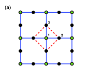
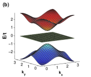
Figure 1: (Color online) (a) A two-dimensional decorated lattice. Dashed lines represent the hopping with spin-orbit coupling. The light (green) and dark (black) dots denote the sublattices $\mathbb{A}$ and $\mathbb{B}$, respectively. (b) The energy dispersion for $\mathcal{H}(\mathbf{k})$, which has three pairs of doubly degenerate bands, and the gaps open in the presence of spin-orbit coupling ($\lambda\neq 0$).

We choose the sites 1, 2, and 3 in Fig. 1(a) as the unit cell. Since the $z$ component of spin $\sigma_{z}$ commutes with this Hamiltonian, the Hamiltonian has a block-diagonalized form in momentum space after the Fourier transformation,

$$\mathcal{H}=\sum_{\mathbf{k}\sigma}\Psi_{\mathbf{k}\sigma}^{\dagger}H_{\sigma}(\mathbf{k})\Psi_{\mathbf{k}\sigma},$$ (2)

where $\Psi_{\mathbf{k}\sigma}=(c_{1,\mathbf{k}\sigma},c_{2,\mathbf{k}\sigma},c_{3,\mathbf{k}\sigma})^{\mathrm{T}}$, $\sigma=\,\uparrow,\downarrow$ denotes different spins, and

$${\small H_{\uparrow}(\mathbf{k})=\left(\begin{array}[]{ccc}0&2t\cos k_{x}&2t\cos k_{y}\\ 2t\cos k_{x}&0&-4\mathrm{i}\lambda\sin k_{x}\sin k_{y}\\ 2t\cos k_{y}&4\mathrm{i}\lambda\sin k_{x}\sin k_{y}&0\end{array}\right)}.$$

$H_{\downarrow}(\mathbf{k})=H_{\uparrow}^{\ast}(-\mathbf{k})$ is the time-reversal partner of $H_{\uparrow}$. The Brillouin zone spans over $0\leq k_{x}\leq\pi$ and $0\leq k_{y}\leq\pi$. This Hamiltonian preserves time-reversal symmetry, i.e., $\Theta H(\mathbf{k})\Theta^{-1}=H(-\mathbf{k})$, where $\Theta=\mathrm{i}\sigma_{y}K$ and $K$ is the complex conjugate operator. In this spin-$1/2$ system, the time-reversal operator satisfies $\Theta^{2}=-1$. When $\lambda\neq 0$, in each $H_{\sigma}$, all the three bands are well separated and can be characterized by the Chern numberQi-08PRB

$$\mathbb{C}(n,\sigma)=\frac{1}{2\pi}\int_{\text{BZ}}\mathrm{d}^{2}k\,\left[\,\nabla\times\mathbf{\mathcal{A}}_{n}^{\sigma}(\mathbf{k})\,\right]_{z},$$ (3)

where $\mathbf{\mathcal{A}}_{n}^{\sigma}(\mathbf{k})=-\mathrm{i}\langle u_{n}^{\sigma}(\mathbf{k})|\mathbf{\nabla_{k}}|u_{n}^{\sigma}(\mathbf{k})\rangle$ and $u_{n}^{\sigma}(\mathbf{k})$ is the Bloch function for the $n$th band of electrons with spin $\sigma$. Since $H_{\uparrow}$ and $H_{\downarrow}$ are time-reversal partners, we have $\mathbb{C}(n,\uparrow)=-\mathbb{C}(n,\downarrow)$ for each time-reversal pairs of bands, which are degenerate due to time-reversal symmetry. Therefore, the total Chern number is zero. In the presence of spin-orbit coupling, the Chern numbers of the three bands in $H_{\uparrow}$ ($H_{\downarrow}$) are $\{\eta,0,-\eta\}$ ($\{-\eta,0,\eta\}$) from top to bottom, with $\eta=\mathrm{sgn}(\lambda)$. The nonzero difference between $\mathbb{C}(n,\uparrow)$ and $\mathbb{C}(n,\downarrow)$ is equivalent to a non-trivial Z₂ index, which can also be calculated explicitly.Fukui-05JPSJ ; Fukui-07JPSJ ; Moore-07PRB ; Kane-06PRB When the Fermi level is located in the gap, the non-trivial $Z_{2}$ index for the filled pairs of bands indicates QSHE.Franz-10PRB

III EFFECT OF THE STAGGERED POTENTIAL

For an intuitive illustration on how QAHE arises in this system, we first introduce a spin-dependent staggered potential term

$$\mathcal{H}_{s}=-v_{s}\sum_{i\in\mathbb{A}}\,c_{i}^{\dagger}\sigma_{z}c_{i}+v_{s}\sum_{i\in\mathbb{B}}\,c_{i}^{\dagger}\sigma_{z}c_{i},$$ (4)

and a spin-independent staggered potential term

$$\mathcal{H}_{c}=-v_{c}\sum_{i\in\mathbb{A}}\,c_{i}^{\dagger}c_{i}+v_{c}\sum_{i\in\mathbb{B}}\,c_{i}^{\dagger}c_{i},$$ (5)

respectively, where the summations run over the sublattice sites. In momentum space, the Hamiltonian $H(\mathbf{k})$ has a block-diagonalized form,

$$H(\mathbf{k})=\left(\begin{array}[]{cc}H_{\uparrow}^{\prime}(\mathbf{k})&0\\ 0&H_{\downarrow}^{\prime}(\mathbf{k})\end{array}\right),$$ (6)

with $H_{\uparrow}^{\prime}=H_{\uparrow}+S_{+}\Delta$ and $H_{\downarrow}^{\prime}=H_{\downarrow}-S_{-}\Delta$, where $\Delta=\mathrm{diag}(-1,1,1)$ and $S_{\pm}=v_{s}\pm v_{c}$. When $v_{s}\neq 0$, the time-reversal symmetry is broken and the degeneracy of the time-reversal pair of bands is removed. In the block-diagonalized form, we may say that $H_{\uparrow}$ feels a staggered potential of amplitude $S_{+}$ while $H_{\downarrow}$ feels $-S_{-}$. These two parts of the Hamiltonian can be investigated separately.

We notice that a staggered potential may change the Chern numbers of the bands of $H_{\uparrow}^{\prime}$ and $H_{\downarrow}^{\prime}$ by closing and reopening the band gap in a band inversion. For $H_{\uparrow}^{\prime}$, the bands cross only at the point $\text{{k}}_{0}=(\pi/2,\pi/2)$ when $t\neq 0$, $\lambda\neq 0$. The eigenvalues at this point are $\{-S_{+},-4\lambda+S_{+},4\lambda+S_{+}\}$, respectively. As a result, with increasing $S_{+}$ from zero, a band crossing happens at $S_{+}=+2\lambda$ or $S_{+}=-2\lambda$. For example near $S_{+}=2\lambda$, we may obtain an effective Hamiltonian near the point $\text{{k}}_{0}$

$$H_{\textrm{eff}}=(m+\lambda q^{2})\sigma_{z}-\sqrt{2}t(q_{x}\sigma_{x}-q_{y}\sigma_{y})+\lambda(q^{2}-2),$$

where $\mathbf{q}=\mathbf{k}-\mathbf{k}_{0}$ and $m=S_{+}-2\lambda$. From this two-band massive Dirac model it is known that the topological quantum phase transition occurs when the sign of $m$ or $\lambda$ changes. The Chern number of the lower band is given byLu-10PRB (the upper one has a sign change)

$$C_{L}=-\frac{1}{2}\left[\mathrm{sgn}(m)+\mathrm{sgn}(\lambda)\right].$$

Thus the sign change of $m$ indicates that the Chern number changes from 0 to 1 or 1 to 0. Fig. 2 depicts the band structure for $H_{\uparrow}^{\prime}$ and $H_{\downarrow}^{\prime}$, with the Chern numbers also denoted for each band. There are three different cases: (a) when $0<S_{+}<2\lambda$, the Chern numbers of the bands in $H_{\uparrow}^{\prime}$ are $\{1,0,-1\}$ from top to bottom; (b) when $S_{+}=2\lambda$, the two lower bands touch at k${}_{0}=(\pi/2,\pi/2)$ and the Chern numbers disappear as the two bands are not well separated; (c) when $S_{+}>2\lambda$ the band gap reopens and the Chern numbers become $\{1,-1,0\}$ after the two inverted bands exchange their Chern numbers. Similarly, for $H_{\downarrow}^{\prime}$, the Chern numbers of the three bands are $\{-1,0,1\}$ when $0<S_{-}<2\lambda$ and $\{0,-1,1\}$ when $S_{-}>2\lambda$. It is noted that the band structure and Chern numbers of $H_{\downarrow}^{\prime}$ with $S_{-}$ and $\lambda$ are identical to those of $H_{\uparrow}^{\prime}$ with $S_{+}=-S_{-}$ and $-\lambda$.

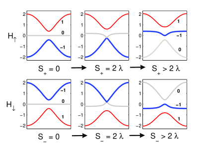
Figure 2: (Color online) The band dispersions for $H_{\uparrow}$ and $H_{\downarrow}$ along $k_{x}\in[0,\pi]$, at $k_{y}=\pi/2$ . The horizontal axis is $k_{x}$ and the vertical axis is $E/t$. We take the parameter $\lambda>0$. 0 and $\pm 1$ indicate the Chern number of each band. From the left to right, $0<S_{\pm}<2\lambda$, $S_{\pm}=2\lambda$, and $S_{\pm}>2\lambda$. $H_{\downarrow}$ with $S_{-}<0$ has the identical bands structure as $H_{\uparrow}$ with $S_{+}=-S_{-}$, but opposite Chern numbers.

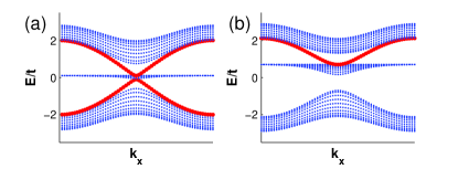
Figure 3: (Color online) Band structure of $H_{\uparrow}$ in a strip geometry. Edge state spectra are shown by dark gray lines (or red online). (a) $0<S_{+}<2\lambda$. (b) $S_{+}>2\lambda$.

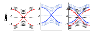
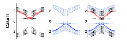
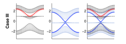
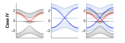
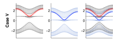
Figure 4: (Color online) Band structure in a strip geometry for five different cases. Gray large crosses and dark gray small crosses (red and blue online) represent the dispersions for the edge states. The columns from left to right are for $H_{\uparrow}^{\prime}$, $H_{\downarrow}^{\prime}$ and $H_{\uparrow}^{\prime}+H_{\downarrow}^{\prime}$, respectively. The horizontal axis is $k_{x}\in[0,\pi]$ and the vertical axis is $E/t$.

According to the Chern numbers, the edge-bulk correspondence tells that the edge states in a sample of strip geometry depend on parameters. In Fig. 3, we only present the edge state spectra of $H_{\uparrow}^{\prime}$. When $0<S_{+}<2\lambda$, the edge state spectra connect the upper and lower bands. Since the Chern number of the middle band is zero, this topologically trivial band only distorts the edge state spectra, but does not affect the existence of the edge states. The total Chern number is still 1 and the system is topologically non-trivial when the middle and lower bands are fully filled. When $S_{+}>2\lambda$, the middle band becomes topologically non-trivial, and the lower band becomes trivial. The edge state spectra only connect the middle and the upper bands.

Now we can present the evolution of edge states in the total Hamiltonian $H_{\uparrow}^{\prime}+H_{\downarrow}^{\prime}$. Five cases are listed in Fig. 4. Without loss of generality, we take $v_{s}>0$ and $v_{c}\geq 0$. In this case we have $S_{+}\geq|S_{-}|$. When time-reversal symmetry is broken, an energy gap can open between a time-reversal pair of bands. A uniform magnetism term $M\sigma_{z}$ is introduced to shift the bands of $H_{\uparrow}^{\prime}$ and $H_{\downarrow}^{\prime}$ upward and downward, respectively, without changing the Chern number of each band. A gap is opened between two middle bands. At half filling, we assume that the Fermi level is located in this gap. According to the Chern numbers and relative positions of the energy bands, the system can be categorized into five cases. Case I: $S_{+}<2|\lambda|$ and $|S_{-}|<2|\lambda|$. The total Chern numbers of three lower bands is $0$. However, the nonzero difference between the Chern numbers of $H_{\uparrow}^{\prime}$ and $H_{\downarrow}^{\prime}$ indicates QSHE. We may have two counter-propagating edge states with different spins on each edge, although these two edge states do not form a time-reversal pair as time-reversal symmetry has already been broken. Case II: $S_{+}>2|\lambda|$ and $S_{-}>2|\lambda|$. The Chern numbers of both $H_{\uparrow}^{\prime}$ and $H_{\downarrow}^{\prime}$ change to zero due to the $v_{s}$ term. When the middle band of $H_{\uparrow}^{\prime}$ is higher than the middle band of $H_{\downarrow}^{\prime}$, the system is in an insulating phase as shown in the figure. When the middle band of $H_{\uparrow}^{\prime}$ is lower, the system exhibits QSHE. Case III and Case IV: $S_{+}>2|\lambda|$ and $|S_{-}|<2|\lambda|$. Case III, when the middle band of $H_{\uparrow}^{\prime}$ is higher than the middle band of $H_{\downarrow}^{\prime}$, the total Chern number is $1$. This is a QAHE phase, in which there exists one gapless spin-up chiral edge state. Case IV: when the middle band of $H_{\uparrow}^{\prime}$ is lower than the middle band of $H_{\downarrow}^{\prime}$, the total Chern number is $0$, but it gives rise to QSHE. To distinguish Case III and Case IV, one can check the eigenvalues at $(\pi/2,\pi/2)$, and we have Case III when $v_{c}+M>2|\lambda|$. Case V: $S_{+}>2|\lambda|$ and $S_{-}<-2|\lambda|$. Due to $v_{c}$ term, the Chern numbers of both $H_{\uparrow}^{\prime}$ and $H_{\downarrow}^{\prime}$ change, and the total Chern number is $1$. Once again the system exhibits QAHE as there is only one chiral edge state.

IV FERRIMAGNETSIM AND QAHE

One of the prominent features of the model in Eq.(1) is the appearance of the flat bands due to the unequal numbers of sites of the two sublattices, even in the presence of spin-orbit coupling. These flat bands give rise to the famous flat-band ferromagnetism when the Coulomb interaction is turned on. Tasaki-92PRL ; Mielke-93CMP When the system is at half filling, the two lower bands are fully filled, and the total spin of these two bands is zero since electrons in these two bands have opposite spins. The two middle bands are degenerate. In this case, if only one single middle band is fully filled, the expectation value of the Coulomb interaction is minimized since the fully polarized electron spin in the middle band excludes the double occupancy completely at each site. In this way, the ground state of the system is ferromagnetic. The total spin is given by the degeneracy of the flat band, $S_{tot}=N\hbar/2$.Lieb-89PRL ; Shen-98IJMP Furthermore, since the antiferromagnetic correlation is dominant in the half-filled Hubbard model, this ground state is actually ferrimagnetic in which ferromagnetic and antiferromagnetic long range orders coexist.Shen-94PRL When the spin-orbit coupling is present, the flat bands will be distorted by the ferrimagnetism. When the coupling is strong, the ferrimagnetism would significantly distort the flat bands and is suppressed. Let us focus on the case of weak spin-orbit coupling, in which the band is expected to be almost flat. It is still possible that the ferrimagnetism could survive if the Coulomb interaction is strong enough over the band distortion.Tasaki-96JSP Thus the combination of the flat band and the Coulomb interaction provides a reliable mechanism to realize the spin-dependent staggered potential in this system.

The Hamiltonian with the on-site and nearest-neighbor repulsive interactions has the form

$$\mathcal{H}= \mathcal{H}_{0}+\mathcal{H}_{\textrm{SO}}+U\sum_{i}n_{i\uparrow}n_{i\downarrow}+$$ (7)

$$V\sum_{\left\langle i,j\right\rangle}(n_{i}-1)(n_{j}-1)-\mu\,(\,\sum_{i}n_{i}-3N\,),$$

where $U>0$ is the on-site Coulomb potential, $V>0$ is the nearest-neighbor repulsive potential, $n_{i\alpha}=c_{i\alpha}^{\dagger}c_{i\alpha}$ is the number operator for electron with spin $\alpha$ on site $i$, and $n_{i}=n_{i\uparrow}+n_{i\downarrow}$. The chemical potential $\mu$ determines the number of electrons in the system. $N$ here is the number of unit cells, and the number of electrons is $3N$ at half filling. In the mean field approximation, the on-site interaction is decoupled asNote-MF

$$Un_{i\uparrow}n_{i\downarrow}\approx-Um_{i}\left(c_{i}^{\dagger}\sigma_{z}c_{i}\right)+\frac{U}{2}m_{i}^{2}+\frac{U}{2}n_{i},$$ (8)

where $m_{i}\equiv\langle c_{i}^{\dagger}\sigma_{z}c_{i}\rangle$ is the magnetization on site $i$. Due to the asymmetry of the two sublattices, the magnetization on site A and B are different, saying, $m_{A}$ for the sublattice $\mathbb{A}$ and $m_{B}$ for the sublattice $\mathbb{B}$. In this way the Hubbard term is reduced to

$$\sum\limits_{i}Un_{i\uparrow}n_{i\downarrow}=-Um_{A}\sum_{i\in\mathbb{A}}\,c_{i}^{\dagger}\sigma_{z}c_{i}-Um_{B}\sum_{i\in\mathbb{B}}\,c_{i}^{\dagger}\sigma_{z}c_{i},$$ (9)

At half filling, since the antiferromagnetic correlation is dominant, $m_{A}$ and $m_{B}$ have opposite signs, based on the rigorous results for the Hubbard model.Shen-94PRL ; Shen-98IJMP This can also be illustrated from the calculation of the mean field theory.

The nearest-neighbor interaction may induce the instability of charge-density wave (CDW). In the mean field approximation, we have

$$V\sum_{\langle i,j\rangle}(n_{i}-1)(n_{j}-1)$$

$$\approx 4V\sum_{i\in A}\rho_{B}(n_{i}-1)+2V\sum_{i\in B}\rho_{A}(n_{i}-1)-4VN\rho_{A}\rho_{B},$$

where $\rho_{A}\equiv\langle n_{i}-1\rangle$ for the sublattice $\mathbb{A}$ and $\rho_{B}\equiv\langle n_{i}-1\rangle$ for the sublattice $\mathbb{B}$. The CDW order parameter $\rho$ is given by $\rho_{A}=2\rho$ and $\rho_{B}=-\rho$ due to the charge conservation.

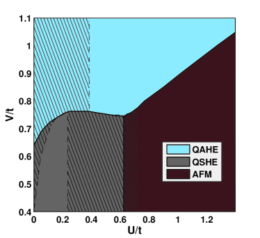
Figure 5: (Color online) $U-V$ phase diagram for $\lambda=0.1t$ at half filling. The shadow marks the gapless regions at half filling, which should be metallic with strong anomalous Hall effect and spin Hall effect.

After some tedious algebra we may have the zero-temperature mean field free energy at half filling

$$F(m_{A},m_{B},\rho,\mu)$$ (11)

$$= \;\sum_{i,\mathbf{k}}\theta\left[\mu-E_{i}(\mathbf{k})\right]\left[-\mu+E_{i}(\mathbf{k})\right]+N(E_{0}+3\mu),$$

where $\theta(x)$ is the step function, $E_{i}(\mathbf{k})$ is the eigenvalues of $H(\mathbf{k})$ in Eq. (6) with $H_{\uparrow}^{\prime}=H_{\uparrow}+(v_{s}+v_{c})\Delta+M$ and $H_{\downarrow}^{\prime}=H_{\downarrow}-(v_{s}-v_{c})\Delta-M$, where $v_{s}=U(m_{A}-m_{B})/2$, $v_{c}=4\rho V$, and $M=-U(m_{A}+m_{B})/2$. $E_{0}=Um_{A}^{2}/2+Um_{B}^{2}+8V\rho^{2}-4V\rho$. The summation runs over the whole Brillouin zone. The order parameters $m_{A}$, $m_{B}$, $\rho$, and $\mu$ can be determined self-consistently by minimizing the free energy. The variational principle

$$\frac{\delta F}{\delta m_{A}}=\frac{\delta F}{\delta m_{B}}=\frac{\delta F}{\delta\rho}=\frac{\delta F}{\delta\mu}=0$$ (12)

leads to a set of the mean field equation,

$$\sum_{i,\mathbf{\mathbf{k}}}\frac{\partial E_{i}(k)}{\partial m_{A}}\theta(\mu-E_{i}(\mathbf{k}))+NUm_{A}=0,$$

$$\sum_{i,\mathbf{k}}\frac{\partial E_{i}(\mathbf{k})}{\partial m_{B}}\theta(\mu-E_{i}(\mathbf{k}))+2NUm_{B}=0,$$

$$\sum_{i,\mathbf{k}}\frac{\partial E_{i}(\mathbf{k})}{\partial\rho}\theta(\mu-E_{i}(\mathbf{k}))+NV(16\rho-4)=0,$$

$$\sum_{i,\mathbf{k}}\theta(\mu-E_{i}(\mathbf{k}))-3N=0.$$

We solve this set of equations numerically. The calculated mean field results are consistent with the rigorous results for the Hubbard model. $m_{A}$ and $m_{B}$ have different signs, which demonstrates the existence of antiferromagnetic correlation. $m_{A}+2m_{B}\neq 0$ demonstrates the ferromagnetic correlation. If $v_{c}=0$, $m_{A}+2m_{B}=1$, which is one of the rigorous results for the Hubbard model.

Figure. 5 shows the mean field $U-V$ phase diagram for $\lambda=0.1t$ and $t>0$. The CDW order is zero when $V$ is small. $v_{s}$ and $M$ would increase with $U$ and have the same sign. The system transits from Case I to Case II through a band inversion. However we may see that the gap at half filling is not opened in the dashed area of Fig. 5. When this gap opens, Case I gives an AFM quantum spin hall effect, and Case II is an AFM insulating phase. When $V$ is large, the CDW order may become nonzero and increase with $V$. Case III can be found near the transition point where $v_{c}$ is small, and Case V can be found at larger $V$ where $v_{c}$ becomes large. They both present QAHE when the gap opens at half filling. If large $\lambda$ is chosen, the $v_{c}$ term would distort flat bands so much that the orders of $v_{s}$ and $M$ are suppressed. Thus to have a QAHE, we need strong on-site interaction $U$ and a nonzero spin-independent staggered field.

V CONCLUSIONS

We have found that the flat-band ferromagnet may exhibit QAHE after the inclusion of spin-orbit coupling on a 2D decorated lattice. The spin-orbit coupling can induce topologically non-trivial phase on this lattice, which exhibits QSHE. In the present three-band system, the existence of the topologically trivial flat band between the two non-trivial bands does not affect the formation of QSHE. The Coulomb interaction may remove the degeneracy of electrons in the flat band and lead to spontaneous symmetry breaking, which gives rise to ferrimagnetism. The coexistence of ferrimagnetism and CDW may break the balance between the helical edge states with spin up and spin down in QSHE, and make it possible that one branch of edge states is suppressed completely, and the other survives. As a result, it gives rise to QAHE.