Abstract

Remote observations of coronal holes have strongly implicated the resonant interactions of ion-cyclotron waves with ions as a principal mechanism for plasma heating and acceleration of the fast solar wind. In order to study these waves, a WKB (Wentzel-Kramers-Brillouin) linear perturbation analysis is used in the work frame of the collisionless multi-fluid model where we consider in addition to the protons a second ion component made of alpha particles. We consider a non-uniform background plasma describing a funnel region in the open coronal holes and we use the ray tracing Hamiltonian type equations to compute the ray path of the waves and the spatial variation of their properties.

1 Introduction

The ultraviolet spectroscopic observations made by SUMER (Solar Ultraviolet Measurements of Emitted Radiation) and UVCS (Ultraviolet Coronagraph Spectrometer) aboard SOHO indicated that heavy ions in the coronal holes are very hot (hotter than protons by at least their mass ratio, i.e. $T_{i}/T_{p}>m_{i}/m_{p}$) with high temperature anisotropy (see, e.g., Kohl et al., 1997; Wilhelm et al., 1998). This result is a strong indication for plasma heating through ion-cyclotron resonance (i.e., collisionless energy exchange between ions and wave fluctuations, see Stix, 1992, Chap 10) involving ion-cyclotron waves that are presumably generated in the lower corona from small-scale reconnection events (Axford and McKenzie, 1995) or locally through plasma micro-instabilities (Mecheri and Marsch, 2007; Markovskii, 2001) or turbulent cascade of low-frequency MHD-type waves towards high-frequency ion-cyclotron waves (Li et al., 1999; Hollweg, 2000; Ofman, Gary, and Viñas, 2002). This notion led to renewed interest in models involving ion heating by high-frequency ion-cyclotron waves (Isenberg, Lee, and Hollweg, 2000; Hollweg, 2000; Marsch and Tu, 2001; Vocks and Marsch, 2001; Xie, Ofman, and Viñas, 2004; Bourouaine, Vocks, and Marsch, 2008). For a detailed review on resonant ion-cyclotron interactions in the corona, see Hollweg and Isenberg (2002) and on plasma properties and physical processes in coronal holes, see Cranmer (2009). Therefore, to to allow for a good physical interpretation of the observed data, it became relevant to understand the properties of these waves in the naturally multi-ion and highly non-uniform coronal plasma, particularly in preparation to the future data which will be provided by the recently approved high resolution ESA-NASA mission ”Solar Orbiter” (planned launch in 2014).
Multi-ion linear mode analysis has been previously investigated by Mann, Hackenberg, and Marsch (1997) in the frame work of the multi-fluid model but in the simple case of a uniform background plasma. Our aim in this paper is to go beyond this previous study and consider a realistic background plasma with typical coronal profiles of density and temperature and a typical 2D open magnetic field model describing a funnel region in a coronal hole. We give a detailed study of ion-cyclotron waves by performing a Fourier plane wave analysis using the collisionless multi-fluid model where in addition to electrons (e) and protons (p), we consider a second population of ions, namely alpha particles (He²⁺, indicated by $\alpha$) with a typical coronal abundance. While neglecting the electron inertia, this model permits the consideration of ion-cyclotron wave effects that are absent from the one-fluid magnetohydrodynamics (MHD) model. Considering the WKB (Wentzel-Kramers-Brillouin) approximation, we first solve locally the dispersion relation and then perform a non-local wave analysis using the ray-tracing theory. This theory allows to compute the ray path of the waves as well as the spatial evolution of their properties while propagating through the funnel.
This paper is structured as follows. In Sect. 2, we present the background plasma configuration we use in term of density, temperature and the 2-D analytical funnel model describing open magnetic field region in a coronal hole. Then in Sect. 3, we describe how the local and non-local (ray-tracing) linear mode analysis are carried out using the multi-fluid model. The results are presented and discussed in Sect. 4, and finally our conclusions are given in Sect. 5.

2 Background plasma configuration

As a background plasma density and temperature we use the model of Fontenla, Avrett, and Loeser (1993) for the chromosphere and Gabriel (1976) for the lower corona (see Fig. 1). The 2-D potential-field model derived by Hackenberg, Marsch, and Mann (2000) is used to define the background magnetic field (Fig. 1) representing a funnel. Analytically, the two components of this model are:

$$B_{0x}(x,z) = \frac{(B_{max}-B_{00})L}{2\pi(L-d)}ln\frac{cosh\frac{2\pi z}{L}-cos(\frac{\pi d}{L}+\frac{2\pi x}{L})}{cosh\frac{2\pi z}{L}-cos(\frac{\pi d}{L}-\frac{2\pi x}{L})}$$

$$B_{0z}(x,z) = B_{00}+(B_{max}-B_{00})\left[-\frac{d}{L-d}+\frac{L}{(L-d)\pi}\right.\times$$ (1)

$$\left(arctan\frac{cosh\frac{2\pi z}{L}~{}sin\frac{\pi d}{2L}+sin(\frac{\pi d}{2L}+\frac{2\pi x}{L})}{sinh\frac{2\pi z}{L}~{}cos\frac{\pi d}{2L}}+\right.$$

$$\left.\left.arctan\frac{cosh\frac{2\pi z}{L}~{}sin\frac{\pi d}{2L}+sin(\frac{\pi d}{2L}-\frac{2\pi x}{L})}{sinh\frac{2\pi z}{L}~{}cos\frac{\pi d}{2L}}\right)\right]$$

with the following typical relevant parameters: $L=30~{}\textrm{Mm}$, $d=0.34~{}\textrm{Mm}$, $B_{00}=11.8~{}\textrm{G}$, and $B_{max}=1.5~{}\textrm{kG}$.

$\begin{array}[]{c@{\hspace{-0.1in}}c}\includegraphics[width=199.16928pt]{Mecheri-2012-fig1a.eps}\end{array}$ $\begin{array}[]{c@{\hspace{-0.1in}}c}\includegraphics[width=145.10922pt]{Mecheri-2012-fig1b.eps}\end{array}$

Figure 1: Left: Electronic density ($n_{e}$) and temperature (T) model-profiles of the chromosphere (Fontenla, Avrett, and Loeser, 1993) and the lower corona (Gabriel, 1976). Right: Funnel magnetic field geometry as obtained from a 2-D potential field model (Hackenberg, Marsch, and Mann, 2000).

3 Basic equations

The cold collisionless fluid equations for a particle species $j$ are:

$$\frac{\partial n_{j}}{\partial t}+\nabla\cdot(n_{j}\textbf{v}_{j})=0,$$ (2)

$$m_{j}n_{j}(\frac{\partial\textbf{v}_{j}}{\partial t}+\textbf{v}_{j}\cdot\nabla\textbf{v}_{j})-q_{j}n_{j}(\textbf{E}+\textbf{v}_{j}\times\textbf{B})=0,$$ (3)

where $m_{j}$, $n_{j}$, $q_{j}$ and $\textbf{v}_{j}$ are respectively the mass, density, electric charge and velocity of a species $j$. Subscript $j$ stands for electron $e$, proton $p$ or alpha particle $\alpha$ (He²⁺). The electric field E and the magnetic field B are given by Faraday’s law:

$$\nabla\times\textbf{E}=-\frac{\partial\textbf{B}}{\partial t}.$$ (4)

3.1 Linearization procedure

The linear perturbation analysis is performed by expressing all the quantities in the above equations as a sum of an unperturbed stationary part (with subscript 0) and a perturbed part (with subscript 1) much smaller than the stationary part:

$$n_{j}=n_{0j}(z)+n_{1j},\textbf{B}=\textbf{B}_{0}(x,z)+\textbf{B}_{1},\textbf{E}=\textbf{E}_{1},\textbf{v}_{j}=\textbf{v}_{1j}$$

$$\textrm{with:}~{}~{}n_{1j}\ll n_{0j},\left|\textbf{B}_{1}\right|\ll\left|\textbf{B}_{0}\right|.$$ (5)

Considering the quasi-neutrality (i.e., $\sum_{j}q_{j}n_{0j}=0$), no ambient electric field (i.e., $\textbf{E}_{0}=0$) and no background velocity (i.e., $\textbf{v}_{0j}=0$). The zero-order terms cancel out when Eq. (5) is inserted into the Eqs. (2)-(4). Neglecting the nonlinear products of the first-order terms, we get a system of coupled linear equations:

$$i\omega\frac{n_{1j}}{n_{0j}}-i\textbf{k}\cdot\textbf{v}_{1j}=0,$$ (6)

$$i\omega\textbf{v}_{1j}+\Omega_{j}\left(\frac{\textbf{E}_{1}}{\left|\textbf{B}_{0}\right|}+\textbf{v}_{1j}\times\frac{\textbf{B}_{0}}{\left|\textbf{B}_{0}\right|}\right)=\mathbf{0},$$ (7)

$$i\textbf{k}\times\textbf{E}_{1}=i\omega\textbf{B}_{1},$$ (8)

where all the perturbed quantities have been expressed in the form of a Fourier plane wave. This Fourier analysis turns all derivatives into algebraic factors, i.e. $\partial/\partial t\rightarrow-i\omega$ and $\nabla\rightarrow i\textbf{k}$, where $\omega$ is the wave frequency and k the wave vector. The quantity $\Omega_{j}=q_{j}B_{0}/m_{j}$ is the cyclotron frequency of species $j$.

3.2 Dispersion relation

To derive the dispersion relation, the above linearized equations have to be combined in order to obtain a linear relation between the current density $\textbf{J}_{1}$ and the electric field $\textbf{E}_{1}$:

$$\textbf{J}_{1}=\sigma\cdot\textbf{E}_{1},$$ (9)

where $\sigma$ is the conductivity tensor which is related to the dielectric tensor $\epsilon$ through the following relation:

$$\epsilon(\omega,\textbf{k},\textbf{r})=\textbf{I}+\frac{i}{\omega\varepsilon_{0}}\sigma(\omega,\textbf{k},\textbf{r}).$$ (10)

Finally, the local dispersion relation is obtained using the theory of electrodynamics (e.g., Stix, 1992):

$$D(\omega,\textbf{k},\textbf{r})=\textrm{Det}\left[\frac{c^{2}}{\omega^{2}}\textbf{k}\times(\textbf{k}\times\textbf{E})+\epsilon(\omega,\textbf{k},\textbf{r})\cdot\textbf{E}\right]=0,$$ (11)

where $c$ is the speed of light in vacuum and r is the large-scale position vector. We choose the wave vector k to lie in the $x-z$ plane, with $\textbf{k}=k(sin\theta,0,cos\theta)$.

3.3 Principal waves properties

In order to define certain wave properties we adopt the following coordinate system: $\textbf{e}_{B_{0}}$ and $\textbf{e}_{k}$ are the unit vectors respectively in the direction of the ambient field $\textbf{B}_{0}$ and the wave vector k (Fig. 1). We assume here that these two unit vectors lie in the $x-z$ plane. The unit vector perpendicular to $\textbf{e}_{k}$, but still in the $x-z$, is $\textbf{e}_{\phi}$. The angle between $\textbf{B}_{0}$ and k is $\phi$. In this configuration, the phase velocity $\textbf{{v}}_{ph}$ and the group velocity $\textbf{{v}}_{gr}$ are given by:

$$\textbf{v}_{\mathrm{ph}}=\frac{\omega}{k}~{}\textbf{e}_{k},~{}~{}~{}~{}~{}~{}\textbf{v}_{\mathrm{gr}}=\nabla_{\textbf{k}}\omega=\frac{\partial\omega}{\partial k}\textbf{e}_{k}+\frac{1}{k}\frac{\partial\omega}{\partial\phi}\textbf{e}_{\phi}.$$ (12)

The angle between the group velocity and the ambient field is given by:

$$\psi=\textrm{arctan}\left[\left(\frac{\partial\omega}{\partial k}sin\phi+\frac{1}{k}\frac{\partial\omega}{\partial\phi}cos\phi\right)\bigg{/}\left(\frac{\partial\omega}{\partial k}cos\phi-\frac{1}{k}\frac{\partial\omega}{\partial\phi}sin\phi\right)\right].$$ (13)

The helicity $\varrho$ (which represents the degree of circular polarization) and the electrostatic part of the wave $\xi$ are given by (Krauss-Varban, Omidi, and Quest, 1994):

$$\varrho=-2\frac{\textrm{Re}(P_{\phi})}{1+|P_{\phi}|^{2}},~{}~{}~{}~{}~{}~{}\xi=-\frac{1}{P_{\phi}}.$$ (14)

where $P_{\phi}$ represents the $\phi$-component of the polarization vector (see, e.g., Shafranov, 1967).

3.4 Ray-tracing equations

In the framework of the WKB approximation, the-ray tracing problem consists at solving a system of ordinary differential equations of the Hamiltonian form (Weinberg, 1962). These equations, which represent the equations of motion for the wave frequency $\omega$, the wave vector k, and the space coordinate r, have been formulated by Bernstein and Friedland (1984). In the simple case of a Hermitian dielectric tensor, they are given by:

$$\frac{\textrm{d}\omega}{\textrm{d}t}=-\frac{\partial D(\omega,\textbf{k},\textbf{r})/\partial t}{\partial D(\omega,\textbf{k},\textbf{r})/\partial\omega}=0,$$ (15)

$$\frac{\textrm{d}\textbf{k}}{\textrm{d}t}=~{}\frac{\partial D(\omega,\textbf{k},\textbf{r})/\partial\textbf{r}}{\partial D(\omega,\textbf{k},\textbf{r})/\partial\omega},$$ (16)

$$\frac{\textrm{d}\textbf{r}}{\textrm{d}t}=-\frac{\partial D(\omega,\textbf{k},\textbf{r})/\partial\textbf{k}}{\partial D(\omega,\textbf{k},\textbf{r})/\partial\omega}.$$ (17)

Note that Eq. (15) can be set to zero, because the dispersion relation does not explicitly depend on the time $t$ (i.e., the background plasma is stationary). The above set of differential equations represents an initial-value problem which can be solved using initial conditions obtained from the local solutions of the dispersion relation Eq. (11).

4 Numerical results

4.1 Local wave analysis

$\begin{array}[]{c@{\hspace{0.in}}c@{\hspace{0in}}c}\lx@intercol\hfil\hskip 34.14322pt\mbox{\small Two-fluid (e-p)}\hfil\lx@intercol&\lx@intercol\hfil\hskip 93.89418pt\mbox{\small Three-fluid (e-p-$\textrm{He}^{2+}$)}\hfil\lx@intercol\end{array}$

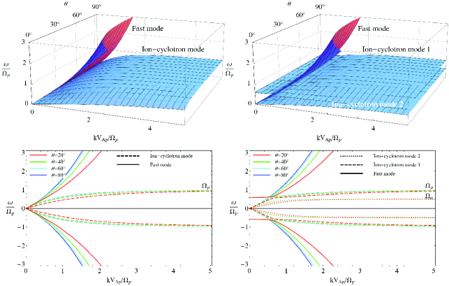
Figure 2: Top panel: Two- and three-fluid dispersion surfaces at the location (x=7.5 Mm, z=2.5 Mm) in the coronal funnel characterized by an inclination angle $\varphi\approx 79^{\circ}$ of the magnetic field with respect to the $z$-direction (see Fig. 1). Here $\omega$ and $k$ are normalized, respectively, to the proton cyclotron frequency $\Omega_{p}$ and the inertial length $\Omega_{p}/V_{Ap}$, with $V_{Ap}$ representing the proton Alfvén speed. Bottom panel: Two- and three-fluid dispersion curves at the same location and for different propagation angles $\theta$ with respect to the $z$-direction.

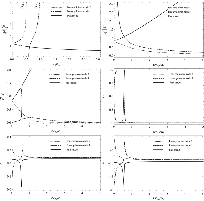
Figure 3: Basic wave properties at the location (x=7.5 Mm, z=2.5 Mm) in the coronal funnel characterized by an inclination angle $\varphi\approx 79^{\circ}$ of the magnetic field with respect to the $z$-direction (see Fig. 1). The same normalization as in Fig. (2) is used. These results are given for the case of a propagation angle $\theta=50^{\circ}$ with respect to the $z$-direction. The wave properties are : (a) refractive index $k\textrm{V}_{Ap}/\omega$, (b) phase velocity V_ph, (c) The group velocity V_gr, (d) helicity (degree of circular polarization) $\varrho$, (f) electrostatic part of the wave $\xi$, (e) angle between the direction of the group velocity and the ambient magnetic field $\psi$.

We consider a three-fluid cold plasma made of electron (e), protons (p) and alpha particles (He²⁺, indicated by $\alpha$) with a density $n_{\alpha}=0.1n_{p}$. The dispersion relation Eq.(11) is solved numerically at the funnel location (x=7.5 Mm, z=2.5 Mm) which correspond to a limit region between open and closed magnetic field lines where ion-cyclotron could potentially be generated from small scales reconnection events (Axford and McKenzie, 1995). This location is characterized by a magnetic field inclination angle of $\varphi\approx 79^{\circ}$ with respect to the normal on the solar surface. For comparison purpose, the dispersion diagrams of a two-fluid (e-p) cold plasma are also presented on Fig.(2). In this case, Eq.(11) is a quadratic polynomial of degree 4, which means that 2 modes exist and each one is represented by an oppositely propagating ($\omega>0$ and $\omega<0$) pair of waves. These modes, for which the dispersion curves and surfaces are shown on the left panels of Fig. (1), are the Ion-Cyclotron mode (IC) and the Fast mode. They are respectively the extensions of the usual Alfvén and Fast MHD modes into the high frequency domain around $\omega\approx\Omega_{p}$ where they are dispersive as compared to their non-dispersive MHD character at very low frequency ($\omega\ll\Omega_{p}$). In the case of the three-fluid model, Eq.(11) is a quadratic polynomial of degree 6. Thus, 3 modes exist which in term of phase velocity ordering are: the Ion-Cyclotron mode 1, the Ion-Cyclotron mode 2 and the Fast mode. Indeed, the results represented on the right panels of Fig.2 reveals the appearance of a second ion-cyclotron mode IC2 in addition to IC1 mode and the fast mode already present in the two-fluid model. For large k, the two IC modes reach a resonance regime at each one of the cyclotron frequencies, i.e. $\omega=\Omega_{p}$ and $\omega=\Omega_{\alpha}=\Omega_{p}/2$. The heavy ion component strongly influences the dispersion branches at small frequency $\omega/\Omega_{p}<1$ and small wave number $\textrm{kV}_{Ap}/\Omega_{p}<1$ ($\textrm{V}_{Ap}$ is the proton Alfvén speed). Indeed, we note the appearance of a Fast mode cut-off frequency approximately at $\omega_{co}/\Omega_{p}\approx 0.583$ in agreement with the algebraic relation given by Melrose (1986):

$$\omega_{co}\approx\Omega_{p}\frac{Z_{\alpha}}{A_{\alpha}}\left[\frac{1+A_{\alpha}(n_{0\alpha}/n_{0p})}{1+Z_{\alpha}(n_{0\alpha}/n_{0p})}\right],$$ (18)

with $A_{\alpha}=m_{\alpha}/m_{p}=4$ and the charge number $Z_{\alpha}=2$. Also, at k$\textrm{V}_{Ap}/\Omega_{p}\approx$0.5, the fast mode and the IC2 mode couple and convert at a frequency corresponding to the so-called cross-over frequency $\omega_{cr}/\Omega_{p}\approx 0.612$, also in conformity which the relation derived by Hollweg and Isenberg (2002):

$$\omega_{cr}\approx\Omega_{p}\left[\frac{Z_{\alpha}(n_{\alpha}/n_{p}+Z_{\alpha}/A_{\alpha}^{2})}{1+Z_{\alpha}n_{\alpha}/n_{p}}\right]^{1/2},$$ (19)

On Fig.(3), we notice that the two IC modes starts at very low frequency $\omega/\Omega_{p}\ll 1$ with a linear polarization ($\varrho=0$) in accordance with MHD theory. For increasing k, they become very rapidly circularly polarized, right handed ($\varrho=+1$) for the IC1 mode and left handed ($\varrho=-1$) for the IC2 mode. However, due to the coupling with the Fast mode, the IC1 mode transforms rapidly into a left-handed circularly-polarized mode at large k. At large k, these two modes reach a resonance regime at each one of the ion-cyclotron frequency $\omega=\Omega_{p}$ and $\omega=\Omega_{\alpha}=\Omega_{p}/2$, regime which is characterized by an infinite refractive indices $\textrm{kV}_{Ap}/\Omega_{p}$ (see Fig. 3). At very small k, the IC2 mode is characterized by a group velocity mainly parallel to the ambient field (i.e., $\psi\approx 0$) but slightly deviates from it $\mid\psi\mid\approx 8^{\circ}$ for large k (see Fig. 3). Since the direction of the group velocity indicates the flow direction of the wave energy, this means that the IC2 mode transport its energy mainly along the background magnetic field. This mode is partially electrostatic with $0.23<\xi<0.33$. On the other hand, at small k the IC1 mode is quasi-electrostatic (i.e., $\xi\approx 0$) with an energy flow fairly oblique to the magnetic field with $\mid\psi\mid\approx 20^{\circ}$ decreasing however to $\mid\psi\mid\approx 8^{\circ}$ for large k. The Fast mode starts at the cut-off frequency $\omega_{co}/\Omega_{p}=0.583$ at $\textrm{k}=0$ and is initially left-hand polarized ($\varrho=-1$). Owing to mode coupling with the IC1 mode, it rapidly changes its sense of polarization around $\textrm{kV}_{Ap}/\Omega_{p}=0.5$ to become a completely right-hand circularly-polarized wave ($\varrho=+1$). The fast mode is weakly electrostatic $\xi<0.23$ and its group velocity propagates rather obliquely to the ambient magnetic field ($10^{\circ}<\mid\psi\mid<19^{\circ}$).

4.2 Non-local wave analysis: Ray tracing

$\begin{array}[]{c@{\hspace{0.in}}c@{\hspace{0in}}c}\lx@intercol\hfil\mbox{\small Ion-Cyclotron mode 2}\hfil\lx@intercol&\lx@intercol\hfil\hskip 22.76228pt\mbox{\small Ion-Cyclotron mode 1}\hfil\lx@intercol&\lx@intercol\hfil\hskip 42.67912pt\mbox{\small Fast mode}\hfil\lx@intercol\end{array}$

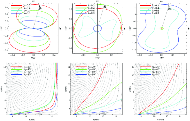
Figure 4: Top panels: Topology of the group velocity of the modes for different normalized wave number k and at the location x=7.5 Mm, z=2.5 Mm, with magnetic field $\textbf{B}_{0}$ inclination-angle $\varphi\approx 79^{\circ}$. The length of the radius at an angle of propagation $\theta$ counted from the horizontal axis ($\theta=0^{\circ}$) is equal to the group velocity. Bottom panels: The ray trajectory of the modes launched at the location (x₀=7.5 Mm, z₀=2.5 Mm) in the coronal funnel, with initial normalized wave number k₀=0.2 and at different initial angles of propagation $\theta_{0}=20^{\circ},40^{\circ},60^{\circ}~{}\textrm{and}~{}80^{\circ}$.

$\begin{array}[]{c@{\hspace{0.in}}c@{\hspace{0in}}c}\lx@intercol\hfil\mbox{\small Ion-Cyclotron mode 2}\hfil\lx@intercol&\lx@intercol\hfil\hskip 22.76228pt\mbox{\small Ion-Cyclotron mode 1}\hfil\lx@intercol&\lx@intercol\hfil\hskip 42.67912pt\mbox{\small Fast mode}\hfil\lx@intercol\end{array}$

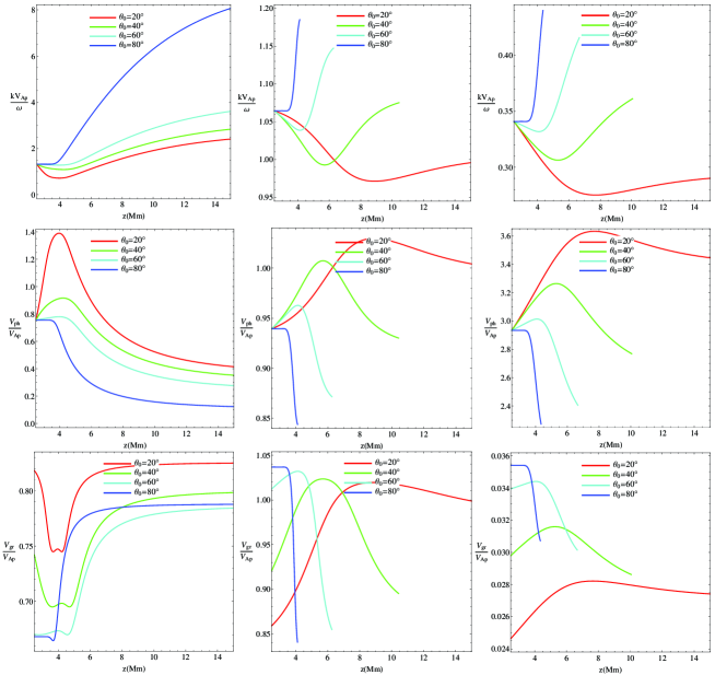
Figure 5: Variation of the basic properties of the modes as a function of height z in the solar atmosphere starting at the launch location (x₀=7.5 Mm, z₀=2.5 Mm) in the coronal funnel (with a B₀-inclination angle $\varphi_{0}\approx 79^{\circ}$) with an initial normalized wave number k₀=0.2. These results are given for different initial angles of propagation $\theta_{0}$. The wave properties are : the refractive index $k\textrm{V}_{Ap}/\omega$, the phase velocity V_ph and the group velocity V_gr.

$\begin{array}[]{c@{\hspace{0.in}}c@{\hspace{0in}}c}\lx@intercol\hfil\mbox{\small Ion-Cyclotron mode 2}\hfil\lx@intercol&\lx@intercol\hfil\hskip 22.76228pt\mbox{\small Ion-Cyclotron mode 1}\hfil\lx@intercol&\lx@intercol\hfil\hskip 42.67912pt\mbox{\small Fast mode}\hfil\lx@intercol\end{array}$

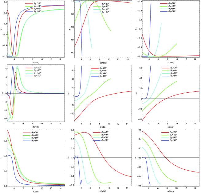
Figure 6: Variation of the basic properties of the modes as a function of height z in the solar atmosphere starting at the launch location (x₀=7.5 Mm, z₀=2.5 Mm) in the coronal funnel (with a B₀-inclination angle $\varphi_{0}\approx 79^{\circ}$) with an initial normalized wave number k₀=0.2. These results are given for different initial angles of propagation $\theta_{0}$. The wave properties are : the helicity (degree of circular polarization) $\varrho$, the angle between the direction of the group velocity and the ambient magnetic field $\psi$ and the electrostatic part of the wave $\xi$.

In this section we go beyond the local treatment of the waves and perform a non-local wave study using the ray-tracing differential equations. They are solved employing initial conditions obtained from the local solutions of the dispersion relation Eq. (11) presented in the previous section. The wave is launched at the initial location ($x_{0}=7.5$ Mm and $z_{0}=2.5$ Mm) with different initial angle of propagation, $\theta_{0}=20^{\circ},40^{\circ},60^{\circ}~{}\textrm{and}~{}80^{\circ}$. The computation have been performed for different initial values of the normalized wave number k₀, but for the sake of consistency the results will only be given for k₀=0.2. The conclusions which will be drawn are valid for all waves emitted at $\textrm{k}_{0}<1$. The ray trajectory of the waves while propagating in the funnel are shown on the bottom panels of Fig.(4) and the spatial variation of their properties as a function of the $z$-coordinate are presented on Fig.(5) and (6). On the top panels of Fig.(4) are shown the polar plots of the group velocity for the three modes corresponding to different normalized wave numbers $\textrm{kV}_{Ap}$/$\Omega_{p}$=0.2, 0.4,0.6 and 0.8. They reveal that the IC2 mode propagation is mainly anisotropic in the direction of the ambient field B₀ and cannot propagate perpendicular to it. Thus the corresponding energy mainly flows along the magnetic field lines, with maximum group velocity at parallel propagation. On the other hand, the IC1 mode and the fast mode propagate almost isotropically with no preferred direction, and consequently the energy flow is fairly isotropic.
These results are confirmed by the ray-tracing computation which clearly shows that the IC2 mode is well guided along the field lines, since the ray paths (direction of the group velocity) for various initial angle of propagation $\theta_{0}$ nicely follow the magnetic field lines (bottom panels of Fig.4). Indeed, as shown on Fig.(6), the maximal angular deviation is $\mid\psi\mid\approx 6.5^{\circ}$ at the lower part of the funnel $3<z<5\textrm{Mm}$ whereas the propagation is quasi-parallel, i.e. $\psi\approx 0^{\circ}$, in its upper part. During this quasi-parallel propagation the IC2 mode is quasi-electrostatic, i.e. $\mid\xi\mid\approx 1$, and is elliptically polarized with $0.1<\mid\varrho\mid<0.4$.
Contrary, the IC1 mode and the Fast mode are unguided modes with their ray path having mainly a strait trajectory (bottom panels of Fig.4). The angular deviation $\psi$ between the direction of the group velocity and B₀, shown on Fig.(6), varies between $-50^{\circ}$ and $70^{\circ}$ for the IC1 mode and $-40^{\circ}$ and $60^{\circ}$ for the Fast mode. The polarization is in general elliptical, right-handed ($\varrho>0$) for the IC1 mode and left-handed ($\varrho<0$) for the Fast mode, except for $\theta=20^{\circ}$ in the upper part of the funnel (z$>=6$ Mm) where it is mainly circular right-handed ($\varrho=+1$) for the IC1 mode and circular left-handed ($\varrho=-1$) for the Fast mode.

5 Conclusion

Ion-cyclotron waves propagation in a coronal funnel have been studied via a linear mode analysis using the cold three-fluid (e-p-He²⁺) model.
First local solutions of the dispersion relation have been given for a defined region in the funnel. For comparison purpose dispersion curves in the case of a two-fluid (e-p) model have been also presented. They showed the presence of two modes which are the extensions of the standard Alfvén and Fast MHD modes into the high-frequency domain ($\omega\approx\Omega_{p}$) where they are dispersive. At large wave number, the Alfvén mode (also named Ion-Cyclotron mode) experiences a resonance regime at $\omega=\Omega_{p}$. In the three-fluid model, the results have shown that the consideration of a second ion population, namely alpha particles He²⁺, strongly influences the dispersion branches as compared to the two-fluid model. Indeed, they are subject to mode coupling and conversion and show the appearance of a cut-off frequency (concerning the Fast mode). In addition to the first Ion-Cyclotron mode ”IC1” and the Fast mode previously present in the two-fluid case, we note the appearance of a second Ion-Cyclotron mode ”IC2” also subject to a resonance regime at $\omega=\Omega_{\alpha}$ at large k.
The nonlocal wave analysis, which has been performed by solving the ray tracing equations, revealed that the IC2 mode is very well guided by the magnetic field since its ray path nicely follows the field lines independently of the initial angle of propagation. This is in agreement with the topology of the IC2 mode group velocity which predicted a fairly anisotropic direction of propagation in the direction of the magnetic field with a maximum value parallel to it. As a consequence, the energy associated with this mode can carried-out to the outer corona along the open magnetic field lines. On the other hand, the IC1 mode and the Fast mode are unguided since their ray paths do not follow the magnetic field lines. They can propagate in the funnel isotropically with approximately a strait trajectory. The basic wave properties in term of phase and group velocity, polarization and other important quantities show in general a significant variation as the waves propagate in the funnel, revealing thus the importance of the non-uniformity of the medium. All these effects, and particularly the possible wave absorption and dissipation near the resonance frequencies of minor heavy ions might play a role in coronal heating.

References

- Axford and McKenzie (1995) Axford, W.I., McKenzie, J.F.: 1995, The origin of the solar wind. In: Solar Wind Eight, 31 – .
- Bernstein and Friedland (1984) Bernstein, I.B., Friedland, L.: 1984, Geometric optics in space and time varying plasmas. In: Galeev, A.A., Sudan, R.N. (eds.) Basic Plasma Physics: Handbook of Plasma Physics, Volume 1, 367.
- Bourouaine, Vocks, and Marsch (2008) Bourouaine, S., Vocks, C., Marsch, E.: 2008, Multi-Ion Kinetic Model for Coronal Loop. Astrophys. J. Lett. 680, 77 – 80. doi:10.1086/589741.
- Cranmer (2009) Cranmer, S.R.: 2009, Coronal Holes. Living Reviews in Solar Physics 6, 3.
- Fontenla, Avrett, and Loeser (1993) Fontenla, J.M., Avrett, E.H., Loeser, R.: 1993, Energy balance in the solar transition region. III - Helium emission in hydrostatic, constant-abundance models with diffusion. Astrophys. J. 406, 319 – 345. doi:10.1086/172443.
- Gabriel (1976) Gabriel, A.H.: 1976, A magnetic model of the solar transition region. Royal Society of London Philosophical Transactions Series A 281, 339 – 352. doi:10.1098/rsta.1976.0031.
- Hackenberg, Marsch, and Mann (2000) Hackenberg, P., Marsch, E., Mann, G.: 2000, On the origin of the fast solar wind in polar coronal funnels. Astron. Astrophys. 360, 1139 – 1147.
- Hollweg (2000) Hollweg, J.V.: 2000, Cyclotron resonance in coronal holes: 3. A five-beam turbulence-driven model. J. Geophys. Res. 105, 15699 – 15714. doi:10.1029/1999JA000449.
- Hollweg and Isenberg (2002) Hollweg, J.V., Isenberg, P.A.: 2002, Generation of the fast solar wind: A review with emphasis on the resonant cyclotron interaction. Journal of Geophysical Research (Space Physics) 107, 12 – 1. doi:10.1029/2001JA000270.
- Isenberg, Lee, and Hollweg (2000) Isenberg, P.A., Lee, M.A., Hollweg, J.V.: 2000, A Kinetic Model of Coronal Heating and Acceleration by Ion-Cyclotron Waves: Preliminary Results. Solar Phys. 193, 247 – 257.
- Kohl et al. (1997) Kohl, J.L., Noci, G., Antonucci, E., Tondello, G., Huber, M.C.E., Gardner, L.D., Nicolosi, P., Strachan, L., Fineschi, S., Raymond, J.C., Romoli, M., Spadaro, D., Panasyuk, A., Siegmund, O.H.W., Benna, C., Ciaravella, A., Cranmer, S.R., Giordano, S., Karovska, M., Martin, R., Michels, J., Modigliani, A., Naletto, G., Pernechele, C., Poletto, G., Smith, P.L.: 1997, First Results from the SOHO Ultraviolet Coronagraph Spectrometer. Solar Phys. 175, 613 – 644. doi:10.1023/A:1004903206467.
- Krauss-Varban, Omidi, and Quest (1994) Krauss-Varban, D., Omidi, N., Quest, K.B.: 1994, Mode properties of low-frequency waves: Kinetic theory versus Hall-MHD. J. Geophys. Res 99, 5987 – 6009.
- Li et al. (1999) Li, X., Habbal, S.R., Hollweg, J.V., Esser, R.: 1999, Heating and cooling of protons by turbulence-driven ion cyclotron waves in the fast solar wind. J. Geophys. Res. 104, 2521 – 2536. doi:10.1029/1998JA900126.
- Mann, Hackenberg, and Marsch (1997) Mann, G., Hackenberg, P., Marsch, E.: 1997, Linear mode analysis in multi-ion plasmas. Journal of Plasma Physics 58, 205 – 221.
- Markovskii (2001) Markovskii, S.A.: 2001, Generation of Ion Cyclotron Waves in Coronal Holes by a Global Resonant Magnetohydrodynamic Mode. Astrophys. J. 557, 337 – 342. doi:10.1086/321641.
- Marsch and Tu (2001) Marsch, E., Tu, C.-Y.: 2001, Heating and acceleration of coronal ions interacting with plasma waves through cyclotron and Landau resonance. J. Geophys. Res. 106, 227 – 238. doi:10.1029/2000JA000042.
- Mecheri and Marsch (2007) Mecheri, R., Marsch, E.: 2007, Coronal ion-cyclotron beam instabilities within the multi-fluid description. Astron. Astrophys. 474, 609 – 615. doi:10.1051/0004-6361:20077648.
- Melrose (1986) Melrose, D.B.: 1986, Instabilities in Space and Laboratory Plasmas, Instabilities in Space and Laboratory Plasmas, by D. B. Melrose, pp. 288. ISBN 0521305411. Cambridge, UK: Cambridge University Press, August 1986., ???.
- Ofman, Gary, and Viñas (2002) Ofman, L., Gary, S.P., Viñas, A.: 2002, Resonant heating and acceleration of ions in coronal holes driven by cyclotron resonant spectra. Journal of Geophysical Research (Space Physics) 107, 9 – 1. doi:10.1029/2002JA009432.
- Shafranov (1967) Shafranov, V.D.: 1967, Electromagnetic Waves in a Plasma. Reviews of Plasma Physics 3, 1 – 157.
- Stix (1992) Stix, T.H.: 1992, Waves in plasmas.
- Vocks and Marsch (2001) Vocks, C., Marsch, E.: 2001, A semi-kinetic model of wave-ion interaction in the solar corona. Geophys. Res. Lett. 28, 1917 – 1920. doi:10.1029/2000GL012764.
- Weinberg (1962) Weinberg, S.: 1962, Eikonal Method in Magnetohydrodynamics. Physical Review 126, 1899 – 1909. doi:10.1103/PhysRev.126.1899.
- Wilhelm et al. (1998) Wilhelm, K., Marsch, E., Dwivedi, B.N., Hassler, D.M., Lemaire, P., Gabriel, A.H., Huber, M.C.E.: 1998, The Solar Corona above Polar Coronal Holes as Seen by SUMER on SOHO. Astrophys. J. 500, 1023 – . doi:10.1086/305756.
- Xie, Ofman, and Viñas (2004) Xie, H., Ofman, L., Viñas, A.: 2004, Multiple ions resonant heating and acceleration by Alfvén/cyclotron fluctuations in the corona and the solar wind. Journal of Geophysical Research (Space Physics) 109, 8103 – . doi:10.1029/2004JA010501.