Parity breaking and scaling behavior in the spin-boson model

Abstract

We study the breaking of parity in the spin-boson model and demonstrate unique scaling behavior of the magnetization and entanglement around the critical points for the parity breaking after suppressing the infrared divergence existing inherently in the spectral functions for Ohmic and sub-Ohmic dissipations. Our treatment is basically analytical and of generality for all types of the bath. We argue that the conventionally employed spectral function is not fully reasonable and the previous justification of quantum phase transition for localization needs to be more seriously reexamined.

The spin-boson model (SBM) has been key to phenomenological descriptions of open quantum systems, in which the environment acts as a bosonic bath responsible for dissipation of the system, i.e., the spin weiss ; leggett . Besides the coherence of the spin, the correlation between the spin and the bath degrees of freedom has also attracted much attention.

The SBM hamiltonian is given by leggett

$$H=\frac{\epsilon}{2}\sigma_{z}-\frac{\Delta}{2}\sigma_{x}+\sum_{k}\omega_{k}a^{\dagger}_{k}a_{k}+\sum_{k}\lambda_{k}(a^{\dagger}_{k}+a_{k})\sigma_{z},$$ (1)

where $\sigma_{z}$ and $\sigma_{x}$ are usual Pauli operators, $\epsilon$ and $\Delta$ are, respectively, the local field (also called c-number bias leggett ) and the tunneling regarding the two levels of the spin. $a^{\dagger}_{k}$ and $a_{k}$ are creation and annihilation operators of the bath modes with frequencies $\omega_{k}$, and $\lambda_{k}$ is the coupling between the spin and the bath modes, which is governed by the spectral function $J(\omega)=\pi\sum_{k}\lambda_{k}^{2}\delta(\omega-\omega_{k})$ for $0<\omega<\omega_{c}$ with the cutoff energy $\omega_{c}$. In the infrared limit, i.e., $\omega\rightarrow$0, the power laws regarding $J(\omega)$ are of particular importance. Considering the low-energy details of the spectrum, we have $J(\omega)=2\pi\alpha\omega_{c}^{1-s}\omega^{s}$ with $0<\omega<\omega_{c}$ and the dissipation strength $\alpha$. The exponent $s$ is responsible for different bath with super-Ohmic bath $s>$1, Ohmic bath $s=$1 and sub-Ohmic bath $s<$1.

There are several approaches solving the SBM, such as the non-interacting blip approximation leggett , numerical renormalization group (NRG) vojta2 ; vojta1 ; hur ; Bu1 ; and ; rmp1 ; Bu2 ; Bu3 ; cheng , quantum Monte Carlo (QMC) winter and so on AA ; chin . The main concern in the SBM is for the localization of the spin, and quantum phase transition (QPT) between the delocalization and localization in the Ohmic dissipation has been well investigated so far hur-review . But the second-order QPT with sub-Ohmic dissipation, which is currently under intensive investigation, is not yet fully understood.

In contrast to the intensively studied QPT, we investigate the breaking of parity in the SBM. We show that variation of the parameters in Eq. (1) leads to different symmetries of the SBM hamiltonian and the parities to be broken are responsible, respectively, for localization and delocalization. The key step in our treatment is the suppression of the infrared divergence existing in the spectral functions for Ohmic and sub-Ohmic dissipations, which enables us to demonstrate unique scaling behavior of the magnetization and entanglement in the vicinity of critical points for the parity breaking. More importantly, our treatment is basically analytical and suitable for all types of the bath, by which we can fully understand the physics behind the infrared divergence and the scaling behavior.

We start from suppression of the infrared divergence in the spectral functions. With reference to the standard form of the spectral function $J(\omega)$, we introduce a distribution function $\rho(\omega)=1-e^{-P(\omega/\omega_{c})^{2}}$ with $P$ a very large number, which is a smooth variation in the function of $\omega$ with $\rho(0)=0$. So the spectral function is modified as

$$J^{\prime}(\omega)=\pi\sum_{k}\lambda_{k}^{2}\delta(\omega-\omega_{k})\rho(\omega)=2\pi\alpha\omega_{c}^{1-s}\omega^{s}\rho(\omega),$$ (2)

which fits $J(\omega)$ very well, as shown in Fig. 1 in the case of $P=10^{6}$. However, using $J^{\prime}(\omega)$, the values of integration near the zero frequency could be effectively suppressed due to the exponential factor in $\rho(\omega)$.

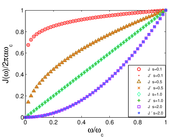
Figure 1: (color online) Comparison between $J^{\prime}(\omega)$ and $J(\omega)$ with $P=10^{6}$. $J^{\prime}(\omega)$ fits $J(\omega)$ very well with the difference hard to be distinguished from the curves.

To check how well the modified spectral function works, we compare calculations in the following with $J(\omega)$ and $J^{\prime}(\omega)$. We solve the SBM using displaced coherent states TLiu ; Zhang as the eigenfunction of Eq. (1), i.e.,

$$|\Psi\rangle=\begin{pmatrix}\sum_{\{n\}}c_{\{n\}}|\{n\}\rangle_{A}\\ \sum_{\{n\}}(-1)^{\sum_{k}n_{k}+1}d_{\{n\}}|\{n\}\rangle_{B}\end{pmatrix},$$

where $c_{\{n\}}$ and $d_{\{n\}}$ are coefficients to be determined later and $\{n\}=n_{1},\cdots,n_{N}$ are for different bosonic modes. $|\{n\}\rangle_{A(B)}$ is the product of displaced coherent states of different modes, i.e., $|\{n\}\rangle_{A(B)}=\prod_{k=1}^{N}|n_{k}\rangle_{A_{k}(B_{k})}$, where

$$|n_{k}\rangle_{A_{k}}=\frac{e^{-q_{k}^{2}/2}}{\sqrt{n_{k}!}}(a^{\dagger}_{k}+q_{k})^{n_{k}}e^{-q_{k}a_{k}^{\dagger}}|0\rangle,$$

$$|n_{k}\rangle_{B_{k}}=\frac{e^{-q_{k}^{2}/2}}{\sqrt{n_{k}!}}(a^{\dagger}_{k}-q_{k})^{n_{k}}e^{q_{k}a_{k}^{\dagger}}|0\rangle,$$

with the displacement variables $q_{k}=\lambda_{k}/\omega_{k}$ and $k=1,2,\cdots,N$. Using Schrödinger equation, we have, in the case of $\Delta\ll 1$,

$$\Big{[}\sum_{k}\omega_{k}(m_{k}-q_{k}^{2})+\frac{\epsilon}{2}\Big{]}c_{\{m\}}+\frac{\Delta}{2}d_{\{m\}}D_{\{m,m\}}=Ec_{\{m\}},$$ (3)

$$\Big{[}\sum_{k}\omega_{k}(m_{k}-q_{k}^{2})-\frac{\epsilon}{2}\Big{]}d_{\{m\}}+\frac{\Delta}{2}c_{\{m\}}D_{\{m,m\}}=Ed_{\{m\}},$$ (4)

where other terms, except $D_{\{m,m\}}$, in $D_{\{m,n\}}$ have been neglected due to the reasons in Supplementary Material SM1 . $D_{\{m,m\}}$ is given by TLiu ; Zhang

$$e^{-2\sum_{k}q_{k}^{2}}\prod_{k=1}^{N}\sum_{j=0}^{m_{k}}(-1)^{j}\frac{m_{k}!(2q_{k})^{2m_{k}-2j}}{[(m_{k}-j)!]^{2}j!}.$$

It is straightforward to yield following solutions from Eqs. (3) and (4), that is, the eigenenergies $E_{\{m\}}^{\pm}=\sum_{k}\omega_{k}(m_{k}-q_{k}^{2})\pm\sqrt{\epsilon^{2}+\Delta^{2}D^{2}_{\{m,m\}}}/2,$ and the coefficients $c^{\pm}_{\{m\}}=\mu^{\pm}_{\{m\}}/\sqrt{1+(\mu^{\pm}_{\{m\}})^{2}}$ and $d^{\pm}_{\{m\}}=1/\sqrt{1+(\mu^{\pm}_{\{m\}})^{2}}$ with $\mu^{\pm}_{\{m\}}=\Big{[}\epsilon\pm\sqrt{\epsilon^{2}+\Delta^{2}D^{2}_{\{m,m\}}}\Big{]}/\Delta D_{\{m,m\}}$. It is obvious from the expression of eigenenergies that the ground-state energy $E^{-}_{\{0\}}$ is smaller than $E^{+}_{\{0\}}$.

The above analytical treatments for Eq. (1) can be considered as complete and reliable solutions for the characteristic of the SBM SM2 . For our purpose, we may focus on the ground-state characteristic of the model to see counter-intuitive phenomena in the SBM. In such a case, the infrared divergence is reflected in the variable $D_{\{0,0\}}$, which is written as $D_{\{0,0\}}=e^{-2\sum_{k}q_{k}^{2}}$ explain0 . We first check $q_{k}^{2}$ in the case of the bath modes of the continuous spectrum vojta2 ; vojta1 . From the conventional spectral function $J(\omega)$, we have

$$\sum_{k}q_{k}^{2}=\sum_{k}\lambda_{k}^{2}/\omega^{2}_{k}=\int_{0}^{\omega_{c}}\sum_{k}\frac{\lambda_{k}^{2}}{\omega^{2}}\delta(\omega-\omega_{k})d\omega$$

$$=\int_{0}^{\omega_{c}}2\alpha\omega_{c}^{1-s}\omega^{s-2}d\omega=2\alpha\beta,~{}~{}~{}~{}~{}~{}~{}~{}~{}~{}~{}~{}~{}$$ (5)

with

$$\beta=\left\{\begin{array}[]{ll}\frac{1}{s-1}[1-(\frac{\omega_{c}}{\omega_{1}})^{1-s}]&\textrm{if $s<1$}\\ \ln(\frac{\omega_{c}}{\omega_{1}})&\textrm{if $s=1$}\\ \frac{1}{s-1}&\textrm{if $s>1$},\end{array}\right.$$

where $\alpha$ and $\omega_{c}$ are defined above in the spectral function. $\omega_{1}$ is a small quantity regarding the frequency difference from $\omega=0$. In the case of the infrared limit, i.e., $\omega_{1}\rightarrow 0$, we have $\sum_{k}q_{k}^{2}\rightarrow\infty$ if $s\leqslant 1$, which is actually caused by the uncertainty in the spectral function for $\omega_{1}\rightarrow$0. However, if using the modified spectral function $J^{\prime}(\omega)$ and repeating Eq. (5), we have $\sum_{k}q_{k}^{2}=2\alpha\beta^{\prime}$ with

$$\beta^{\prime}=\left\{\begin{array}[]{ll}\frac{1}{s-1}+\frac{1}{2P^{(s-1)/2}}[\Gamma(\frac{s-1}{2},P)-\Gamma(\frac{s-1}{2})]&\textrm{if $s\neq 1$}\\ \frac{1}{2}[\gamma+\ln(P)+\Gamma(0,P)]&\textrm{if $s=1$},\end{array}\right.$$

where $\gamma$ is the Euler-Mascheroni constant, $\Gamma(\cdot)$ is the gamma function and $\Gamma(\cdot,\cdot)$ is the upper incomplete gamma function. Since the gamma functions are finite even for a very large value of $P$, $\beta^{\prime}$ is definitely convergent. Similar results could be obtained for the bath modes of the discretized spectrum SM3 .

We have noted the results in previous publications that there are QPTs in Ohmic and sub-Ohmic dissipation cases, but not in super-Ohmic one, which exactly corresponds to the infrared divergence demonstrated above: Divergence for Ohmic and sub-Ohmic bath, but convergence for super-Ohmic bath. As a result, it is reasonable to presume that the QPT presented previously are probably induced totally or partially by the infrared divergence in the calculations using $J(\omega)$. In fact, there have been some discussions about the shortcomings in NRG methods, which cause the qualitatively incorrect results when studying quantum-critical phenomena, and spoil the determination of critical exponents and behaviors Bu2 . Additionally, there were hints that the NRG displays truncation errors or other errors in the long-range ordered phase Bu2 ; Bu3 ; Tong ; arxiv2011 .

To fully understand the characteristic of the SBM, we may first consider two special cases of Eq. (1), where we denote the case of $\epsilon\neq 0$ with $\Delta=0$ ($\epsilon=0$ with $\Delta\neq 0$) by $H(\epsilon\neq 0,\Delta\!=\!0)$ ($H(\epsilon=0,\Delta\neq 0)$). For the two special hamiltonians, we introduce, respectively, two parity operators $\Pi_{I}=\sigma_{z}$ and $\Pi_{II}=\sigma_{x}e^{i\pi\sum_{k}a^{\dagger}_{k}a_{k}}$. For $H(\epsilon\neq 0,\Delta=0)$, we have $[H(\epsilon\neq 0,\Delta=0),\Pi_{I}]=0$, with the ground state of their common eigenfunction to be $\ket{\psi_{I,0}^{-}}=\begin{pmatrix}0\\ \ket{\{0\}}_{B}\end{pmatrix}$ satisfying $\Pi_{I}\ket{\psi_{I,0}^{-}}=-\ket{\psi_{I,0}^{-}}$, i.e., an odd parity state of $\Pi_{I}$. Since $\bra{\psi_{I,0}^{-}}\sigma_{z}\ket{\psi_{I,0}^{-}}=-1$, $\ket{\psi_{I,0}^{-}}$ is always a localized state. Similarly, we have $[H(\epsilon=0,\Delta\neq 0),\Pi_{II}]=0$. The ground state of their common eigenfunction $\ket{\psi_{II,0}^{-}}=\frac{-1}{\sqrt{2}}\begin{pmatrix}\ket{\{0\}}_{A}\\ \ket{\{0\}}_{B}\end{pmatrix}$ is an even parity state of $\Pi_{II}$ with $\Pi_{II}\ket{\psi_{II,0}^{-}}=\ket{\psi_{II,0}^{-}}$. We have $\bra{\psi_{II,0}^{-}}\sigma_{z}\ket{\psi_{II,0}^{-}}=0$, meaning $\ket{\psi_{II,0}^{-}}$ to be always a delocalized state. It is evident that the odd (even) parity breaks in the variation from $\Delta=0$ with $\epsilon\neq 0$ ($\epsilon=0$ with $\Delta\neq 0$) to both $\Delta\neq 0$ and $\epsilon\neq 0$ because the hamiltonian $H$ in Eq. (1) never commutes with any of the parity operators above. This also means that the ground state of $H$ would never stay forever in delocalization or localization, but possibly moving between delocalization and localization in variation of certain characteristic parameters, such as $\alpha$. We show below the behavior of magnetization in the vicinity of critical points of the parity breaking.

The magnetization of the SBM is of importance to symbolize the transitions between delocalization and localization of the model. Using the modified spectral function and the displaced coherent states $|\{n\}\rangle_{A(B)}$, we have

$$\langle\sigma_{z}\rangle=(c^{-}_{\{0\}})^{2}-(d^{-}_{\{0\}})^{2}=\frac{-\kappa}{\sqrt{\kappa^{2}+e^{-8\alpha\beta^{\prime}}}},$$ (6)

where the average is made by the ground-state of the model and $\kappa=\epsilon/\Delta$. Since $\beta^{\prime}$ is convergent for any type of the bath, $\langle\sigma_{z}\rangle$ should be of finite value. Performing the second derivative of $\langle\sigma_{z}\rangle$ with respect to $\alpha$, we obtain a reflection point $\alpha_{c}=-\ln(2\kappa^{2})/8\beta^{\prime}$, by which Eq. (6) is rewritten as

$$\langle\sigma_{z}\rangle=\frac{-\kappa}{\sqrt{\kappa^{2}+e^{\alpha^{\prime}\ln(2\kappa^{2})}}},$$ (7)

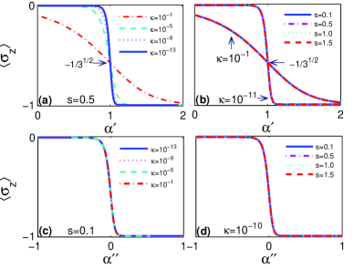
under the scaling transformation $\alpha^{\prime}=\alpha/\alpha_{c}$. For a fixed value of $\kappa$, the magnetization in Eq. (7) is only relevant to $\alpha^{\prime}$, rather than other characteristic parameters. So $\alpha_{c}$ can be regarded as a scale of the dissipation strength. In addition, if we set $\alpha^{\prime}=1$, the magnetization turns to be a constant $-1/\sqrt{3}$, which implies a fixed crossing point for different types of the bath in the magnetization with variation of $\alpha^{\prime}$ (See Fig. 2(a,b)).

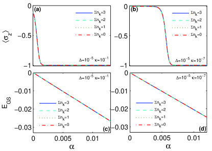
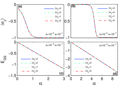
Figure 2: (color online) The scaling of the magnetization, with (a): as a function of $\alpha^{\prime}$ under sub-Ohmic dissipation for different $\kappa$; (b): as a function of $\alpha^{\prime}$ for different $\kappa$ and types of the bath; (c) and (d): as a function of $\alpha^{\prime\prime}$, which remain unchanged for the characteristic parameters $\kappa$ and $s$ in the model.

It is more interesting to demonstrate the scaling behavior of the magnetization with a displaced dissipation strength $\alpha^{\prime\prime}=(\alpha-\alpha_{c})\beta^{\prime}/\sqrt{27}$. Since $\langle\sigma_{z}(\alpha^{\prime\prime})\rangle=-1/\sqrt{1+2e^{-24\sqrt{3}\alpha^{\prime\prime}}},$ which is independent of both $\kappa$ and $s$ under the scaling transformation, the magnetization with respect to $\alpha^{\prime\prime}$, as presented in Fig. 2(c,d), remains unchanged for different types of the bath and different tunneling and localization parameters. The scaling transformation was usually used to find QPT around the critical points, where the scale invariance appears in the neighborhood of the critical points. In contrast, our results present the scale invariance in the whole region of $\alpha^{\prime\prime}$, which can be understood as the critical behavior resulting from the parity breaking regarding $\Pi_{I}$ and $\Pi_{II}$. 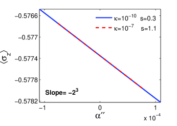It could be more clarified if we check the linear variation near the region of $\alpha^{\prime\prime}=0$ with the slope $d\langle\sigma_{z}\rangle/d\alpha^{\prime\prime}|_{\alpha^{\prime\prime}\rightarrow 0}=-8$ (See Fig. 3), which is a continuous change between the delocalization and the localization without any cusp-like behavior.

It was indicated in previous studies for the Ohmic damping at $\epsilon=0$ that quantum Kosterlitz-Thouless transition separates the delocalized phase at small $\alpha$ from the localized phase at large $\alpha$ leggett ; hur-review . In contrast, the situation of $\epsilon=0$ in our case only corresponds to delocalization and there is no possibility for any QPT. However, for Eq. (1), there is possibility of translation (with no cusp-like behavior) between the localization and delocalization in our results, where the delocalization and localization correspond, respectively, to small $\alpha$ ($\alpha<\alpha_{c}$) and large $\alpha$ ($\alpha>\alpha_{c}$). Nevertheless, our results is only relevant to the critical behavior of the parity breaking and hold for not only the sub-Ohmic damping but also other types of the bath.

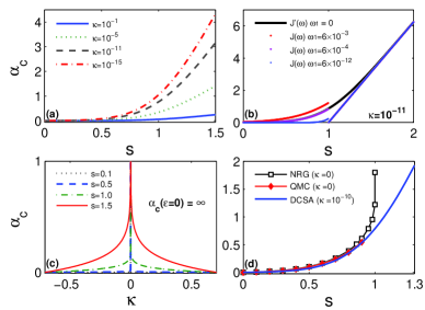
Figure 3: (color online) The magnetization in variance with $\alpha^{\prime\prime}$ in the nearby region of $\alpha^{\prime\prime}=0$ under different characteristic parameters.

Figure 4: (color online) The scale $\alpha_{c}$, where (a) as a function of $s$ under different characteristic parameters shows the smooth variance for all types of the bath; (b) as a function of $s$ compares conventional spectral function with the modified one for $\kappa=10^{-11}$; (c) in variation with $\kappa$ for different types of the bath shows the singularity at $\epsilon=0$; (d) as a function of $s$ compare our displaced coherent-state approach (DCSA) for $\kappa=10^{-10}$ with NRG and QMC for $\kappa=0$.

The scale $\alpha_{c}$ has some unique features: It is universal for different types of the bath, which means a continuous and smooth curve with respect to $s$ (See Fig. 4(a)). In contrast, if we employ the conventional spectral function, $\beta$ in the expression of $\alpha_{c}$ would yield $\alpha_{c}=0$ in the case of $s\leq$1, but finite values for $s>1$, which causes drastic changes in the variation of $\alpha_{c}$ with respect to $s$ and corresponds to the appearance of QPT around the point $s=1$ (See Fig. 4(b)). This is another evidence that the QPT for the localization in the SBM is related to the infrared divergence. On the other hand, $\epsilon=0$ is a singularity in $\alpha_{c}$, as shown in Fig. 4(c), which is, as mentioned above, due to the parity breaking regarding $\Pi_{II}$. In this sense, any characteristic parameter calculated under $\epsilon=0$ and $\epsilon\neq$0 should be very different. So the fitting in Fig. 4(d) for our approach using a negligibly small $\kappa$ with respect to the NRG and QMC at $\kappa=0$ gives the quantitative evidence that both the NRG and the QMC suffer from the infrared divergence for $s<$1 with the uncertainty equivalent to the effect of $\kappa=10^{-10}$ in the calculation without the infrared divergence.

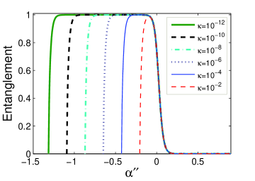
The feature of the scaling can also be reflected in entanglement. We denote the entanglement by von Neumann entropy $E=-p_{+}log_{2}p_{+}-p_{-}log_{2}p_{-}$ nc with

$$p_{\pm}=\frac{1}{2}\Big{(}1\pm\sqrt{\langle\sigma_{z}\rangle^{2}+\langle\sigma_{x}\rangle^{2}}\Big{)}=\Big{(}1\pm\sqrt{\frac{\kappa^{2}+e^{-16\alpha\beta^{\prime}}}{\kappa^{2}+e^{-8\alpha\beta^{\prime}}}}\Big{)}/2,$$ (8)

which reflects the bipartite quantum correlation between the spin and the bath. We plot in Fig. 5 the entanglement with respect to $\alpha^{\prime\prime}$ for different $\kappa$, where $\alpha\beta^{\prime}$ in Eq. (8) is replaced by $\sqrt{27}\alpha^{\prime\prime}-\ln(2\kappa^{2})/8$ under the scaling transformation. Since the magnetization reaches 0 for $\alpha<\alpha_{c}$, i.e., the delocalization, and drops to -1 if $\alpha>\alpha_{c}$, i.e., the localization (Refer to Fig. 2(c,d)), we could know from Fig. 5 that the delocalization and localization in the SBM correspond, respectively, to the increasing entanglement and the decreasing entanglement. In this sense, the scale $\alpha_{c}$ is also the reflection point for the entanglement increasing and decreasing. As a result, we may easily conclude that the ground-state of $H(\epsilon=0,\Delta\neq 0)$, which is always in delocalization, owns the entanglement increasing due to $\alpha<\alpha_{c}$ with $\alpha_{c}\rightarrow\infty$, and the ground-state of $H(\epsilon\neq 0,\Delta=0)$ is always localized with the entanglement decreasing and in most cases with disentanglement explain2 .

Figure 5: (color online) Entanglement in variance with $\alpha^{\prime\prime}$ for different $\kappa$. The curves remain unchanged for any value of $s$.

In comparison with chin ; hur ; hur-review for the relationship of the von Neumann entanglement entropy with the QPT in the SBM, no cusp-like behavior happens in our work for the entanglement changing with respect to $\alpha^{\prime\prime}$ and our results could be applied to all types of the bath. This is understandable because what we demonstrate is the scaling behavior around the critical points for the parity breaking, instead of the QPT for localization. Nevertheless, similar to the results in chin ; hur-review , we also find that the maximal entanglement appears when approaching the point $\alpha=\alpha_{c}$ from the delocalization side and then a rapid disentanglement at the localization side.

In summary, we have indicated the parity breaking in the SBM and investigated analytically the scaling behavior of the magnetization and the entanglement as well as their relationship in the neighborhood of the critical points for the parity breaking after suppressing the intrinsic infrared divergence in the spectral function. We argue that the conventionally employed spectral function is not fully reasonable and the previous conclusions drawn for the QPT happening in the Ohmic and sub-Ohmic SBM need more serious reexamination. Our analytical treatment for the scaling behavior is suitable for all types of the bath and should be of general interest, which is helpful for clarifying different numerical results in previous publications and for understanding the phenomena due to parity breaking and the physics hidden by the infrared divergence.

This work is supported by funding from WIPM, by National Fundamental Research Program of China (Grant No. 2012CB922102), and by NNSFC under Grants No. 10974225 and No. 11004226.

Supplementary Material

I Analytical solution to spin-boson model

The SBM hamiltonian is given by leggett

$$H=\frac{\epsilon}{2}\sigma_{z}-\frac{\Delta}{2}\sigma_{x}+\sum_{k}\omega_{k}a^{\dagger}_{k}a_{k}+\sum_{k}\lambda_{k}(a^{\dagger}_{k}+a_{k})\sigma_{z},$$ (9)

where $\sigma_{z}$ and $\sigma_{x}$ are usual Pauli operators, $\epsilon$ and $\Delta$ are, respectively, the local field (also called c-number bias leggett ) and tunneling regarding the two levels of the spin. $a^{\dagger}_{k}$ and $a_{k}$ are creation and annihilation operators of the bath modes with frequencies $\omega_{k}$, and $\lambda_{k}$ is the coupling between the spin and the bath modes, which is governed by the spectral function $J(\omega)=\pi\sum_{k}\lambda_{k}^{2}\delta(\omega-\omega_{k})$ for $0<\omega<\omega_{c}$ with the cutoff energy $\omega_{c}$.

We suppose the eigenfunction of Eq. (9) to be

$$|\Psi\rangle=\begin{pmatrix}\sum_{\{n\}}c_{\{n\}}|\{n\}\rangle_{A}\\ \sum_{\{n\}}(-1)^{\sum_{k}n_{k}+1}d_{\{n\}}|\{n\}\rangle_{B}\end{pmatrix},$$

where $c_{\{n\}}$ and $d_{\{n\}}$ are coefficients to be determined later and $\{n\}=n_{1},\cdots,n_{N}$ are for different Bosonic modes. $|\{n\}\rangle_{A(B)}$ is the product of displaced coherent states of different modes Zhang , i.e., $|\{n\}\rangle_{A(B)}=\prod_{k=1}^{N}|n_{k}\rangle_{A_{k}(B_{k})}$, where

$$|n_{k}\rangle_{A_{k}}=\frac{e^{-q_{k}^{2}/2}}{\sqrt{n_{k}!}}(a^{\dagger}_{k}+q_{k})^{n_{k}}e^{-q_{k}a_{k}^{\dagger}}|0\rangle,$$

$$|n_{k}\rangle_{B_{k}}=\frac{e^{-q_{k}^{2}/2}}{\sqrt{n_{k}!}}(a^{\dagger}_{k}-q_{k})^{n_{k}}e^{q_{k}a_{k}^{\dagger}}|0\rangle,$$

with the displacement variables $q_{k}=\lambda_{k}/\omega_{k}$ and $k=1,2,\cdots,N$. Using Schrödinger equation, we have

$$\Big{[}\sum_{k}\omega_{k}(m_{k}-q_{k}^{2})+\frac{\epsilon}{2}\Big{]}c_{\{m\}}+\frac{\Delta}{2}\sum_{\{n\}}d_{\{n\}}D_{\{m,n\}}=Ec_{\{m\}},$$ (10)

$$\Big{[}\sum_{k}\omega_{k}(m_{k}-q_{k}^{2})-\frac{\epsilon}{2}\Big{]}d_{\{m\}}+\frac{\Delta}{2}\sum_{\{n\}}c_{\{n\}}D_{\{m,n\}}=Ed_{\{m\}},$$ (11)

where $D_{\{m,n\}}$ is given by Zhang ; TLiu

$$e^{-2\sum_{k}q_{k}^{2}}\prod_{k=1}^{N}\sum_{j=0}^{\min[m_{k},n_{k}]}(-1)^{j}\frac{\sqrt{m_{k}!n_{k}!}(2q_{k})^{m_{k}+n_{k}-2j}}{(m_{k}-j)!(n_{k}-j)!j!}.$$

Eqs. (10) and (11) are in principle solvable, but time- and resource-consuming using currently available computing technology. For our purpose, under the condition $\Delta\ll$1, the terms of $D_{\{m,n\}}$ with $\{m\}\neq\{n\}$ play negligible roles in the equations compared to other terms with $\{m\}=\{n\}$ (The validity of the negligence of those terms is tested numerically below in Figs. 6 and 7). So Eqs. (10) and (11) can be reduced to

$$\Big{[}\sum_{k}\omega_{k}(m_{k}-q_{k}^{2})+\frac{\epsilon}{2}\Big{]}c_{\{m\}}+\frac{\Delta}{2}d_{\{m\}}D_{\{m,m\}}=Ec_{\{m\}},$$ (12)

$$\Big{[}\sum_{k}\omega_{k}(m_{k}-q_{k}^{2})-\frac{\epsilon}{2}\Big{]}d_{\{m\}}+\frac{\Delta}{2}c_{\{m\}}D_{\{m,m\}}=Ed_{\{m\}},$$ (13)

from which we may straightforwardly obtain the analytical expressions of the eigenenergies $E_{\{m\}}^{\pm}=\sum_{k}\omega_{k}(m_{k}-q_{k}^{2})\pm\sqrt{\epsilon^{2}+\Delta^{2}D^{2}_{\{m,m\}}}/2,$ and the coefficients $c^{\pm}_{\{m\}}=\mu^{\pm}_{\{m\}}/\sqrt{1+(\mu^{\pm}_{\{m\}})^{2}}$ and $d^{\pm}_{\{m\}}=1/\sqrt{1+(\mu^{\pm}_{\{m\}})^{2}}$ with $\mu^{\pm}_{\{m\}}=\Big{[}\epsilon\pm\sqrt{\epsilon^{2}+\Delta^{2}D^{2}_{\{m,m\}}}\Big{]}/\Delta D_{\{m,m\}}$.

II Validity of the truncation for the bosonic modes

In the latter half of the manuscript, we calculate the scaling behavior of the magnetization and the entanglement by only considering the ground-state of the bosonic field, i.e., $\sum n_{k}=0$. To check if this truncation works well in the case of small $\Delta$, we have calculated the magnetization with the bath modes of the discretized spectrum, based on the NRG logarithmic discretization Bu1 , where we used our modified spectral function and compared different truncations of the bosonic modes. Figs. 1 and 2 present that the magnetization remains unchanged under different truncation of the bosonic modes for different bath types, which indicate our calculation using only the ground-state of the bosonic field to be in saturation for the problem. So we may consider the results based on our analytical treatment with $\sum n_{k}=0$ to be reliable in the case of very small $\Delta$. Moreover, in the calculations for Figs. 1 and 2, we employed Eqs. (12) and (13) in the case of $\sum n_{k}=0$, and Eqs. (10) and (11) for the case of $\sum n_{k}=$1, 2 and 3. So the good fitting of the curves in the figures is also the justification of the approximation made in Eqs. (12) and (13).

Figure 6: The unchanged magnetization with respect to $\alpha$ under sub-Ohmic dissipation $s=0.2$ for different truncation of the bosonic modes, where $\Lambda=2$, $\omega_{c}=1$ and we have considered the total bosons to be 0, 1, 2 and 3, respectively.

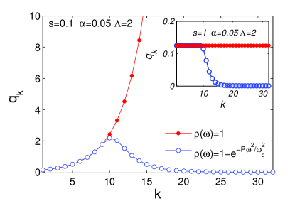
Figure 7: The unchanged magnetization with respect to $\alpha$ under super-Ohmic dissipation $s=1.2$ for different truncation of the bosonic modes, where $\Lambda=2$, $\omega_{c}=1$ and we have considered the total bosons to be 0, 1, 2 and 3, respectively.

Figure 8: (color online) $q_{k}$ as the function of $k$ under the treatment of the NRG logarithmic discretization using $J(\omega)$ (the curve with red dots) and $J^{\prime}(\omega)$ (the curve with blue circles), where $s=0.1$, $\alpha=0.05$, $P=10^{6}$, $\omega_{c}=1$ and $\Lambda=2$. The inset is for $s=1$ with the same values of $\alpha$, $P$ and $\Lambda$.

III Calculation for bath modes of the discretized spectrum

For the bath modes of the discretized spectrum, we modify the parameters in Eq. (9) by the NRG logarithmic discretization Bu1 as

$$\omega_{k}=\xi_{k}=\gamma_{k}^{-2}\int_{\Lambda^{-(k+1)}\omega_{c}}^{\Lambda^{-k}\omega_{c}}\omega J(\omega)d\omega$$

and $\lambda_{k}=\gamma_{k}/2\sqrt{\pi}$ with $\gamma_{k}^{2}=\int_{\Lambda^{-(k+1)}\omega_{c}}^{\Lambda^{-k}\omega_{c}}J(\omega)d\omega$. In such a case, it is easy to find $\sum_{k}q_{k}^{2}=\sum_{k}\gamma_{k}^{2}/(4\pi\xi_{k}^{2}),$ which, as demonstrated in Fig. 8 for $s\leq 1$, is divergent with $J(\omega)$ but convergent using $J^{\prime}(\omega)$. So our modified spectral function could effectively suppress the infrared divergence in the study of the SBM.

References

(1) U. Weiss, Quantum dissipative Systems (World
Scientific, Singapore, 1999).
(2) A. J. Leggett, S. Chakravarty, A.T. Dorsey, M.P.A. Fisher,
A. Garg, W. Zwerger, Rev. Mod. Phys. 59, 1 (1987).
(3) R. Bulla, N.-H. Tong, and M. Vojta, Phys. Rev. Lett.
91, 170601 (2003).
(4) M. Vojta, N. H. Tong and R. Bulla, Phys. Rev. Lett.
94, 070604 (2005); ibid, 102, 249904(E) (2009).
(5) R. Bulla, H.-J. Lee, N.-H. Tong, and M. Vojta, Phys. Rev. B
71, 045122 (2005).
(6) K. Le Hur, P. Doucet-Beaupre, and W. Hofstetter, Phys. Rev.
Lett. 99, 126801 (2007).
(7) F. B. Anders, R. Bulla, and M. Vojta, Phys. Rev. Lett. 98, 210402
(2007).
(8) R. Bulla, T. A. Costi, and T. Pruschkenan, Rev.
Mod. Phys. 80, 395 (2008).
(9) M. Vojta, R. Bulla, F. Güttge, and F. Anders, Phys. Rev. B
81, 075122 (2010).
(10) S. Florens, A. Freyn, D. Venturelli, and R. Narayanan, Phys. Rev.
B 84, 155110 (2011).
(11) M. Cheng, M. T. Glossop and K. Ingersent, Phys. Rev. B
80, 165113 (2009).
(12) A. Winter, H. Rieger, M. Vojta and R. Bulla, Phys. Rev.
Lett. 102, 030601 (2009).
(13) A. Alvermann and H. Fehske, Phys. Rev. Lett. 102,
150601 (2009).
(14) A. W. Chin, J. Prior, S. F. Huelga, and M. B. Plenio, Phys.
Rev. Lett. 107, 160601 (2011).
(15) K. Le Hur, Ann. Phys. 323, 2208 (2008).
(16) See section I in Supplemental Material for technical
parts of the approximation that are not essential for the
understanding of this Letter.
(17) T. Liu, K. L. Wang and M. Feng, Europhys. Lett. 86, 54003 (2009).
(18) Y. Y. Zhang, Q. H. Chen and K. L. Wang, Phys. Rev. B 81, 121105(R) (2010).
(19) See Supplementary Material for the proof.
(20) The infrared divergence also exists in other terms of with 0.
In our following analytical treatment, however, we only consider the ground-state bosonic mode, i.e., ,
which could present an identical description, in the case of small tunneling, to the situation involving excited-state
bosonic modes, as shown in Sec II in Suplementary Material.
(21) See Supplementary Material for the numerical results which are not essential for the
(22) Y.-H. Hou and N.-H. Tong, Euro. Phys. J. B 78, 127 (2010).
(23) M. Vojta, arXiv: cond-mat-stat-mech/1201.4922v1 (2011).
(24) M. A. Nielsen and I. L. Chuang, Quantum Computation and Quantum Information
(Cambridge University Press, Cambridge, England, 2004).
(25) Despite the similarity between the cases of and ,
we could not simply use the expression
for the case of ,
which yields . The correct way to
understand the situation of should return to Eqs. (3) and
(4), and we could easily obtain the trivial solution for ,
i.e., constant localization of the spin.