Computing $L_{1}$ Shortest Paths among Polygonal Obstacles in the Plane

Abstract

Given a point $s$ and a set of $h$ pairwise disjoint polygonal obstacles of totally $n$ vertices in the plane, we present a new algorithm for building an $L_{1}$ shortest path map of size $O(n)$ in $O(T)$ time and $O(n)$ space such that for any query point $t$, the length of the $L_{1}$ shortest obstacle-avoiding path from $s$ to $t$ can be reported in $O(\log n)$ time and the actual shortest path can be found in additional time proportional to the number of edges of the path, where $T$ is the time for triangulating the free space. It is currently known that $T=O(n+h\log^{1+\epsilon}h)$ for an arbitrarily small constant $\epsilon>0$. If the triangulation can be done optimally (i.e., $T=O(n+h\log h)$), then our algorithm is optimal. Previously, the best algorithm computes such an $L_{1}$ shortest path map in $O(n\log n)$ time and $O(n)$ space. Our techniques can be extended to obtain improved results for other related problems, e.g., computing the $L_{1}$ geodesic Voronoi diagram for a set of point sites in a polygonal domain, finding shortest paths with fixed orientations, finding approximate Euclidean shortest paths, etc.

1 Introduction

Computing obstacle-avoiding shortest paths in the plane is a fundamental problem in computational geometry and has many applications. The Euclidean version that measures the path length by the Euclidean distance has been well studied (e.g., see [7, 8, 15, 19, 22, 24, 25, 31, 33, 35]). In this paper, we consider the $L_{1}$ version, defined as follows. Given a point $s$ and a set of $h$ pairwise disjoint polygonal obstacles, $\mathcal{P}=\{P_{1},P_{2},\ldots,P_{h}\}$, of totally $n$ vertices in the plane, where $s$ is considered as a special point obstacle, the plane minus the interior of the obstacles is called the free space of $\mathcal{P}$. Two obstacles are pairwise disjoint if they do not intersect in their interior. The $L_{1}$ shortest path map problem, denoted by $L_{1}$-SPM, is to compute a single-source shortest path map (SPM for short) with $s$ as the source point such that for any query point $t$, an $L_{1}$ shortest obstacle-avoiding path from $s$ to $t$ can be obtained efficiently. Note that such a path can consist of any polygonal segments but the length of each segment of the path is measured by the $L_{1}$ metric.

We say that an SPM has standard query performances if for any query point $t$, the length of the $L_{1}$ shortest obstacle-avoiding path from $s$ to $t$ can be reported in $O(\log n)$ time and an actual shortest path can be found in additional time proportional to the number of edges (or turns) of the path.

If the input also includes another point $t$ and the problem only asks for one single $L_{1}$ shortest path from $s$ to $t$, then we call this problem version the $L_{1}$ shortest path problem, denoted by $L_{1}$-SP.

A closely related problem version solvable by our approach is to find shortest rectilinear paths. A rectilinear path is a path each of whose edges is parallel to a coordinate axis and its length is measured by the Euclidean distances or $L_{1}$ distances of its segments (they are the same for rectilinear paths). Rectilinear shortest paths are used widely in VLSI design and network wire-routing applications. As shown in [10, 27, 29, 30], it is easy to convert an arbitrary polygonal path to a rectilinear path with the same $L_{1}$ length. Thus, in this paper, we focus on computing polygonal paths measured by the $L_{1}$ distance.

1.1 Previous Work

The $L_{1}$-SP problem has been studied extensively (e.g., see [6, 10, 11, 27, 29, 30, 36]). In general, there are two approaches for solving this problem: Constructing a sparse “path preserving” graph (analogous to a visibility graph), and the continuous Dijkstra paradigm. Clarkson, Kapoor, and Vaidya [10] constructed a graph of $O(n\log n)$ nodes and $O(n\log n)$ edges such that a shortest path can be found in the graph in $O(n\log^{2}n)$ time; subsequently, they gave an algorithm of $O(n\log^{1.5}n)$ time and $O(n\log^{1.5}n)$ space [11]. Based on some observations, Chen, Klenk, and Tu [6] showed that the problem was solvable in $O(n\log^{1.5}n)$ time and $O(n\log n)$ space. By applying the continuous Dijkstra paradigm, Mitchell [29, 30] solved the problem in $O(n\log n)$ time and $O(n)$ space. An $O(n+h\log h)$ time lower bound can be established for solving $L_{1}$-SP (e.g., based on the results in [12]). Hence, Mitchell’s algorithm is worst-case optimal. Recently, by using a corridor structure and building a smaller path preserving graph, Inkulu and Kapoor [21] solved the $L_{1}$-SP problem in $O(n+h\log^{1.5}n)$ time and $O(n+h\log^{1.5}h)$ space.

For the query version of the problem, i.e., $L_{1}$-SPM, Mitchell’s algorithm [29, 30] builds an SPM of size $O(n)$ in $O(n\log n)$ time and $O(n)$ space with the standard query performances.

In addition, for the convex case where all polygonal obstacles in $\mathcal{P}$ are convex, to our best knowledge, we are not aware of any previous better results than those mentioned above.

1.2 Our Results

We present an algorithm for $L_{1}$-SPM that builds an SPM of size $O(n)$ in $O(T)$ time and $O(n)$ space with the standard query performances, where $T$ always refers to the time for triangulating the free space of $\mathcal{P}$ in the paper. It is obvious to see that given an SPM, we can always add $h-1$ line segments in the free space to connect the obstacles in $\mathcal{P}$ together to obtain a single simple polygon and then triangulate the free space, in totally $O(n)$ time [2, 3]. It is currently known that $T=\Omega(n+h\log h)$ and $T=O(n+h\log^{1+\epsilon}h)$ [2], where $\epsilon$ is an arbitrarily small positive constant. Therefore, we essentially solve $L_{1}$-SPM in $\Theta(T)$ time. In other words, our result shows that building an SPM is equivalent to triangulating the free space of $\mathcal{P}$ in terms of the running time.

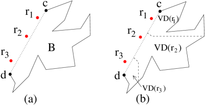
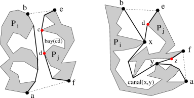
Our approach uses Mitchell’s algorithm [29, 30] as a procedure and further explores the corridor structure of $\mathcal{P}$ [25]. One interesting observation we found is that to find an $L_{1}$ shortest path among convex obstacles, it is sufficient to consider only the at most four extreme vertices (along the horizontal and vertical directions) of each obstacle (these vertices define a core for each obstacle). Mitchell’s algorithm is then applied to these cores, which takes only $O(h\log h)$ time. More work needs to be done for computing an SPM. For example, one key result we have is that we give an $O(n^{\prime}+m^{\prime})$ time algorithm for a special case of constructing the $L_{1}$ geodesic Voronoi diagram in a simple polygon of $n^{\prime}$ vertices for $m^{\prime}$ weighted point sites, where the sites all lie outside the polygon and influence the polygon through one (open) edge (see Fig. 1). We are not aware of any specific previous work on this problem, although an $O((n^{\prime}+m^{\prime})\log(n^{\prime}+m^{\prime}))$ time solution may be obtained by standard techniques. Our linear time algorithm, which is clearly optimal, may be interesting in its own right.

For the convex case where all obstacles in $\mathcal{P}$ are convex, we can find a shortest $s$-$t$ path in $O(n+h\log h)$ time and $O(n)$ space since the triangulation can be done in $O(n+h\log h)$ time (e.g., by the approaches in [2, 20]); this is optimal. A by-product of our techniques, which may be a little “surprising”, is that in $O(n+h\log h)$ time and $O(n)$ space, we can build an SPM of size $O(h)$ (instead of $O(n)$) such that the shortest path length queries are answered in $O(\log h)$ time each (instead of $O(\log n)$ time).

Figure 1: (a) Three weighted sites (in red) and a simple polygon $B$ with an open edge $\overline{cd}$. The goal is to compute the $L_{1}$ geodesic Voronoi diagram in $B$ with respect to the three sites which influence $B$ only through the edge $\overline{cd}$. (b) Illustrating a possible solution: $B$ is partitioned into three Voronoi regions $\mbox{$V\!D$}(r_{i})$ for each $r_{i}$, $1\leq i\leq 3$.

1.3 Applications

Our techniques can be extended to solve other problems.

The $L_{1}$ geodesic Voronoi diagram problem, denoted by $L_{1}$-GVD, is defined as follows. Given an obstacle set $\mathcal{P}$ and a set of $m$ point sites in the free space, compute the geodesic Voronoi diagram for the $m$ point sites under the $L_{1}$ distance metric among the obstacles in $\mathcal{P}$. Mitchell [29, 30], solves the $L_{1}$-GVD problem in $O((n+m)\log(n+m))$ time. Our approach can compute it in $O(T^{\prime}+n+(m+h)\log(m+h))$ time, where $T^{\prime}$ is the time for triangulating the free space along with the $m$ point sites. It is known that $T^{\prime}=O(n+(m+h)\log^{1+\epsilon}(m+h))$ [2] or alternatively we can obtain $T^{\prime}=O(n+h\log^{1+\epsilon}h+m\log n)$. Note that when applying our algorithm to a single simple polygon $P$ of $n$ vertices, the $L_{1}$ geodesic Voronoi diagram for $m$ point sites in $P$ can be obtained in $O(n+m\log^{1+\epsilon}m)$ or $O(n+m(\log n+\log m))$ time. In comparison, the Euclidean version of the one simple polygon case was solved in $O((n+m)\log(n+m))$ time [32].

We also give better results for the shortest path problem in “fixed orientation metrics” [29, 30, 37], for which a sought path is allowed to follow only a given set of orientations. For a number $c$ of given orientations, Mitchell’s algorithm [29, 30] finds such a shortest path in $O(cn\log n)$ time and $O(cn)$ space, and our algorithm takes $O(n+h\log^{1+\epsilon}h+c^{2}h\log ch)$ time and $O(n+c^{2}h)$ space. In addition, our approach also leads to an $O(n+h\log^{1+\epsilon}h+(1/\delta)h\log\frac{h}{\sqrt{\delta}})$ time algorithm for computing a $\delta$-optimal Euclidean shortest path among polygonal obstacles for any constant $\delta>0$. For this problem, Mitchell’s algorithm [29, 30] takes $O((\sqrt{1/\delta})n\log n)$ time, and Clarkson’s algorithm [9] runs in $O((1/\delta)n\log n)$ time.

2 An Overview of Our Approaches

In this section, we give an overview of our approaches as well as the organization of this paper. Denote by $\mathcal{F}$ the free space of $\mathcal{P}$. We begin with our algorithm for the convex case, which is a key procedure for solving the general problem.

We first discuss the $L_{1}$-SP problem. In the convex case, each obstacle in $\mathcal{P}=\{P_{1},P_{2},\ldots,P_{h}\}$ is convex. For each $P_{i}\in\mathcal{P}$, we compute its core, denoted by $core(P_{i})$, which is a simple polygon by connecting the topmost, leftmost, bottommost, and rightmost points of $P_{i}$. Let $core(\mathcal{P})$ be the set of all $h$ cores of $\mathcal{P}$. For any point $t$ in the free space $\mathcal{F}$, we show that given any shortest $s$-$t$ path avoiding all cores in $core(\mathcal{P})$, we can find in $O(n)$ time a shortest $s$-$t$ path avoiding all obstacles in $\mathcal{P}$ with the same $L_{1}$ length. Based on this observation, our algorithm has two main steps: (1) Apply Mitchell’s algorithm [29, 30] on $core(\mathcal{P})$ to compute a shortest $s$-$t$ path $\pi_{core}(s,t)$ avoiding the cores in $core(\mathcal{P})$, which takes $O(h\log h)$ time since each core in $core(\mathcal{P})$ has at most four vertices; (2) based on $\pi_{core}(s,t)$, compute a shortest $s$-$t$ path avoiding all obstacles in $\mathcal{P}$ in $O(n)$ time. This algorithm takes overall $O(n+h\log h)$ time and $O(n)$ space.

To build an SPM in $\mathcal{F}$ (with respect to the source point $s$), similarly, we first apply Mitchell’s algorithm on $core(\mathcal{P})$ to compute an SPM of $O(h)$ size in the free space with respect to all cores, which can be done in $O(n+h\log h)$ time and $O(n)$ space. Based on the above SPM, in additional $O(n)$ time, we are able to compute an SPM in $\mathcal{F}$. Our results for the convex case are given in Section 3.

For the general problem where the obstacles in $\mathcal{P}$ are not necessarily convex, based on a triangulation of the free space $\mathcal{F}$, we first compute a corridor structure [25], which consists of $O(h)$ corridors and $O(h)$ junction triangles. Each corridor possibly has a corridor path. As in [25], the corridor structure can be used to partition the plane into a set $\mathcal{P}^{\prime}$ of $O(h)$ pairwise disjoint convex polygons of totally $O(n)$ vertices such that a shortest $s$-$t$ path in $\mathcal{F}$ is a shortest $s$-$t$ path avoiding the convex polygons in $\mathcal{P}^{\prime}$ and possibly containing some corridor paths. All corridor paths are contained in the polygons of $\mathcal{P}^{\prime}$. Thus, in addition to the corridor paths, finding a shortest path is reduced to an instance of the convex case. By incorporating the corridor path information into Mitchell’s continuous Dijkstra paradigm [29, 30], our algorithm for the convex case can be modified to find a shortest path in $O(T)$ time. The above algorithm is presented in Section 4.

Sections 4.3, 5, and 6 are together devoted to compute an SPM in $\mathcal{F}$ (Section 4.3 outlines the algorithm). We use the corridor structure to partition $\mathcal{F}$ into the ocean $\mathcal{M}$, bays, and canals. While the ocean $\mathcal{M}$ may be multiply connected, every bay or canal is a simple polygon. Each bay has a single common boundary edge with $\mathcal{M}$ and each canal has two common boundary edges with $\mathcal{M}$. But two bays or two canals, or a bay and a canal do not share any boundary edge. A common boundary edge of a bay (or canal) with $\mathcal{M}$ is called a gate. Thus each bay has one gate and each canal has two gates. Further, the ocean $\mathcal{M}$ is exactly the free space with respect to the convex polygonal set $\mathcal{P}^{\prime}$. By modifying our algorithm for the convex case, we can compute an SPM in $\mathcal{M}$ in $O(T)$ time. This part is discussed in Section 4.3.

Denote by $\mbox{$S\!P\!M$}(\mathcal{M})$ the SPM in $\mathcal{M}$. To obtain an SPM in $\mathcal{F}$, we need to “expand” $\mbox{$S\!P\!M$}(\mathcal{M})$ into all bays and canals through their gates. Here, a challenging subproblem is to solve efficiently a special case of the (additively) weighted $L_{1}$ geodesic Voronoi diagram problem on a simple polygon $B$: The weighted point sites all lie outside $B$ and influence $B$ through one (open) edge (e.g., see Fig. 1). The subproblem models the procedure of expanding $\mbox{$S\!P\!M$}(\mathcal{M})$ into a bay, where the polygon $B$ is the bay, the point sites are obstacle vertices in $\mathcal{M}$, the weight of each site is the length of its shortest path to the source point $s$, and the edge of the polygon (e.g., $\overline{cd}$ in Fig. 1) is the gate of the bay. As discussed before, we give a linear time solution for this subproblem in Section 5. Note that although our presentation for solving the subproblem is long and technically complicated, the algorithm itself is simple and easy to implement; our effort is mostly for simplifying the algorithm and showing its correctness.

Expanding $\mbox{$S\!P\!M$}(\mathcal{M})$ into canals, which is discussed in Section 6, is also done in linear time by using our solution for the above subproblem as a main procedure. In summary, given $\mbox{$S\!P\!M$}(\mathcal{M})$, computing an SPM for the entire free space $\mathcal{F}$ takes additional $O(n)$ time.

We discuss a little more about the above challenging subproblem. The problem may not look “challenging” at all as it can be solved by many existing techniques. For example, one may attempt to use the continuous Dijkstra approach [29, 30] to let the “wavelet” enter into the bays/canals. However, that would lead to an $O((n^{\prime}+m^{\prime})\log(n^{\prime}+m^{\prime}))$ time solution for the subproblem since it takes logarithmic time to process each event, where $n^{\prime}$ is the number of vertices of $B$ and $m^{\prime}$ is the number of weighted sites, and consequently it would take an overall $O(n\log n)$ time for building an SPM in $\mathcal{F}$. One may also want to use a sweeping algorithm [14], which would also lead to an $O((n^{\prime}+m^{\prime})\log(n^{\prime}+m^{\prime}))$ time solution since again it takes logarithmic time to process each event. In addition, the divide-and-conquer approach [34] would also take $O((n^{\prime}+m^{\prime})\log(n^{\prime}+m^{\prime}))$ time since the merge procedure takes linear time. Our algorithm for the subproblem, which can be viewed as an incremental approach, takes $O(n^{\prime}+m^{\prime})$ time. Incremental approaches have been widely used in geometric algorithms, and normally they can result in good randomized algorithms. Incremental approaches have also been used for constructing Voronoi diagrams, which usually take quadratic time. Our result demonstrates that incremental approaches are able to yield optimal deterministic solutions for building Voronoi diagrams, and the success of it hinges on discovering many geometric properties of the problem. We should point out that our techniques for solving the challenging subproblem are quite independent of other parts of the paper.

In Section 7, we generalize our techniques to solve some related problems discussed in Section 1.3. Section 8 concludes the paper.

As in [29, 30], for simplicity of discussion, we assume that the free space $\mathcal{F}$ is connected and the point $t$ is always in $\mathcal{F}$ (thus, a feasible $s$-$t$ path always exists), and no two obstacle vertices lie on the same horizontal or vertical line. In the rest of this paper, unless otherwise stated, a shortest path always refers to an $L_{1}$ shortest path and a length is always in the $L_{1}$ metric.

3 Shortest Paths among Convex Obstacles

In this section, we give our algorithms for the convex case, which are also used for the general case in later sections. Let $\mathcal{P}^{\prime}=\{P_{1}^{\prime},P_{2}^{\prime}\ldots,P_{h}^{\prime}\}$ be a set of $h$ pairwise disjoint convex polygonal obstacles of totally $n$ vertices. With respect to the source point $s$, our algorithm builds an SPM of $O(n)$ size with standard query performances in $O(n+h\log h)$ time and $O(n)$ space.

3.1 Notation and Observations

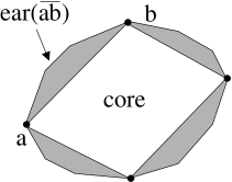
For each convex polygon $P_{i}^{\prime}\in\mathcal{P}^{\prime}$, we define its core, denoted by $core(P_{i}^{\prime})$, as the simple polygon by connecting the leftmost, topmost, rightmost, and bottommost vertices of $P_{i}^{\prime}$ with line segments (see Fig. 3). Note that $core(P_{i}^{\prime})$ is contained in $P_{i}^{\prime}$ and has at most four edges. Let $core(\mathcal{P}^{\prime})$ be the set of the cores of all obstacles in $\mathcal{P}^{\prime}$. Consider a point $t$ in the free space $\mathcal{F}$. A key observation (to be proved) is that a shortest $s$-$t$ path avoiding the cores in $core(\mathcal{P}^{\prime})$ corresponds to a shortest $s$-$t$ path avoiding the obstacles in $\mathcal{P}^{\prime}$ with the same $L_{1}$ length. Note that a path avoiding the cores in $core(\mathcal{P}^{\prime})$ may intersect the interior of some obstacles in $\mathcal{P}^{\prime}$.

To prove the above key observation, we first define some concepts. Consider an obstacle $P_{i}^{\prime}$ and $core(P_{i}^{\prime})$. For each edge $\overline{ab}$ of $core(P_{i}^{\prime})$ with vertices $a$ and $b$, if $\overline{ab}$ is not an edge of $P_{i}^{\prime}$, then it divides $P_{i}^{\prime}$ into two polygons, one of them containing $core(P_{i}^{\prime})$; we call the one that does not contain $core(P_{i}^{\prime})$ an ear of $P^{\prime}_{i}$ based on $\overline{ab}$, denoted by $ear(\overline{ab})$ (see Fig. 3). If $\overline{ab}$ is also an edge of $P_{i}$, then $ear(\overline{ab})$ is not defined. Note that $ear(\overline{ab})$ has only one edge bounding $core(P_{i}^{\prime})$, i.e., $\overline{ab}$, which we call its core edge. The other edges of $ear(\overline{ab})$ are on the boundary of $P_{i}^{\prime}$, which we call obstacle edges. There are two paths between $a$ and $b$ along the boundary of $ear(\overline{ab})$: One path is the core edge $\overline{ab}$ and the other consists of all its obstacle edges. We call the latter path the obstacle path of the ear. A line segment is positive-sloped (resp., negative-sloped) if its slope is positive (resp., negative). An ear is positive-sloped (resp., negative-sloped) if its core edge is positive-sloped (resp., negative-sloped). Note that by our assumption no two obstacle vertices lie on the same horizontal or vertical line, and thus no ear has a horizontal or vertical core edge. A point $p$ is higher (resp., lower) than another point $q$ if the $y$-coordinate of $p$ is no smaller (resp., no larger) than that of $q$. The next observation is self-evident.

Figure 2: Illustrating the core and ears of a convex obstacle; $ear(\overline{ab})$ is indicated.

Figure 3: The line segment $\overline{cd}$ penetrates $ear(\overline{ab})$; $\overline{cd}$ intersects the obstacle path of $ear(\overline{ab})$ at $e$ and $f$.

Observation 1

For any ear, its obstacle path is monotone in both the $x$- and $y$-coordinates. Specifically, consider an ear $ear(\overline{ab})$ and suppose the vertex $a$ is lower than the vertex $b$. If $ear(\overline{ab})$ is positive-sloped, then the obstacle path from $a$ to $b$ is monotonically increasing in both the $x$- and $y$-coordinates; if it is negative-sloped, then the obstacle path from $a$ to $b$ is monotonically decreasing in the $x$-coordinates and monotonically increasing in the $y$-coordinates.

For an ear $ear(\overline{ab})$ and a line segment $\overline{cd}$, we say that $\overline{cd}$ penetrates $ear(\overline{ab})$ if the following hold (see Fig. 3): (1) $\overline{cd}$ intersects the interior of $ear(\overline{ab})$, (2) neither $c$ nor $d$ is in the interior of $ear(\overline{ab})$, and (3) $\overline{cd}$ does not intersect the core edge $\overline{ab}$ at its interior. The next lemma will be useful later.

Lemma 1

Suppose a line segment $\overline{cd}$ penetrates an ear $ear(\overline{ab})$. If $\overline{cd}$ is positive-sloped (resp., negative-sloped), then $ear(\overline{ab})$ is also positive-sloped (resp., negative-sloped).

Proof: We only prove the case when $\overline{cd}$ is positive-sloped since the other case is similar.

Assume to the contrary that $ear(\overline{ab})$ is negative-sloped. Without loss of generality (WLOG), we assume $a$ is lower than $b$. By Observation 1, the obstacle path of $ear(\overline{ab})$ from $a$ to $b$ is monotonically decreasing in the $x$-coordinates. Thus, the rightmost point and leftmost point of $ear(\overline{ab})$ are $a$ and $b$, respectively. Note that $ear(\overline{ab})$ is contained in the region between the two vertical lines passing through $a$ and $b$. Since $\overline{cd}$ is positive-sloped and $\overline{ab}$ is negative-sloped, if $\overline{cd}$ intersects an interior point of $ear(\overline{ab})$, then $\overline{cd}$ must cross $\overline{ab}$ at an interior point. But since $\overline{cd}$ penetrates $ear(\overline{ab})$, $\overline{cd}$ cannot intersect any interior point of $\overline{ab}$. Hence, we have a contradiction. The lemma thus follows. $\Box$

Clearly, if $\overline{cd}$ penetrates the ear $ear(\overline{ab})$, then $\overline{cd}$ intersects the boundary of $ear(\overline{ab})$ at two points and both points lie on the obstacle path of $ear(\overline{ab})$ (e.g., see Fig. 3).

Lemma 2

Suppose a line segment $\overline{cd}$ penetrates an ear $ear(\overline{ab})$. Let $e$ and $f$ be the two points on the obstacle path of $ear(\overline{ab})$ that $\overline{cd}$ intersects. Then the $L_{1}$ length of the line segment $\overline{ef}$ is equal to that of the portion of the obstacle path of $ear(\overline{ab})$ between $e$ and $f$ (see Fig. 3).

Proof: WLOG, suppose $\overline{cd}$ is positive-sloped and $e$ is lower than $f$. By Lemma 1, $ear(\overline{ab})$ is also positive-sloped. The segment $\overline{ef}$ from $e$ to $f$ is monotonically increasing in both the $x$- and $y$-coordinates. Denote by $\widehat{ef}$ the portion of the obstacle path of $ear(\overline{ab})$ between $e$ and $f$. Since $ear(\overline{ab})$ is positive-sloped, by Observation 1, the portion $\widehat{ef}$ from $e$ to $f$ is monotonically increasing in both the $x$- and $y$-coordinates. Therefore, the $L_{1}$ lengths of $\overline{ef}$ and $\widehat{ef}$ are equal. The lemma thus follows. $\Box$

If $\overline{cd}$ penetrates $ear(\overline{ab})$, then by Lemma 2, we can obtain another path from $c$ to $d$ by replacing $\overline{ef}$ with the portion of the obstacle path of $ear(\overline{ab})$ between $e$ and $f$ such that the new path has the same $L_{1}$ length as $\overline{cd}$ and the new path does not intersect the interior of $ear(\overline{ab})$.

The results in the following lemma have been proved in [29, 30].

Lemma 3

[29, 30] There exists a shortest $s$-$t$ path in the free space such that if the path makes a turn at a point $p$, then $p$ is an obstacle vertex.

We call a shortest path that satisfies the property in Lemma 3 a vertex-preferred shortest path. Mitchell’s algorithm [29, 30] can find a vertex-preferred shortest $s$-$t$ path. Denote by $\mbox{$T\!r\!i$}(\mathcal{P}^{\prime})$ a triangulation of the free space and the space inside all obstacles. Note that the free space can be triangulated in $O(n+h\log h)$ time [2, 20] and the space inside all obstacles can be triangulated in totally $O(n)$ time [3]. Hence, $\mbox{$T\!r\!i$}(\mathcal{P}^{\prime})$ can be computed in $O(n+h\log h)$ time. The next lemma gives our key observation.

Lemma 4

Given a vertex-preferred shortest $s$-$t$ path that avoids the polygons in $core(\mathcal{P}^{\prime})$, we can find in $O(n)$ time a shortest $s$-$t$ path with the same $L_{1}$ length that avoids the obstacles in $\mathcal{P}^{\prime}$.

Proof: Consider a vertex-preferred shortest $s$-$t$ path for $core(\mathcal{P}^{\prime})$, denoted by $\pi_{core}(s,t)$. Suppose it makes turns at $p_{1},p_{2},\ldots,p_{k}$, ordered from $s$ to $t$ along the path, and each $p_{i}$ is a vertex of a core in $core(\mathcal{P}^{\prime})$. Let $p_{0}=s$ and $p_{k+1}=t$. Then for each $i=0,1,\ldots,k$, the portion of $\pi_{core}(s,t)$ from $p_{i}$ to $p_{i+1}$ is the line segment $\overline{p_{i}p_{i+1}}$, which does not intersect the interior of any core in $core(\mathcal{P}^{\prime})$. Below, we first show that we can find a path from $p_{i}$ to $p_{i+1}$ such that it avoids the obstacles in $\mathcal{P}^{\prime}$ and has the same $L_{1}$ length as $\overline{p_{i}p_{i+1}}$.

If $\overline{p_{i}p_{i+1}}$ does not intersect the interior of any obstacle in $\mathcal{P}^{\prime}$, then we are done with $\overline{p_{i}p_{i+1}}$. Otherwise, because $\overline{p_{i}p_{i+1}}$ avoids $core(\mathcal{P}^{\prime})$, it can intersects only the interior of some ears. Consider any such ear $ear(\overline{ab})$. Below, we prove that $\overline{p_{i}p_{i+1}}$ penetrates $ear(\overline{ab})$.

First, we already know that $\overline{p_{i}p_{i+1}}$ intersects the interior of $ear(\overline{ab})$. Second, it is obvious that neither $p_{i}$ nor $p_{i+1}$ is in the interior of $ear(\overline{ab})$. It remains to show that $\overline{p_{i}p_{i+1}}$ cannot intersect the core edge $\overline{ab}$ of $ear(\overline{ab})$ at the interior of $\overline{ab}$. Denote by $A^{\prime}\in\mathcal{P}^{\prime}$ the obstacle that contains $ear(\overline{ab})$. The interior of $\overline{ab}$ is in the interior of $A^{\prime}$. Since $\overline{p_{i}p_{i+1}}$ does not intersect the interior of $A^{\prime}$, $\overline{p_{i}p_{i+1}}$ cannot intersect $\overline{ab}$ at its interior. Therefore, $\overline{p_{i}p_{i+1}}$ penetrates $ear(\overline{ab})$.

Recall that we have assumed that no two obstacle vertices lie on the same horizontal or vertical line. Since both $p_{i}$ and $p_{i+1}$ are obstacle vertices, the segment $\overline{p_{i}p_{i+1}}$ is either positive-sloped or negative-sloped. WLOG, assume $\overline{p_{i}p_{i+1}}$ is positive-sloped. By Lemma 1, $ear(\overline{ab})$ is also positive-sloped. Let $e$ and $f$ denote the two intersection points between $\overline{p_{i}p_{i+1}}$ and the obstacle path of $ear(\overline{ab})$, and $\widehat{ef}$ denote the portion of the obstacle path of $ear(\overline{ab})$ between $e$ and $f$. By Lemma 2, we can replace the line segment $\overline{ef}$ ($\subseteq\overline{p_{i}p_{i+1}}$) by $\widehat{ef}$ to obtain a new path from $p_{i}$ to $p_{i+1}$ such that the new path has the same $L_{1}$ length as $\overline{p_{i}p_{i+1}}$. Further, as a portion of the obstacle path of $ear(\overline{ab})$, $\widehat{ef}$ is a boundary portion of the obstacle $A^{\prime}$ that contains $ear(\overline{ab})$, and thus $\widehat{ef}$ does not intersect the interior of any obstacle in $\mathcal{P}^{\prime}$.

By processing each ear whose interior is intersected by $\overline{p_{i}p_{i+1}}$ as above, we find a new path from $p_{i}$ to $p_{i+1}$ such that the path has the same $L_{1}$ length as $\overline{p_{i}p_{i+1}}$ and the path does not intersect the interior of any obstacle in $\mathcal{P}^{\prime}$.

By processing each segment $\overline{p_{i}p_{i+1}}$ in $\pi_{core}(s,t)$ as above for $i=0,1,\ldots,k$, we obtain another $s$-$t$ path $\pi(s,t)$ such that the $L_{1}$ length of $\pi(s,t)$ is equal to that of $\pi_{core}(s,t)$ and $\pi(s,t)$ avoids all obstacles in $\mathcal{P}^{\prime}$. Below, we show that $\pi(s,t)$ is a shortest $s$-$t$ path avoiding the obstacles in $\mathcal{P}^{\prime}$.

Since each core in $core(\mathcal{P}^{\prime})$ is contained in an obstacle in $\mathcal{P}^{\prime}$, the length of a shortest $s$-$t$ path avoiding $core(\mathcal{P}^{\prime})$ cannot be longer than that of a shortest $s$-$t$ path avoiding $\mathcal{P}^{\prime}$. Because the length of $\pi(s,t)$ is equal to that of $\pi_{core}(s,t)$ and $\pi_{core}(s,t)$ is a shortest $s$-$t$ path avoiding $core(\mathcal{P}^{\prime})$, $\pi(s,t)$ is a shortest $s$-$t$ path avoiding $\mathcal{P}^{\prime}$.

Note that the above discussion also provides a way to construct $\pi(s,t)$, which can be easily done in $O(n)$ time with the help of the triangulation $\mbox{$T\!r\!i$}(\mathcal{P}^{\prime})$. The lemma thus follows. $\Box$

Since each core in $core(\mathcal{P}^{\prime})$ is contained in an obstacle in $\mathcal{P}^{\prime}$, the corollary below follows from Lemma 4 immediately.

Corollary 1

A shortest $s$-$t$ path avoiding the obstacles in $\mathcal{P}^{\prime}$ is a shortest $s$-$t$ path avoiding the cores in $core(\mathcal{P}^{\prime})$.

3.2 Computing a Single Shortest Path

Based on Lemma 4, our algorithm for finding a single shortest $s$-$t$ path works as follows: (1) Apply Mitchell’s algorithm [29, 30] on $core(\mathcal{P}^{\prime})$ to find a vertex-preferred shortest $s$-$t$ path avoiding the cores in $core(\mathcal{P}^{\prime})$; (2) by Lemma 4, find a shortest $s$-$t$ path that avoids the obstacles in $\mathcal{P}^{\prime}$. The first step takes $O(h\log h)$ time and $O(h)$ space since the cores in $core(\mathcal{P}^{\prime})$ have totally $O(h)$ vertices. The second step takes $O(n)$ time and $O(n)$ space.

Theorem 1

Given a set of $h$ pairwise disjoint convex polygonal obstacles of totally $n$ vertices in the plane, we can find an $L_{1}$ shortest path between two points in the free space in $O(n+h\log h)$ time and $O(n)$ space.

3.3 Computing the Shortest Path Map

In this subsection, we compute the SPM for $\mathcal{P}^{\prime}$. Mitchell’s algorithm [29, 30] can compute an $O(n)$ size SPM with the standard query performances in $O(n\log n)$ time and $O(n)$ space.

By applying Mitchell’s algorithm [29, 30] on the core set $core(\mathcal{P}^{\prime})$, we can compute an $O(h)$ size SPM in $O(h\log h)$ time and $O(h)$ space, denoted by $\mbox{$S\!P\!M$}(core(\mathcal{P}^{\prime}),s)$. With a planar point location data structure [13, 26], for any query point $t$ in the free space $\mathcal{F}$, the length of a shortest $s$-$t$ path avoiding $core(\mathcal{P}^{\prime})$ can be reported in $O(\log h)$ time, which is also the length of a shortest $s$-$t$ path avoiding $\mathcal{P}^{\prime}$ by Lemma 4. We thus have the following result.

Theorem 2

Given a set of $h$ pairwise disjoint convex polygonal obstacles of totally $n$ vertices in the plane, in $O(n+h\log h)$ time and $O(n)$ space, we can construct a shortest path map of size $O(h)$ with respect to a source point $s$, such that the length of an $L_{1}$ shortest path between $s$ and any query point in the free space can be reported in $O(\log h)$ time.

The result in Theorem 2 is superior to Mitchell’s algorithm [29, 30] in three aspects, i.e., the preprocessing time, the SPM size, and the length query time. However, with the SPM for Theorem 2, an actual shortest path avoiding $\mathcal{P}^{\prime}$ between $s$ and a query point $t$ cannot be reported in additional time proportional to the number of turns of the path, although we can use this SPM to report an actual shortest path $\pi_{core}(s,t)$ between $s$ and $t$ avoiding $core(\mathcal{P}^{\prime})$ in additional time proportional to the number of turns of $\pi_{core}(s,t)$ and then find an actual shortest path avoiding $\mathcal{P}^{\prime}$ between $s$ and $t$ in another $O(n)$ time using $\pi_{core}(s,t)$ by Lemma 4.

To process queries on actual shortest paths avoiding $\mathcal{P}^{\prime}$ efficiently, in Lemma 5 below, using $\mbox{$S\!P\!M$}(core(\mathcal{P}^{\prime}),s)$, we compute an SPM for $\mathcal{P}^{\prime}$, denoted by $\mbox{$S\!P\!M$}(\mathcal{M})$, of $O(n)$ size, which has the standard query performances, i.e., answers a shortest path length query in $O(\log n)$ time and reports an actual path in additional time proportional to the number of turns of the path.

Lemma 5

Given the shortest path map $\mbox{$S\!P\!M$}(core(\mathcal{P}^{\prime}),s)$ for the core set $core(\mathcal{P}^{\prime})$, we can compute a shortest path map $\mbox{$S\!P\!M$}(\mathcal{M})$ for the obstacle set $\mathcal{P}^{\prime}$ in $O(n)$ time (with the help of the triangulation $\mbox{$T\!r\!i$}(\mathcal{P}^{\prime})$).

Proof: Note that the polygons in $\mathcal{P}^{\prime}$ are pairwise disjoint in their interior. For simplicity of discussion in this proof, we assume that any two different polygons in $\mathcal{P}^{\prime}$ have disjoint interior as well as disjoint boundaries.

Consider a cell $C_{core}(r)$ with the root $r$ in $\mbox{$S\!P\!M$}(core(\mathcal{P}^{\prime}),s)$. Recall that $r$ is always a vertex of a core in $core(\mathcal{P}^{\prime})$ and all points in $C_{core}(r)$ are visible to $r$ with respect to $core(\mathcal{P}^{\prime})$ [29, 30]. In other words, for any point $p$ in the cell $C_{core}(r)$, the line segment $\overline{rp}$ is contained in $C_{core}(r)$, and further, there exists a shortest $s$-$p$ path avoiding $core(\mathcal{P}^{\prime})$ that contains $\overline{rp}$.

Denote by $\mathcal{F}(\mathcal{P}^{\prime})$ (resp., $\mathcal{F}(core(\mathcal{P}^{\prime}))$) the free space with respect to $\mathcal{P}^{\prime}$ (resp., $core(\mathcal{P}^{\prime})$). Note that the cell $C_{core}(r)$ is a simple polygon in $\mathcal{F}(core(\mathcal{P}^{\prime}))$. We assume that $C_{core}(r)$ contains some points in $\mathcal{F}(\mathcal{P}^{\prime})$ since otherwise we do not need to consider $C_{core}(r)$.

The cell $C_{core}(r)$ may intersect some ears. In other words, certain space in $C_{core}(r)$ may be occupied by some ears. Let $C(r)$ be the subregion of $C_{core}(r)$ by removing from $C_{core}(r)$ the space occupied by all ears except their obstacle paths. Thus $C(r)$ lies in $\mathcal{F}(\mathcal{P}^{\prime})$. However, for each point $p\in C(r)$, $p$ may not be visible to $r$ with respect to $\mathcal{P}^{\prime}$. Our task here is to further decompose $C(r)$ into a set of SPM regions such that each such region has a root visible to all points in the region with respect to $\mathcal{P}^{\prime}$; further, we need to make sure that each point $q$ in an SPM region has a shortest path in $\mathcal{F}(\mathcal{P}^{\prime})$ from $s$ that contains the line segment connecting $q$ and the root of the region. For this, we first show that $C(r)$ is a connected region.

To show that $C(r)$ is connected, it suffices to show that for any point $p\in C(r)$, there is a path in $C(r)$ that connects $r$ and $p$. Consider an arbitrary point $p\in C(r)$. Since $p\in C_{core}(r)$, $\overline{rp}$ is in $C_{core}(r)$ and there is a shortest path in $\mathcal{F}(core(\mathcal{P}^{\prime}))$ from $s$ to $p$ that contains $\overline{rp}$. If the segment $\overline{rp}$ does not intersect the interior of any ear, then we are done since $\overline{rp}$ is in $C(r)$. If $\overline{rp}$ intersects the interior of some ears, then let $ear(\overline{ab})$ be one of such ears. By the proof of Lemma 4, $\overline{rp}$ penetrates $ear(\overline{ab})$. Let $e$ and $f$ be the two points on the obstacle path of $ear(\overline{ab})$ that $\overline{rp}$ intersects, and $\widehat{ef}$ be the portion of the obstacle path between $e$ and $f$. Note that if $\overline{rp}$ is horizontal or vertical, then it cannot penetrate $ear(\overline{ab})$ due to the monotonicity of its obstacle path by Observation 1. WLOG, assume $\overline{rp}$ is positive-sloped. Then by Lemma 2, $ear(\overline{ab})$ is also positive-sloped. Recall that $e$ and $f$ lie on $\overline{rp}$. WLOG, assume $r$ is higher than $p$ and $f$ is higher than $e$. Then the segment $\overline{ef}$ from $e$ to $f$ is monotonically increasing in both the $x$- and $y$-coordinates. By Observation 1, the obstacle path portion $\widehat{ef}$ from $e$ to $f$ is also monotonically increasing in both the $x$- and $y$-coordinates. As in the proof of Lemma 4, for any point $q\in\widehat{ef}$, there is a shortest path in $\mathcal{F}(core(\mathcal{P}^{\prime}))$ from $s$ to $q$ that contains $\overline{rf}$ and the portion of $\widehat{ef}$ between $f$ and $q$. Since $\overline{ef}$ is on $\overline{rp}$ contained in the cell $C_{core}(r)$, by the properties of the shortest path map $\mbox{$S\!P\!M$}(\mathcal{M})$ [29, 30], $\widehat{ef}$ is also contained in the cell $C_{core}(r)$. Thus, $\widehat{ef}$ is also contained in $C(r)$. If we process each ear whose interior intersects $\overline{rp}$ as above, we find a path in $C(r)$ that connects $r$ and $p$; further, this path has the same $L_{1}$ length as $\overline{rp}$. Hence, $C(r)$ is a connected region.

Next, we claim that for any point $p\in C(r)$, there is a shortest path in $\mathcal{F}(\mathcal{P}^{\prime})$ from $s$ to $p$ that contains $r$. Indeed, since $p\in C_{core}(r)$, there is a shortest path in $\mathcal{F}(core(\mathcal{P}^{\prime}))$ from $s$ to $p$ that contains $\overline{rp}$; let $\pi_{core}(s,r)$ be the portion of this path between $s$ and $r$. On one hand, we have shown above that there is a path from $r$ to $p$ in $C(r)$ with the same $L_{1}$ length as $\overline{rp}$. On the other hand, by Lemma 4, there exists a path in $\mathcal{F}(\mathcal{P}^{\prime})$ from $s$ to $r$ with the same length as $\pi_{core}(s,r)$. Hence, a concatenation of these two paths results in a shortest path from $s$ to $p$ in $\mathcal{F}(\mathcal{P}^{\prime})$ that contains $r$. Our claim thus follows.

The above claim and its proof also imply that decomposing $C(r)$ into a set of SPM regions is equivalent to computing an SPM in $C(r)$ with the vertex $r$ as the source point, which we denote by $\mbox{$S\!P\!M$}(C(r))$. Since $C(r)$ is a connected region and $C_{core}(r)$ is a simple polygon, we claim that $C(r)$ is a (possibly degenerate) simple polygon. This is because for any ear $E$ that intersects $C_{core}(r)$, the portion $E\cap C_{core}(r)$ lies on the boundary of the simple polygon $C_{core}(r)$; thus, removing $E$ except its obstacle path from $C_{core}(r)$ (to form $C(r)$) changes only the boundary shape of $C_{core}(r)$ but does not change the nature of a simple polygonal region (from $C_{core}(r)$ to $C(r)$). Based on the fact that $C(r)$ is a (possibly degenerate) simple polygon, $\mbox{$S\!P\!M$}(C(r))$ can be easily computed in linear time in terms of the number of edges of $C(r)$. For example, since the Euclidean shortest path between any two points in a simple polygon is also an $L_{1}$ shortest path between the two points [17], an SPM in a simple polygon with respect to the Euclidean distance is also one with respect to the $L_{1}$ distance. Therefore, we can use a corresponding shortest path algorithm for the Euclidean case (e.g., [16]) to compute each $\mbox{$S\!P\!M$}(C(r))$ in our problem.

Note that our discussion above also implies that given $\mbox{$S\!P\!M$}(core(\mathcal{P}^{\prime}),s)$, for each cell $C_{core}(r)$ with a root $r$, we can compute the corresponding $\mbox{$S\!P\!M$}(C(r))$ separately. Clearly, the $\mbox{$S\!P\!M$}(C(r))$’s corresponding to all cells in $\mbox{$S\!P\!M$}(core(\mathcal{P}^{\prime}),s)$ constitute a shortest path map $\mbox{$S\!P\!M$}(\mathcal{M})$ for $\mathcal{P}^{\prime}$.

Due to the planarity of the cell regions involved, the total number of edges of all $C(r)$’s is $O(n)$. Given a triangulation $\mbox{$T\!r\!i$}(\mathcal{P}^{\prime})$, all regions $C(r)$ can be obtained in totally $O(n)$ time. Computing all $\mbox{$S\!P\!M$}(C(r))$’s also takes totally $O(n)$ time. Thus, $\mbox{$S\!P\!M$}(\mathcal{M})$ can be constructed in $O(n)$ time. The lemma thus follows. $\Box$

Theorem 2 and Lemma 5 together lead to the following result.

Theorem 3

Given a set of $h$ pairwise disjoint convex polygonal obstacles of totally $n$ vertices in the plane, in $O(n+h\log h)$ time and $O(n)$ space, we can construct a shortest path map of size $O(n)$ with respect to a source point $s$, such that given any query point $t$ in the free space, the length of an $L_{1}$ shortest $s$-$t$ path can be reported in $O(\log h)$ time and an actual path can be found in $O(\log n+k)$ time where $k$ is the number of turns of the path.

4 Shortest Paths among General Polygonal Obstacles

In this section, we consider the general case, i.e., the obstacles in $\mathcal{P}$ are not necessarily convex. In the following, in Section 4.1, we review the corridor structure [25], and introduce the ocean $\mathcal{M}$. In Section 4.2, we present the algorithm for computing a single shortest path and the similar idea also computes an SPM for $\mathcal{M}$, i.e., $\mbox{$S\!P\!M$}(\mathcal{M})$. In Section 4.3, we outline our algorithm for computing an SPM in the entire free space $\mathcal{F}$.

4.1 Preliminaries

For simplicity of discussion, we assume that all obstacles are contained in a large rectangle $\mathcal{R}$ (see Fig. 5). Let $\mathcal{F}$ be the free space inside $\mathcal{R}$. Let $t$ be an arbitrary point in $\mathcal{F}$.

Figure 4: Illustrating a triangulation of the free space among two obstacles and the corridors (with red solid curves). There are two junction triangles indicated by the large dots inside them, connected by three solid (red) curves. Removing the two junction triangles results in three corridors.

Figure 5: Illustrating an open hourglass (left) and a closed hourglass (right) with a corridor path linking the apices $x$ and $y$ of the two funnels. The dashed segments are diagonals. The paths $\pi(a,b)$ and $\pi(e,f)$ are shown with thick solid curves.

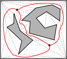
We first review the corridor structure [25]. Denote by $\mbox{$T\!r\!i$}(\mathcal{F})$ a triangulation of $\mathcal{F}$. Let $G(\mathcal{F})$ denote the (planar) dual graph of $\mbox{$T\!r\!i$}(\mathcal{F})$, i.e., each node of $G(\mathcal{F})$ corresponds to a triangle in $\mbox{$T\!r\!i$}(\mathcal{F})$ and each edge connects two nodes of $G(\mathcal{F})$ corresponding to two triangles sharing a diagonal of $\mbox{$T\!r\!i$}(\mathcal{F})$. The degree of each node in $G(\mathcal{F})$ is at most three. As in [25], at least one node dual to a triangle incident to each of $s$ and $t$ is of degree three. Based on $G(\mathcal{F})$, we compute a planar 3-regular graph, denoted by $G^{3}$ (the degree of each node in $G^{3}$ is three), possibly with loops and multi-edges, as follows. First, we remove every degree-one node from $G(\mathcal{F})$ along with its incident edge; repeat this process until no degree-one node exists. Second, remove every degree-two node from $G(\mathcal{F})$ and replace its two incident edges by a single edge; repeat this process until no degree-two node exists. The resulting graph is $G^{3}$ (e.g., see Fig. 5). The resulting graph $G^{3}$ has $O(h)$ faces, $O(h)$ nodes, and $O(h)$ edges [25]. Each node of $G^{3}$ corresponds to a triangle in $\mbox{$T\!r\!i$}(\mathcal{F})$, which is called a junction triangle (e.g., see Fig. 5). The removal of all junction triangles from $G^{3}$ results in $O(h)$ corridors, each of which corresponds to one edge of $G^{3}$.

The boundary of a corridor $C$ consists of four parts (see Fig. 5): (1) A boundary portion of an obstacle $P_{i}\in\mathcal{P}$, from a point $a$ to a point $b$; (2) a diagonal of a junction triangle from $b$ to a boundary point $e$ on an obstacle $P_{j}\in\mathcal{P}$ ($P_{i}=P_{j}$ is possible); (3) a boundary portion of the obstacle $P_{j}$ from $e$ to a point $f$; (4) a diagonal of a junction triangle from $f$ to $a$. The two diagonals $\overline{be}$ and $\overline{af}$ are called the doors of $C$. The corridor $C$ is a simple polygon. Let $\pi(a,b)$ (resp., $\pi(e,f)$) denote the shortest path from $a$ to $b$ (resp., $e$ to $f$) inside $C$. The region $H_{C}$ bounded by $\pi(a,b),\pi(e,f)$, and the two diagonals $\overline{be}$ and $\overline{fa}$ is called an hourglass, which is open if $\pi(a,b)\cap\pi(e,f)=\emptyset$ and closed otherwise (see Fig. 5). If $H_{C}$ is open, then both $\pi(a,b)$ and $\pi(e,f)$ are convex chains and are called the sides of $H_{C}$; otherwise, $H_{C}$ consists of two “funnels” and a path $\pi_{C}=\pi(a,b)\cap\pi(e,f)$ joining the two apices of the two funnels, called the corridor path of $C$. The two funnel apices connected by the corridor path are called the corridor path terminals. Each funnel side is also convex. We compute the hourglass for each corridor. After the triangulation, computing the hourglasses for all corridors takes totally $O(n)$ time.

Let $Q$ be the union of all junction triangles and hourglasses. Then $Q$ consists of $O(h)$ junction triangles, open hourglasses, funnels, and corridor paths. As shown in [21], there exists a shortest $s$-$t$ path $\pi(s,t)$ avoiding the obstacles in $\mathcal{P}$ which is contained in $Q$. Consider a corridor $C$. If $\pi(s,t)$ contains an interior point of $C$, then the path $\pi(s,t)$ must intersect both doors of $C$; further, if the hourglass $H_{C}$ of $C$ is closed, then we claim that we can make the corridor path of $C$ entirely contained in $\pi(s,t)$. Suppose $\pi(s,t)$ intersects the two doors of $C$, say, at two points $p$ and $q$ respectively. Then since $C$ is a simple polygon, a Euclidean shortest path between $p$ and $q$ inside $C$, denoted by $\pi_{E}(p,q)$, is also an $L_{1}$ shortest path in $C$ [17]. Note that $\pi_{E}(p,q)$ must contain the corridor path of $C$. If we replace the portion of $\pi(s,t)$ between $p$ and $q$ by $\pi_{E}(p,q)$, then we obtain a new $L_{1}$ shortest $s$-$t$ path that contains the corridor path $\pi_{C}$. For simplicity, we still use $\pi(s,t)$ to denote the new path. In other words, $\pi(s,t)$ has the property that if $\pi(s,t)$ intersects both doors of $C$ and the hourglass $H_{C}$ is closed, then the corridor path of $C$ is contained in $\pi(s,t)$.

Let $\mathcal{M}$ be $Q$ minus the corridor paths. We call $\mathcal{M}$ the ocean. Clearly, $\mathcal{M}\subseteq\mathcal{F}$. The boundary of $\mathcal{M}$ consists of $O(h)$ reflex vertices and $O(h)$ convex chains, implying that the complementary region $\mathcal{R}\setminus\mathcal{M}$ consists of a set of polygons of totally $O(h)$ reflex vertices and $O(h)$ convex chains. As shown in [25], the region $\mathcal{R}\setminus\mathcal{M}$ can be partitioned into a set $\mathcal{P}^{\prime}$ of $O(h)$ convex polygons of totally $O(n)$ vertices (e.g., by extending an angle-bisecting segment inward from each reflex vertex). The ocean $\mathcal{M}$ is exactly the free space with respect to the convex polygons in $\mathcal{P}^{\prime}$. In addition, for each corridor path, no portion of it lies in $\mathcal{M}$. Further, the shortest path $\pi(s,t)$ is a shortest $s$-$t$ path avoiding all convex polygons in $\mathcal{P}^{\prime}$ and possibly utilizing some corridor paths. The set $\mathcal{P}^{\prime}$ can be easily obtained in $O(n+h\log h)$ time. Therefore, as in [25], other than the corridor paths, we reduce our original $L_{1}$-SP problem to the convex case.

4.2 Finding a Single Shortest Path and Computing an SPM for $\mathcal{M}$

With the convex polygon set $\mathcal{P}^{\prime}$, to find a shortest $s$-$t$ path in $\mathcal{F}$, if there is no corridor path, then we can simply apply our algorithm for the convex case in Section 3. Otherwise, the situation is more complicated because the corridor paths can give possible “shortcuts” for the sought $s$-$t$ path, and we must take these possible “shortcuts” into consideration while running the continuous Dijkstra paradigm [29, 30]. The details are given below.

First, we compute the core set $core(\mathcal{P}^{\prime})$ of $\mathcal{P}^{\prime}$. However, the way we construct $core(\mathcal{P}^{\prime})$ here is slightly different from Section 3. For each convex polygon $A^{\prime}\in\mathcal{P}^{\prime}$, in addition to its leftmost, topmost, rightmost, and bottommost vertices, if a vertex $v$ of $A^{\prime}$ is a corridor path terminal, then $v$ is also kept as a vertex of the core $core(A^{\prime})$. In other words, $core(A^{\prime})$ is a simple (convex) polygon whose vertex set consists of the leftmost, topmost, rightmost, and bottommost vertices of $A^{\prime}$ and all corridor path terminals on $A^{\prime}$. Since there are $O(h)$ terminal vertices, the cores in $core(\mathcal{P}^{\prime})$ still have totally $O(h)$ vertices and edges. Further, the core set thus defined still has the properties discussed in Section 3 for computing shortest $L_{1}$ paths, e.g., Observation 1 and Lemmas 1, 2, and 4. Hence, by using our scheme in Section 3, we can first find a shortest $s$-$t$ path avoiding the cores in $core(\mathcal{P}^{\prime})$ in $O(h\log h)$ time by applying Mitchell’s algorithm [29, 30], and then obtain a shortest $s$-$t$ path avoiding $\mathcal{P}^{\prime}$ in $O(n)$ time by Lemma 4. But, the path thus computed may not be a true shortest path in $\mathcal{F}$ since the corridor paths are not utilized. To find a true shortest path in $\mathcal{F}$, we need to modify the continuous Dijkstra paradigm when applying it to $core(\mathcal{P}^{\prime})$, as follows.

In Mitchell’s algorithm [29, 30], when an obstacle vertex $v$ is hit by the wavefront for the first time, it will be “permanently labeled” with a value $d(v)$, which is the length of a shortest path from $s$ to $v$ in the free space. The wavefront consists of many “wavelets” (each wavelet is a line segment of slope $1$ or $-1$). The algorithm maintains a priority queue (called “event queue”), and each element in the queue is a wavelet associated with an “event point” and an “event distance”, which means that the wavelet will hit the event point at the event distance. The algorithm repeatedly takes (and removes) an element from the event queue with the smallest event distance, and processes the event. After an event is processed, some new events may be added to the event queue. The algorithm stops when the point $t$ is hit by the wavefront for the first time.

To handle the corridor paths in our problem, consider a corridor path $\pi_{C}$ with $x$ and $y$ as its terminals and let $l$ be the length of $\pi_{C}$. Recall that $x$ and $y$ are vertices of a core in $core(\mathcal{P}^{\prime})$. Consider the moment when the vertex $x$ is permanently labeled with the distance $d(x)$. Suppose the wavefront that first hits $x$ is from the funnel whose apex is $x$. Then according to our discussions above, the only way that the wavelet of the wavefront at $x$ can affect a shortest $s$-$t$ path is through the corridor path $\pi_{C}$. If $y$ is not yet permanently labeled, then $y$ has not been hit by the wavefront. We initiate a “pseudo-wavelet” that originates from $x$ with the event point $y$ and event distance $d(x)+l$, meaning that $y$ will be hit by this pseudo-wavelet at the distance $d(x)+l$. We add the pseudo-wavelet to the event queue. If $y$ has been permanently labeled, then the wavefront has already hit $y$ and is currently moving along the corridor path $\pi_{C}$ from $y$ to $x$. Thus, the wavelet through $x$ will meet the wavelet through $y$ somewhere on the path $\pi_{C}$, and these two wavelets will “die” there and never affect the free space outside the corridor. Thus, if $y$ has been permanently labeled, then we do not need to do anything on $y$. In addition, at the moment when the vertex $x$ is permanently labeled, if the wavefront that first hits $x$ is from the corridor path $\pi_{C}$ (i.e., through $y$), then the wavelet at $x$ will keep going to the funnel of $x$ through $x$; therefore, we process this event on $x$ as usual (i.e., as in [29, 30]), by initiating new wavelets that originate from $x$.

For a corridor path $\pi_{C}$ with two terminals $x$ and $y$, when $x$ is permanently labeled, if the wavefront that first hits $x$ is not from the corridor path $\pi_{C}$, then we call $x$ a wavefront incoming terminal; otherwise, $x$ is a wavefront outgoing terminal. According to our discussion above, at least one of $x$ and $y$ must be a wavefront incoming terminal. In fact, both $x$ and $y$ can be wavefront incoming terminals, in which case the wavefronts passing through $x$ and $y$ “die” inside the corridor.

Intuitively, the above treatment of corridor path terminals makes corridor paths act as possible “shortcuts” when we propagate the wavefront. The rest of the algorithm proceeds in the same way as in [29, 30] (e.g., processing the segment dragging queries). The algorithm stops when the wavefront first hits the point $t$, at which moment a shortest $s$-$t$ path in $\mathcal{F}$ has been found.

Since there are $O(h)$ corridor paths, with the above modifications to Mitchell’s algorithm as applied to $core(\mathcal{P}^{\prime})$, its running time is still $O(h\log h)$. Indeed, comparing with the original continuous Dijkstra scheme [29, 30] (as applied to $core(\mathcal{P}^{\prime})$), there are $O(h)$ additional events on the corridor path terminals, i.e., events corresponding to those pseudo-wavelets. To handle these additional events, we may, for example, as preprocessing, for each corridor path, associate with each its corridor path terminal $x$ the other terminal $y$ as well as the corridor path length $l$. Thus, during the algorithm, when we process the event point at $x$, we can find $y$ and $l$ immediately. In this way, each additional event is handled in $O(1)$ time in addition to adding a new event for it to the event queue. Hence, processing all events still takes $O(h\log h)$ time. Note that the shortest $s$-$t$ path thus computed may penetrate some ears of $\mathcal{P}^{\prime}$. As in Lemma 4, we can obtain a shortest $s$-$t$ path in the free space $\mathcal{F}$ in additional $O(n)$ time. Since applying Mitchell’s algorithm on $core(\mathcal{P}^{\prime})$ takes $O(h)$ space, the space used in our entire algorithm is $O(n)$.

In summary, we have the following result.

Theorem 4

Given a set of $h$ pairwise disjoint polygonal obstacles of totally $n$ vertices in the plane, we can find an $L_{1}$ shortest path between two points in the free space in $O(n+h\log^{1+\epsilon}h)$ time (or $O(n+h\log h)$ time if a triangulation of the free space is given) and $O(n)$ space.

As Mitchell’s algorithm [29, 30], the above algorithm also computes a shortest path map on the free space of the convex polygons in $\mathcal{P}^{\prime}$, i.e., $\mbox{$S\!P\!M$}(\mathcal{M})$. We should point out that because of the $O(h)$ corridor paths, $\mbox{$S\!P\!M$}(\mathcal{M})$ is different from a “normal” SPM in the following aspect. Consider a corridor path $\pi_{C}$ with two terminals $x$ and $y$. Suppose $x$ is a wavefront incoming terminal and $y$ is a wavefront outgoing terminal. Then this means that the algorithm determines a shortest path from $s$ to $y$ which goes through $x$. Corresponding to the corridor path $\pi_{C}$, we may put a “pseudo-cell” in $\mbox{$S\!P\!M$}(\mathcal{M})$ with $x$ as the root such that $y$ is the only point in this “pseudo-cell”, and we also associate with the pseudo-cell the corridor path $\pi_{C}$, which indicates that there is a shortest $s$-$y$ path that consists of a shortest $s$-$x$ path and the corridor path $\pi_{C}$. If $x$ and $y$ are both wavefront incoming terminals, then we need not do anything for this corridor path. Clearly, since there are $O(h)$ corridor paths, the above procedure of building pseudo-cells affects neither the space bound nor the time bound for constructing $\mbox{$S\!P\!M$}(\mathcal{M})$. Therefore, the $\mbox{$S\!P\!M$}(\mathcal{M})$ of size $O(n)$ can be computed in $O(T)$ time and $O(n)$ space, where $T$ is the time for triangulating $\mathcal{F}$. Based on $\mbox{$S\!P\!M$}(\mathcal{M})$, in Section 4.3, we will compute an SPM on the entire free space $\mathcal{F}$ in additional $O(n)$ time.

4.3 Computing a Shortest Path Map

Based on $\mbox{$S\!P\!M$}(\mathcal{M})$, in Section 4.3, together with Sections 5 and 6, we will compute in additional $O(n)$ time an SPM on the entire free space $\mathcal{F}$ with respect to the source point $s$, denoted by $\mbox{$S\!P\!M$}(\mathcal{F})$, which has the standard query performances, i.e., for any query point $t$, it reports the length of a shortest $s$-$t$ path in $O(\log n)$ time and the actual path in additional time proportional to the number of turns of the path.

As discussed in [29, 30], $\mbox{$S\!P\!M$}(\mathcal{F})$ may not be unique. We show that an $\mbox{$S\!P\!M$}(\mathcal{F})$ of size $O(n)$ can be computed in $O(n+h\log^{1+\epsilon}h)$ time (or $O(n+h\log h)$ time if a triangulation of the free space is given). Our techniques for constructing $\mbox{$S\!P\!M$}(\mathcal{F})$ are independent of those in the earlier sections of this paper, and are also different from those in the previous work (e.g., [29, 30]).

This section introduces the new concepts, bays and canals, and outlines the algorithm, while the details are given in Sections 5 and 6. One key subproblem we need to solve efficiently is the special weighted $L_{1}$ geodesic Voronoi diagram problem, i.e., the challenging subproblem illustrated in Fig. 1. A linear time algorithm is given in Section 5 for it. Section 6 deals with another subproblem, where the algorithm in Section 5 is used as a procedure.

4.3.1 Bays and Canals

Recall that $\mathcal{M}\subseteq\mathcal{F}$. To compute $\mbox{$S\!P\!M$}(\mathcal{F})$, since we already have $\mbox{$S\!P\!M$}(\mathcal{M})$, we only need to compute the portion of $\mbox{$S\!P\!M$}(\mathcal{F})$ in the space $\mathcal{F}\setminus\mathcal{M}$. We first examine the space $\mathcal{F}\setminus\mathcal{M}$, which we partition into two type of regions, bays and canals, defined as follows.

Figure 6: Illustrating a bay $bay(\overline{cd})$ in an open hourglass (left) and a canal $canal(x,y)$ in a closed hourglass (right) with a corridor path linking the apices $x$ and $y$ of its two funnels.

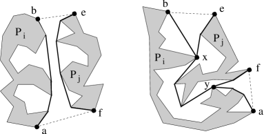
Consider an hourglass $H_{C}$ of a corridor $C$. We first discuss the case when $H_{C}$ is open (see Fig. 6). $H_{C}$ has two sides. Let $S_{1}(H_{C})$ be an arbitrary side of $H_{C}$. The obstacle vertices on $S_{1}(H_{C})$ all lie on the same obstacle, say $P\in\mathcal{P}$. Let $c$ and $d$ be any two adjacent vertices on $S_{1}(H_{C})$ such that the line segment $\overline{cd}$ is not an edge of $P$ (see the left figure in Fig. 6, with $P=P_{j}$). The region enclosed by $\overline{cd}$ and a boundary portion of $P$ between $c$ and $d$ is called the bay of $P$ and $\overline{cd}$, denoted by $bay(\overline{cd})$, which is a simple polygon. We call $\overline{cd}$ the bay gate.

If the hourglass $H_{C}$ is closed, then let $x$ and $y$ be the two apices of its two funnels. Consider two adjacent vertices $c$ and $d$ on a side of a funnel such that the line segment $\overline{cd}$ is not an obstacle edge. If neither $c$ nor $d$ is a funnel apex, then $c$ and $d$ must both lie on the same obstacle and the segment $\overline{cd}$ also defines a bay with that obstacle as above. However, if either $c$ or $d$ is a funnel apex, say, $x=c$, then $x$ and $d$ may lie on different obstacles. If they both lie on the same obstacle, then they also define a bay; otherwise, we call $\overline{xd}$ the canal gate at $x$ (see Fig. 6). Similarly, there is also a canal gate at the funnel apex $y$, say $\overline{yz}$. Let $P_{i}$ and $P_{j}$ be the two obstacles defining the hourglass $H_{C}$. The region enclosed by $P_{i}$, $P_{j}$, and the two canal gates $\overline{xd}$ and $\overline{yz}$ that contains the corridor path of $H_{C}$ is called the canal of $H_{C}$, denoted by $canal(x,y)$, which is a simple polygon.

It is easy to see that $\mathcal{F}\setminus\mathcal{M}$ consists of all bays and canals thus defined.

To build $\mbox{$S\!P\!M$}(\mathcal{F})$, we need to compute the portion of $\mbox{$S\!P\!M$}(\mathcal{F})$ in all bays and canals since we already have $\mbox{$S\!P\!M$}(\mathcal{M})$. As all bays and canals are connected with $\mathcal{M}$ through their gates, we need to “expand” $\mbox{$S\!P\!M$}(\mathcal{M})$ to all bays/canals through their gates. Henceforth, when saying “compute an SPM for a bay/canal,” we mean “expand $\mbox{$S\!P\!M$}(\mathcal{M})$ into that bay/canal”, and vice versa. Computing an SPM for a bay is a key (i.e., the challenging subproblem). Computing an SPM for a canal uses the algorithm for a bay as a main procedure.

4.3.2 Expanding $\mbox{$S\!P\!M$}(\mathcal{M})$ into Bays and Canals

We discuss the bays first. Consider a bay $bay(\overline{cd})$. If its gate $\overline{cd}$ is in a single cell $C(r)$ of $\mbox{$S\!P\!M$}(\mathcal{M})$ with $r$ as the root, then each point in $bay(\overline{cd})$ has a shortest path to $s$ via $r$. Thus, to construct an SPM for $bay(\overline{cd})$, it suffices to compute an SPM on $bay(\overline{cd})$ with respect to the single point $r$. This can be easily done in linear time (in terms of the number of vertices of $bay(\overline{cd})$) since $bay(\overline{cd})$ is a simple polygon. Note that although $r$ may not be a vertex of $bay(\overline{cd})$, we can, for example, connect $r$ to both $c$ and $d$ with two line segments (both $\overline{rc}$ and $\overline{rd}$ are in $C(r)$) to obtain a new simple polygon that contains $bay(\overline{cd})$.

If the gate $\overline{cd}$ is not contained in a single cell of $\mbox{$S\!P\!M$}(\mathcal{M})$, then the situation is more complicated. In this case, multiple vertices of $\mbox{$S\!P\!M$}(\mathcal{M})$ may lie in the interior of $\overline{cd}$ (i.e., the intersections of the boundaries of the cells of $\mbox{$S\!P\!M$}(\mathcal{M})$ with $\overline{cd}$). This is actually the challenging subproblem illustrated by Fig. 1. We refer to the vertices of $\mbox{$S\!P\!M$}(\mathcal{M})$ on $\overline{cd}$ (including its endpoints $c$ and $d$) as the $\mbox{$S\!P\!M$}(\mathcal{M})$ vertices and let $m^{\prime}$ be their total number. Let $n^{\prime}$ be the number of vertices of $bay(\overline{cd})$. A straightforward approach for computing an SPM for $bay(\overline{cd})$ is to use the continuous Dijkstra paradigm [29, 30] to let the wavefront continue to move into $bay(\overline{cd})$. But, this approach may take $O((n^{\prime}+m^{\prime})\log(m^{\prime}+n^{\prime}))$ time. Later in Section 5, we derive an $O(n^{\prime}+m^{\prime})$ time algorithm, as stated below.

Theorem 5

For a bay of $n^{\prime}$ vertices with $m^{\prime}$ $\mbox{$S\!P\!M$}(\mathcal{M})$ vertices on its gate, a shortest path map of size $O(n^{\prime}+m^{\prime})$ for the bay can be computed in $O(n^{\prime}+m^{\prime})$ time.

Since a canal has two gates which are also edges of $\mathcal{M}$, multiple $\mbox{$S\!P\!M$}(\mathcal{M})$ vertices may lie on both its gates. Later in Section 6, we show the following result.

Theorem 6

For a canal of $n^{\prime}$ vertices with totally $m^{\prime}$ $\mbox{$S\!P\!M$}(\mathcal{M})$ vertices on its two gates, a shortest path map of size $O(n^{\prime}+m^{\prime})$ for the canal can be computed in $O(n^{\prime}+m^{\prime})$ time.

4.3.3 Wrapping Things Up

By Theorems 5 and 6, the time bound for computing the shortest path maps for all bays and canals is linear in terms of the total sum of the numbers of obstacle vertices of all bays and canals, which is $O(n)$, and the total number of the $\mbox{$S\!P\!M$}(\mathcal{M})$ vertices on the gates of all bays and canals, which is also $O(n)$ since the size of $\mbox{$S\!P\!M$}(\mathcal{M})$ is $O(n)$.

We hence conclude that given $\mbox{$S\!P\!M$}(\mathcal{M})$, $\mbox{$S\!P\!M$}(\mathcal{F})$ can be computed in additional $O(n)$ time. With a linear size planar point location data structure [13, 26], we have the following result.

Theorem 7

Given a set of $h$ pairwise disjoint polygonal obstacles of totally $n$ vertices and a source point $s$ in the plane, we can build a shortest path map of size $O(n)$ with respect to $s$ in $O(n+h\log^{1+\epsilon}h)$ time (or $O(n+h\log h)$ time if a triangulation of the free space is given) and $O(n)$ space, such that for any query point $t$, the length of a shortest $s$-$t$ path can be reported in $O(\log n)$ time and the actual path can be found in additional $O(k)$ time, where $k$ is the number of turns of the path.

5 Computing a Shortest Path Map for a Bay

Consider a bay $bay(\overline{cd})$ with the gate $\overline{cd}$ (see Fig. 6). Let $\mbox{$S\!P\!M$}(bay(\overline{cd}))$ be the SPM for $bay(\overline{cd})$ that we seek to compute.

For the case when the segment $\overline{cd}$ lies in a single cell $C(r)$ of $\mbox{$S\!P\!M$}(\mathcal{M})$ with the root $r$, we have already shown how to construct $\mbox{$S\!P\!M$}(bay(\overline{cd}))$ in linear time (in terms of the number of vertices of $bay(\overline{cd})$). If the gate $\overline{cd}$ is not contained in a single cell of $\mbox{$S\!P\!M$}(\mathcal{M})$, then let $m^{\prime}$ be the number of $\mbox{$S\!P\!M$}(\mathcal{M})$ vertices on $\overline{cd}$, and $n^{\prime}$ be the number of vertices of $bay(\overline{cd})$. In this section, we give an algorithm for computing $\mbox{$S\!P\!M$}(bay(\overline{cd}))$ in $O(n^{\prime}+m^{\prime})$ time.

Let $R$ be the set of roots of the cells of $\mbox{$S\!P\!M$}(\mathcal{M})$ that intersect with $\overline{cd}$. To obtain $\mbox{$S\!P\!M$}(bay(\overline{cd}))$, we can first compute, for each $r\in R$, the Voronoi region $\mbox{$V\!D$}(r)$ inside $bay(\overline{cd})$ such that for any point $t\in\mbox{$V\!D$}(r)$, there is a shortest $s$-$t$ path via $r$; we then compute an SPM on $\mbox{$V\!D$}(r)$ with respect to the single point $r$. Since every $\mbox{$V\!D$}(r)$ is a simple polygonal region in $bay(\overline{cd})$, the shortest path map $\mbox{$S\!P\!M$}(\mbox{$V\!D$}(r),r)$ can be computed in linear time in terms of the number of vertices of $\mbox{$V\!D$}(r)$ (e.g., by using an algorithm in [16, 17]). Thus, the key is to decompose $bay(\overline{cd})$ into Voronoi regions for the roots of $R$, which is exactly the challenging subproblem illustrated by Fig. 1. Denote by $\mbox{$V\!D$}(bay(\overline{cd}))$ this Voronoi diagram decomposition of $bay(\overline{cd})$. We aim to compute $\mbox{$V\!D$}(bay(\overline{cd}))$ in $O(n^{\prime}+m^{\prime})$ time.

Without loss of generality (WLOG), assume that $\overline{cd}$ is positive-sloped, $bay(\overline{cd})$ is on the right of $\overline{cd}$, and the vertex $c$ is higher than $d$ (e.g., $bay(\overline{cd})=B$ in Fig. 1). Other cases can be handled similarly. Let $R=\{r_{1},r_{2},\ldots,r_{k}\}$ be the set of roots of the cells of $\mbox{$S\!P\!M$}(\mathcal{M})$ that intersect with $\overline{cd}$ in the order from $c$ to $d$ along $\overline{cd}$. Note that $R$ may be a multi-set, i.e., two roots $r_{i}$ and $r_{j}$ with $i\neq j$ may refer to the same physical point; but this is not important to our algorithm (e.g., we can view each $r_{i}$ as a physical copy of the same root). Let $c=v_{0},v_{1},\ldots,v_{k}=d$ be the $\mbox{$S\!P\!M$}(\mathcal{M})$ vertices on $\overline{cd}$ ordered from $c$ to $d$ (thus $m^{\prime}=k+1$). Hence, for each $1\leq i\leq k$, the segment $\overline{v_{i-1}v_{i}}$ is on the boundary of the cell $C(r_{i})$ of $\mbox{$S\!P\!M$}(\mathcal{M})$. Note that each cell $C(r_{i})$ is a star-shaped polygon, and for each $1\leq i\leq k-1$, $v_{i}$ lies on the common boundary of $C(r_{i})$ and $C(r_{i+1})$ (i.e., $v_{i}\in C(r_{i})\cap C(r_{i+1})$). To obtain $\mbox{$V\!D$}(bay(\overline{cd}))$, for each $r_{i}\in R$, we need to compute the Voronoi region $\mbox{$V\!D$}(r_{i})$.

Our algorithm can be viewed as an incremental one, i.e., it considers the roots in $R$ one by one. It is commonly known that incremental approaches can construct Voronoi diagrams in quadratic time, or may give good randomized result. In contrast, our algorithm is deterministic and takes only linear time. The success of it hinges on that we can find an order of the roots in $R$ such that by following this order to consider the roots in $R$ incrementally, we are able to compute $\mbox{$V\!D$}(bay(\overline{cd}))$ in linear time. The order is nothing but that of the indices of the roots in $R$ we have defined. With this order, the algorithm is quite simple. However, it is quite challenging to argue its correctness and achieve a linear time implementation. Our strategy is to show that the algorithm implicitly maintains a number of invariants that assure the correctness of the algorithm. For this purpose, we give many observations (in Section 5.2). Additionally, some interesting techniques are also used to implement and simplify the algorithm.

We first give an algorithm overview in Section 5.1.

5.1 Algorithm Sketch

To compute $\mbox{$V\!D$}(bay(\overline{cd}))$, it turns out that we need to deal with the interactions between some rays, each of which belongs to the bisector of two roots in $R$. Every such ray is either horizontal or vertical. Further, considering the roots in $R$ incrementally is equivalent to considering the corresponding rays incrementally. We process these rays in a certain order (e.g., as to be proved, their origins somehow form a staircase structure). For each ray considered, if it is vertical, then it is easy (it eventually leads to a ray shooting operation), and its processing does not introduce any new ray. But, if it is horizontal, then the situation is more complicated since its processing may introduce many new horizontal rays and (at most) one vertical ray, also in a certain order along a staircase structure (in addition to causing a ray shooting operation). A stack is used to store certain vertical rays that need to be further processed.

The algorithm needs to perform ray shooting operations for some vertical and horizontal rays. Although there are known data structures for ray shooting queries [4, 5, 16, 18], they are not efficient enough for a linear time implementation of the entire algorithm. Based on observations, our approach makes use of the horizontal visibility map and vertical visibility map of $bay(\overline{cd})$ [3]. More specifically, we prove that all vertical ray shootings are in a “nice” sorted order (called target-sorted). With this property, all vertical ray shootings are performed in totally linear time by using the vertical visibility map of $bay(\overline{cd})$. The horizontal visibility map is used to guide the overall process of the algorithm. During the algorithm, we march into the bay and the horizontal visibility map allows us to keep track of our current position (i.e., in a trapezoid of the map that contains our current position). The horizontal visibility map also allows each horizontal ray shooting to be done in $O(1)$ time. In addition, in the preprocessing of the algorithm, we also need to perform some other ray shootings (for rays of slope $-1$); our linear time solution for this also hinges on the target-sorted property of such rays.

Our algorithm is conceptually simple. As mentioned above, the only data structures we need are linked lists, a stack, and the horizontal and vertical visibility maps. Its correctness relies on the fact that the algorithm implicitly maintains a set of invariant properties in each iteration. To prove the algorithmic correctness, of course, we need to show that these invariant properties hold iteratively. Specifically, in our discussion of the algorithm, after each iteration we formally prove that the invariants are well maintained. For this purpose, before presenting the algorithm in Section 5.3, we first show a set of observations in Section 5.2, which capture some essential properties of this $L_{1}$ problem. These observations may be helpful for solving other related problems as well. However, the discussion of these observations and the formal proofs that the invariant properties are maintained by the algorithm somehow make the presentation of this whole section lengthy, technically complicated, or even tedious, for which we ask for the reader’s patience.

5.2 Observations

In this subsection, we give a number of observations, most of which help capture the behaviors of the bisectors for the roots of $R$ in computing $\mbox{$V\!D$}(bay(\overline{cd}))$. Although some of the observations individually might appear simple, they are essential and adding them up leads to an efficient algorithmic strategy for computing $\mbox{$V\!D$}(bay(\overline{cd}))$ (as presented in Section 5.3). The observations also allow our algorithm to perform some key operations (e.g., ray shootings) in a faster manner than using a standard approach [4, 5, 16, 18].

For a point $p$, denote by $x(p)$ its $x$-coordinate and by $y(p)$ its $y$-coordinate. For two objects $O_{1}$ and $O_{2}$ in the plane, if $x(p_{1})\leq x(p_{2})$ for any two points $p_{1}\in O_{1}$ and $p_{2}\in O_{2}$, then we say $O_{1}$ is to the left or west of $O_{2}$, or $O_{2}$ is to the right or east of $O_{1}$; if $y(p_{1})\leq y(p_{2})$ for any two points $p_{1}\in O_{1}$ and $p_{2}\in O_{2}$, then we say $O_{1}$ is to the south of $O_{2}$ or $O_{1}$ is below $O_{2}$, or $O_{2}$ is to the north of $O_{1}$ or $O_{2}$ is above $O_{1}$. If $O_{1}$ is to the left of $O_{2}$ and is also below $O_{2}$, then we say $O_{1}$ is to the southwest of $O_{2}$ or $O_{2}$ is to the northeast of $O_{1}$. We define southeast and northwest similarly.

Figure 7: Illustrating some cases of the bisector $B(p_{1},p_{2})$ of two weighted points $p_{1}$ and $p_{2}$. In (3), an entire quadrant (the shaded area) can be used as $B(p_{1},p_{2})$, but we choose $B(p_{1},p_{2})$ to be the vertical (solid thick) half-line.

In our problem, each root $r_{i}\in R$ can be viewed as an additively weighted point whose weight is the $L_{1}$ length of a shortest path from $s$ to $r_{i}$. Thus, we need to consider the possible shapes of the bisector of two weighted points. For two weighted points $p_{1}$ and $p_{2}$ with weights $w_{1}$ and $w_{2}$, respectively, their bisector $B(p_{1},p_{2})$ consists of all points $q$ such that the $L_{1}$ length of the line segment $\overline{p_{1}q}$ plus $w_{1}$ is equal to the $L_{1}$ length of $\overline{p_{2}q}$ plus $w_{2}$. Figure 7 shows some cases. Note that the bisector can be an entire quadrant of the plane (e.g., see Figure 7(3)); in this case, as in [29, 30], we choose a vertical half-line as the bisector. For any pair of consecutive roots $r_{i-1}$ and $r_{i}$ in $R$ for $2\leq i\leq k$, since the $\mbox{$S\!P\!M$}(\mathcal{M})$ vertex $v_{i-1}\in\overline{cd}$ is on the common boundary of $C(r_{i-1})$ and $C(r_{i})$, $v_{i-1}$ lies on the bisector $B(r_{i-1},r_{i})$ of $r_{i-1}$ and $r_{i}$. For two points $p_{1}$ and $p_{2}$, denote by $Rec(p_{1},p_{2})$ the rectangle with $p_{1}$ and $p_{2}$ as its two diagonal vertices. The next observation is self-evident.

Observation 2

The bisector $B(p_{1},p_{2})$ consists of three portions: Two half-lines and a line segment connecting them; the line segment has a slope $1$ or $-1$ and is the intersection of $B(p_{1},p_{2})$ and the rectangle $Rec(p_{1},p_{2})$, and each of the two half-lines is perpendicular to an edge of $Rec(p_{1},p_{2})$ that touches the half-line. Depending on the relative positions and weights of $p_{1}$ and $p_{2}$, some portions of $B(p_{1},p_{2})$ may degenerate and become empty. $B(p_{1},p_{2})$ is monotone to both the $x$- and $y$-axes. For any line $l$ containing a portion of $B(p_{1},p_{2})$, $p_{1}$ and $p_{2}$ cannot lie strictly on the same side of $l$.

We call the open line segment of $B(p_{1},p_{2})$ strictly inside $Rec(p_{1},p_{2})$ its middle segment, denoted by $B_{M}(p_{1},p_{2})$, and the two half-lines of $B(p_{1},p_{2})$ its two rays, each originating at a point on an edge of $Rec(p_{1},p_{2})$. Thus, the origins of the two rays of $B(p_{1},p_{2})$ are the two endpoints of $B_{M}(p_{1},p_{2})$.

Since each cell in an SPM is a star-shaped simple polygon, the observation below is obvious.

Observation 3

Let $C(r)$ and $C(r^{\prime})$ be two different cells in $\mbox{$S\!P\!M$}(\mathcal{M})$ with roots $r$ and $r^{\prime}$. For any two points $p\in C(r)$ and $p^{\prime}\in C(r^{\prime})$, the line segments $\overline{pr}$ and $\overline{p^{\prime}r^{\prime}}$ cannot cross each other.

The next lemma shows the possible relative positions of two consecutive roots in $R$.

Lemma 6

For any two consecutive roots $r_{i-1}$ and $r_{i}$ in $R$ with $2\leq i\leq k$, $r_{i}$ cannot be to the northeast of $r_{i-1}$, or equivalently, $r_{i-1}$ cannot be to the southwest of $r_{i}$.

Proof: Since the $\mbox{$S\!P\!M$}(\mathcal{M})$ vertex $v_{i-1}\in\overline{cd}$ lies on the common boundary of the two cells $C(r_{i-1})$ and $C(r_{i})$, $v_{i-1}$ is on the bisector $B(r_{i-1},r_{i})$.

Figure 8: An example of $r_{i}$ to the northeast of $r_{i-1}$. The point $p\neq v_{i-1}$ is on $\overline{v_{i-1}v_{i}}$ and is infinitely close to $v_{i-1}$. The line segment $\overline{r_{i}p}$ must cross $\overline{r_{i-1}v_{i-1}}$.

Assume to the contrary that $r_{i}$ is to the northeast of $r_{i-1}$. Note that $v_{i-1}$ may lie on either a half-line or the middle segment of $B(r_{i-1},r_{i})$. In either case, since $r_{i}$ is to the northeast of $r_{i-1}$ and $\overline{cd}$ is positive-sloped, according to Observation 2, $v_{i-1}$ must be lower than $r_{i}$, and $v_{i-1}$ must be to the right of $r_{i-1}$ (see Fig. 8).

Since the segment $\overline{v_{i-1}v_{i}}$ is not a single point and $v_{i}$ is to the left of $v_{i-1}$, we can find a point $p\in\overline{v_{i-1}v_{i}}$ such that $p\neq v_{i-1}$ and $p$ is infinitely close to $v_{i-1}$ (see Fig. 8). Since $p\in\overline{v_{i-1}v_{i}}$ and $\overline{v_{i-1}v_{i}}\subseteq C(r_{i})$, we have $p\in C(r_{i})$. Note that $v_{i-1}\in C(r_{i-1})\cap C(r_{i})$. Below we show that the two line segments $\overline{r_{i}p}$ and $\overline{r_{i-1}v_{i-1}}$ must cross each other, which contradicts with Observation 3.

Since both $r_{i}$ and $r_{i-1}$ are obstacle vertices, by our assumption, $r_{i}$ and $r_{i-1}$ do not lie on a horizontal or vertical line. Hence $r_{i}$ is strictly to the northeast of $r_{i-1}$. Note that no root in $R$ lies on $\overline{cd}$. Since $v_{i-1}$ is lower than $r_{i}$ and is to the right of $r_{i-1}$, the three points $v_{i-1}$, $r_{i}$, and $r_{i-1}$ do not lie on the same line (see Fig. 8). In other words, the triangle $\triangle r_{i}v_{i-1}r_{i-1}$ is a proper one. Further, suppose $\rho(r_{i},v_{i-1})$ (resp., $\rho(r_{i},r_{i-1})$) is the ray originating from $r_{i}$ and going through $v_{i-1}$ (resp., $r_{i-1}$); then $\rho(r_{i},r_{i-1})$ can be obtained by rotating $\rho(r_{i},v_{i-1})$ clockwise by an angle $\angle v_{i-1}r_{i}r_{i-1}>0^{\circ}$. By the definition of the point $p$, during this rotation, $p$ will be encountered by the rotating ray $\rho(r_{i},v_{i-1})$ at an angle $\angle v_{i-1}r_{i}p$ with $0^{\circ}<\angle v_{i-1}r_{i}p<\angle v_{i-1}r_{i}r_{i-1}$, which implies that $\overline{r_{i}p}$ crosses $\overline{r_{i-1}v_{i-1}}$. The lemma thus follows. $\Box$

By Lemma 6, there are three cases on the possible relative positions of $r_{i-1}$ with respect to $r_{i}$, i.e., $r_{i-1}$ can be to the southeast, northwest, or northeast of $r_{i}$.

Lemma 7

Consider any two consecutive roots $r_{i-1}$ and $r_{i}$ in $R$ with $2\leq i\leq k$.

1. If $r_{i}$ is to the southeast of $r_{i-1}$, then $v_{i-1}$ is on a ray of $B(r_{i-1},r_{i})$ that is horizontally going east and $v_{i-1}$ is to the right of $Rec(r_{i-1},r_{i})$ (see Fig. 9(1)).

2. If $r_{i}$ is to the northwest of $r_{i-1}$, then $v_{i-1}$ is on a ray of $B(r_{i-1},r_{i})$ that is vertically going south and $v_{i-1}$ is below $Rec(r_{i-1},r_{i})$ (see Fig. 9(2)).

3. If $r_{i}$ is to the southwest of $r_{i-1}$, then $v_{i-1}$ is either on the middle segment $B_{M}(r_{i-1},r_{i})$, or on a ray of $B(r_{i-1},r_{i})$ that is either horizontally going east or vertically going south (see Fig. 9(3)). Further, if $v_{i-1}$ is on the ray horizontally going east, then $v_{i-1}$ is to the right of $Rec(r_{i-1},r_{i})$; if $v_{i-1}$ is on the ray vertically going south, then $v_{i-1}$ is below $Rec(r_{i-1},r_{i})$.

Proof: We first prove Part 1 of the lemma. If $r_{i}$ is to the southeast of $r_{i-1}$ (see Fig. 9(1)), then the rectangle $Rec(r_{i-1},r_{i})$ cannot intersect $\overline{cd}$. Thus, $v_{i-1}$ cannot be on $B_{M}(r_{i-1},r_{i})$, and $v_{i-1}$ must be on a ray of $B(r_{i-1},r_{i})$, denoted by $\rho$. By Observation 2, the origin of $\rho$ is on an edge $\alpha$ of $Rec(r_{i-1},r_{i})$ and is perpendicular to the edge $\alpha$. Since $v_{i-1}\in\rho$ and $r_{i-1}$ is to the northwest of $r_{i}$, $\alpha$ must be one of the two edges incident to $r_{i}$, i.e., the bottom edge or the right edge of $Rec(r_{i-1},r_{i})$. In addition, if $\alpha$ is the bottom edge of $Rec(r_{i-1},r_{i})$, then $\rho$ must be vertically going south; further, since $r_{i}$ is to the southeast of $r_{i-1}$, by a similar argument as that for the proof of Lemma 6, we can obtain a contradiction. Thus, $\alpha$ is the right edge of $Rec(r_{i-1},r_{i})$ and $\rho$ must be horizontally going east. In addition, it is easy to see that $v_{i-1}$ must be to the right of $Rec(r_{i-1},r_{i})$. Part 1 of the lemma thus follows.

Figure 9: Illustrating the three possible relative positions of $r_{i-1}$ and $r_{i}$.

Part 2 can be proved analogously as Part 1, and we omit it.

For Part 3, if $Rec(r_{i-1},r_{i})$ intersects $\overline{cd}$, then it is possible that $B_{M}(r_{i-1},r_{i})$ intersects $\overline{cd}$ (at $v_{i-1}$). If $B_{M}(r_{i-1},r_{i})$ doest not intersect $\overline{cd}$, then $v_{i-1}$ lies on a ray of $B(r_{i-1},r_{i})$, denoted by $\rho$. Again, the origin of $\rho$ is on either the right edge of $Rec(r_{i-1},r_{i})$ or the bottom edge of $Rec(r_{i-1},r_{i})$. In the former case, $\rho$ is horizontally going east and $v_{i-1}$ is to the right of $Rec(r_{i-1},r_{i})$. In the latter case, $\rho$ is vertically going south and $v_{i-1}$ is below $Rec(r_{i-1},r_{i})$. Part 3 thus follows. $\Box$

For any two consecutive roots $r_{i-1}$ and $r_{i}$ in $R$ with $2\leq i\leq k$, if $v_{i-1}$ is on a ray $\rho$ of $B(r_{i-1},r_{i})$, then we let $\rho_{i-1}$ be the ray originating at $v_{i-1}$ with the same direction as $\rho$. If $v_{i-1}$ lies on the middle segment of $B(r_{i-1},r_{i})$, then by Lemma 7, $r_{i-1}$ is to the northeast of $r_{i}$ and $\overline{cd}$ intersects $Rec(r_{i-1},r_{i})$; in this case, let $\rho_{i-1}$ be the ray of $B(r_{i-1},r_{i})$ that is below or to the right of $v_{i-1}$ and goes inside $bay(\overline{cd})$. For a ray $\rho$, let $or(\rho)$ denote the origin of $\rho$. Observation 4 below is obvious.

Observation 4

For any $2\leq i\leq k$, the ray $\rho_{i-1}$ is either horizontally going east or vertically going south. If $v_{i-1}$ is on a ray of $B(r_{i-1},r_{i})$, then $or(\rho_{i-1})=v_{i-1}$; if $v_{i-1}$ is on $B_{M}(r_{i-1},r_{i})$, then $or(\rho_{i-1})$ is on either the right edge or the bottom edge of $Rec(r_{i-1},r_{i})$.

Lemma 8

Consider any two consecutive roots $r_{i-1}$ and $r_{i}$ in $R$ with $2\leq i\leq k$.

1. If the ray $\rho_{i-1}$ is horizontal, then $r_{i-1}$ is above $\rho_{i-1}$ and $r_{i}$ is below $\rho_{i-1}$.

2. If $\rho_{i-1}$ is vertical, then $r_{i-1}$ is to the right of $\rho_{i-1}$ and $r_{i}$ is to the left of $\rho_{i-1}$.

3. The origin $or(\rho_{i-1})$ of $\rho_{i-1}$ is always below $r_{i-1}$ and to the right of $r_{i}$.

Proof: There are three cases on the possible relative positions of $r_{i-1}$ and $r_{i}$.

• If $r_{i-1}$ is to the northwest of $r_{i}$ (see Fig. 9(1)), then by the proof of Lemma 7, $\rho_{i-1}$ is horizontal and is contained in the ray of $B(r_{i-1},r_{i})$ whose origin is on the right edge of $Rec(r_{i-1},r_{i})$. Since $r_{i-1}$ and $r_{i}$ are two diagonal vertices of $Rec(r_{i-1},r_{i})$, $\rho_{i-1}$ is above $r_{i}$ and below $r_{i-1}$.

  Further, the origin $or(\rho_{i-1})$ is $v_{i-1}$, which is below $r_{i-1}$ and to the right of $r_{i}$.

• If $r_{i-1}$ is to the southeast of $r_{i}$ (see Fig. 9(2)), then by the proof of Lemma 7, $\rho_{i-1}$ is vertical and lies on the ray of $B(r_{i-1},r_{i})$ whose origin is on the bottom edge of $Rec(r_{i-1},r_{i})$. Since $r_{i-1}$ and $r_{i}$ are two diagonal vertices of $Rec(r_{i-1},r_{i})$, $\rho_{i-1}$ is to the right of $r_{i}$ and to the left of $r_{i-1}$. Further, the origin $or(\rho_{i-1})$ is $v_{i-1}$, which is below $r_{i-1}$ and to the right of $r_{i}$.

• If $r_{i-1}$ is to the northeast of $r_{i}$ (see Fig. 9(3)), then if $\rho_{i-1}$ is horizontal, then the proof is similar to the first case; otherwise, the proof is similar to the second case.

The lemma thus follows. $\Box$

Lemma 9

For any $i$ with $3\leq i\leq k-1$, if $r_{i}$ is to the southwest of $r_{i-1}$, then $v_{i-2}$ is to the right of the rectangle $Rec(r_{i-1},r_{i})$ and $v_{i}$ is below $Rec(r_{i-1},r_{i})$.

Proof: Suppose $r_{i}$ is to the southwest of $r_{i-1}$. We only prove that $v_{i-2}$ is to the right of the rectangle $Rec(r_{i-1},r_{i})$. The case that $v_{i}$ is below $Rec(r_{i-1},r_{i})$ can be proved analogously.

Note that $v_{i-2}\in B(r_{i-2},r_{i-1})$. We discuss the three possible relative positions of $r_{i-2}$ and $r_{i-1}$. By Lemma 6, $r_{i-2}$ may be to the southeast, northwest, or northeast of $r_{i-1}$. Since $r_{i}$ is to the southwest of $r_{i-1}$, to prove $v_{i-2}$ is to the right of $Rec(r_{i-1},r_{i})$, it suffices to show that $v_{i-2}$ is to the right of $r_{i-1}$.

• If $r_{i-2}$ is to the southeast of $r_{i-1}$, then by Lemma 7, $v_{i-2}$ is on the ray of $B(r_{i-1},r_{i-2})$ vertically going south, i.e., $\rho_{i-2}$ is vertical. By Lemma 8, $r_{i-1}$ is to the left of $\rho_{i-2}$. Since $v_{i-2}\in\rho_{i-2}$, $v_{i-2}$ is to the right of $r_{i-1}$.

• If $r_{i-2}$ is to the northwest of $r_{i-1}$, then by Lemma 7, $v_{i-2}$ is to the right of $Rec(r_{i-2},r_{i-1})$, and thus to the right of $Rec(r_{i-1},r_{i})$.

• If $r_{i-2}$ is to the northeast of $r_{i-1}$, then the rectangle $Rec(r_{i-2},r_{i-1})$ is to the northeast of $Rec(r_{i-1},r_{i})$. If $v_{i-2}$ is on $B_{M}(r_{i-2},r_{i-1})$, then since $v_{i-2}$ is inside $Rec(r_{i-2},r_{i-1})$, $v_{i-2}$ is to the right of $Rec(r_{i-1},r_{i})$; otherwise, the proof is similar to the above two cases.

The lemma thus follows. $\Box$

Recall that when sketching the algorithm in Section 5.1, we mentioned that the origins of the rays involved somehow form a staircase structure. The next lemma states this important fact.

Lemma 10

For any $i$ with $2\leq i\leq k-1$, $or(\rho_{i-1})$ is to the northeast of $or(\rho_{i})$.

Proof: We first discuss a scenario that will be used later in this proof. Consider any two consecutive roots $r_{j}$ and $r_{j+1}$ in $R$, $1\leq j\leq k-1$, with $or(\rho_{j})\neq v_{j}$. Then based on our discussion above, it must be the case that $r_{j+1}$ is to the southwest of $r_{j}$, $\overline{cd}$ intersects the rectangle $Rec(r_{j},r_{j+1})$, and $or(\rho_{j})$ is a point on an edge of $Rec(r_{j},r_{j+1})$. Let $z_{j}$ be the intersection of $\overline{cd}$ and the right edge of $Rec(r_{j},r_{j+1})$ (see Fig. 10). The origin $or(\rho_{j})$ can be either on the right edge or the bottom edge of $Rec(r_{j},r_{j+1})$. In either case, $or(\rho_{j})$ must be both below and to the left of $z_{j}$, i.e., $z_{j}$ is to the northeast of $or(\rho_{j})$.

Figure 10: Illustrating the case when $r_{j}$ is to the northeast of $r_{j+1}$ and $or(\rho_{j})\neq v_{j}$.

Consider any $i$ with $2\leq i\leq k-1$. To prove the lemma, depending on whether $or(\rho_{i-1})=v_{i-1}$ and whether $or(\rho_{i})=v_{i}$, there are four cases.

1. If $or(\rho_{i-1})=v_{i-1}$ and $or(\rho_{i})=v_{i}$, then since $v_{i-1}$ and $v_{i}$ are on $\overline{cd}$ in the order from $c$ to $d$, $v_{i-1}$ is to the northeast of $v_{i}$, and thus $or(\rho_{i-1})$ is to the northeast of $or(\rho_{i})$.

2. If $or(\rho_{i-1})=v_{i-1}$ and $or(\rho_{i})\neq v_{i}$, then by our discussion at the beginning of this proof, $r_{i+1}$ is to the southwest of $r_{i}$, the rectangle $Rec(r_{i},r_{i+1})$ intersects $\overline{cd}$, and the point $z_{i}$ is to the northeast of $or(\rho_{i})$. Further, since $r_{i+1}$ is to the southwest of $r_{i}$, by Lemma 9, $v_{i-1}$ is to the right of $Rec(r_{i},r_{i+1})$ and thus to the right of $z_{i}$. Since $v_{i-1}$ is to the right of $z_{i}$ and both $v_{i-1}$ and $z_{i}$ are on $\overline{cd}$, $v_{i-1}$ is to the northeast of $z_{i}$. Therefore, $or(\rho_{i-1})$ ($=v_{i-1}$) is to the northeast of $or(\rho_{i})$.

3. If $or(\rho_{i-1})\neq v_{i-1}$ and $or(\rho_{i})=v_{i}$, then the analysis is somewhat similar to the second case.

4. If $or(\rho_{i-1})\neq v_{i-1}$ and $or(\rho_{i})\neq v_{i}$, then $r_{i-1}$ is to the northeast of $r_{i}$ and $r_{i}$ is to the northeast of $r_{i+1}$. Hence, the rectangle $Rec(r_{i-1},r_{i})$ is to the northeast of $Rec(r_{i},r_{i+1})$. Since $or(\rho_{i-1})$ is on $Rec(r_{i-1},r_{i})$ and $or(\rho_{i})$ is on $Rec(r_{i},r_{i+1})$, we also obtain that $or(\rho_{i-1})$ is to the northeast of $or(\rho_{i})$.

The lemma thus follows. $\Box$

Lemma 11

Consider any root $r_{i}\in R$ with $1\leq i\leq k$. For any ray $\rho_{j}$, if $j\leq i-1$ and $\rho_{j}$ is vertical, then $\rho_{j}$ is to the right of $r_{i}$; if $j\geq i$ and $\rho_{j}$ is horizontal, then $\rho_{j}$ is below $r_{i}$.

Proof: WLOG, assume $i<k$. Consider the ray $\rho_{i}$, which is on $B(r_{i},r_{i+1})$. By Lemma 8, the origin $or(\rho_{i})$ is below $r_{i}$. By Lemma 10, for any ray $\rho_{j}$ with $j\geq i$, $or(\rho_{j})$ is below $or(\rho_{i})$ and thus is below $r_{i}$. Hence, if $\rho_{j}$ is horizontal, then $\rho_{j}$ must be below $r_{i}$.

By an analogous analysis, we can show that if $j\leq i-1$ and $\rho_{j}$ is vertical, then $\rho_{j}$ is to the right of $r_{i}$. We omit the details. The lemma thus follows. $\Box$

Note that in any SPM, a common boundary of two adjacent cells $C(r)$ and $C(r^{\prime})$ is a subset of the bisector $B(r,r^{\prime})$.

For any two consecutive roots $r_{i-1}$ and $r_{i}$ in $R$, $2\leq i\leq k$, the vertex $v_{i-1}$ divides $B(r_{i-1},r_{i})$ into two portions; we denote by $B_{bay}(r_{i-1},r_{i})$ the portion that goes inside $bay(\overline{cd})$ following $v_{i-1}$. A key to building $\mbox{$V\!D$}(bay(\overline{cd}))$ is to compute the interactions among all $B_{bay}(r_{i-1},r_{i})$’s, for $i=2,3,\ldots,k$, inside $bay(\overline{cd})$. Note that if $v_{i-1}$ is on a ray of $B(r_{i-1},r_{i})$, then $B_{bay}(r_{i-1},r_{i})$ is the ray $\rho_{i-1}$; otherwise, $v_{i-1}$ is on $B_{M}(r_{i-1},r_{i})$ (i.e., the middle segment of $B(r_{i-1},r_{i})$), and $B_{bay}(r_{i-1},r_{i})$ consists of a portion of $B_{M}(r_{i-1},r_{i})$ in $Rec(r_{i-1},r_{i})$ (i.e., the line segment $\overline{v_{i-1}or(\rho_{i-1})}$) and the ray $\rho_{i-1}$. Lemma 12 below shows that the portion of $B_{M}(r_{i-1},r_{i})$ which is inside $bay(\overline{cd})$ will appear in $\mbox{$S\!P\!M$}(\mathcal{F})$ (and thus in $\mbox{$V\!D$}(bay(\overline{cd}))$), implying that we can simply keep it when computing $\mbox{$V\!D$}(bay(\overline{cd}))$ and we only need to further deal with the rays $\rho_{i}$ for $i=1,2,\ldots,k-1$. Thus, dealing with the rays $\rho_{i}$ is the main issue of our algorithm (as discussed in Section 5.1).

Lemma 12

For any two consecutive roots $r_{i-1}$ and $r_{i}$ in $R$, $2\leq i\leq k$, if $v_{i-1}$ lies on $B_{M}(r_{i-1},r_{i})$, then the portion of $B_{M}(r_{i-1},r_{i})$ inside $bay(\overline{cd})$ will appear in $\mbox{$V\!D$}(bay(\overline{cd}))$.

Proof: Consider two consecutive roots $r_{i-1}$ and $r_{i}$ in $R$, $2\leq i\leq k$, with $v_{i-1}$ lying on $B_{M}(r_{i-1},r_{i})$.

Denote by $B_{M}^{\prime}$ the portion of $B_{M}(r_{i-1},r_{i})$ inside $bay(\overline{cd})$. Recall that $B_{M}(r_{i-1},r_{i})$ is an open segment that does not contain its endpoints and is strictly inside $Rec(r_{i-1},r_{i})$. To prove the lemma, it suffices to show that for any two roots $r_{j}$ and $r_{h}$ in $R$ with $\{r_{j},r_{h}\}\neq\{r_{i-1},r_{i}\}$, if a portion of $B(r_{j},r_{h})$ appears in $\mbox{$S\!P\!M$}(\mathcal{F})$, then that portion does not intersect $B_{M}^{\prime}$.

By Lemma 6, $r_{i}$ may be to the southeast, or northwest, or southwest of $r_{i-1}$. Since $\overline{cd}$ is positive-sloped, if $r_{i}$ is to the northwest or southeast of $r_{i-1}$, then $\overline{cd}$ cannot intersect the rectangle $Rec(r_{i-1},r_{i})$ and thus $v_{i-1}$ cannot lie on $B_{M}(r_{i-1},r_{i})$. Therefore, the only possible case is that $r_{i}$ is to the southwest of $r_{i-1}$.

First, we assume $i-1\geq 2$ and consider the root $r_{i-2}$. We discuss the possible relative positions of $r_{i-2}$ with respect to $r_{i-1}$. Recall that the bisector portion $B_{bay}(r_{i-2},r_{i-1})$ either is $\rho_{i-2}$ or consists of $\overline{v_{i-2}or(\rho_{i-2})}$ and $\rho_{i-2}$. Note that in either case, when moving along $B_{bay}(r_{i-2},r_{i-1})$ from $v_{i-2}$, $B_{bay}(r_{i-2},r_{i-1})$ is monotonically increasing in the $x$-coordinates. Hence, $v_{i-2}$ is a leftmost point of $B_{bay}(r_{i-2},r_{i-1})$. Since $r_{i}$ is to the southwest of $r_{i-1}$, by Lemma 9, $v_{i-2}$ is to the right of $Rec(r_{i-1},r_{i})$ and thus is strictly to the right of $B_{M}^{\prime}$. Hence, $B_{bay}(r_{i-2},r_{i-1})$ cannot intersect $B_{M}^{\prime}$.

For any pair of consecutive roots $r_{j-1}$ and $r_{j}$ in $R$, $2\leq j\leq i-2$, similarly, when moving from $v_{j-1}$ along $B_{bay}(r_{j-1},r_{j})$, $B_{bay}(r_{j-1},r_{j})$ is monotonically increasing in the $x$-coordinates. Since $v_{i-2}$ is strictly to the right of $B_{M}^{\prime}$ and $v_{j-1}$ is to the right of $v_{i-2}$, $B_{bay}(r_{j-1},r_{j})$ cannot intersect $B_{M}^{\prime}$.

Let $R_{1}=\{r_{1},r_{2},\ldots,r_{i-1}\}$ and $R_{2}=\{r_{i},r_{i+1},\ldots,r_{k}\}$. (Note that since $R$ may be a multi-set, $R_{1}$ and $R_{2}$ possibly contain the same physical root, but this is not important to our analysis.)

For any two different pairs of consecutive roots $r_{j-1},r_{j}$ and $r_{t-1},r_{t}$ with $2\leq j\leq i-1$ and $2\leq t\leq i-1$, it is possible that $B_{bay}(r_{j-1},r_{j})$ and $B_{bay}(r_{t-1},r_{t})$ intersect in $\mbox{$S\!P\!M$}(\mathcal{F})$; if that happens, then let $B^{\prime}$ be the resulting bisector. It is not difficult to see that $B^{\prime}$ must be going in a direction between the original directions of $B_{bay}(r_{j-1},r_{j})$ and $B_{bay}(r_{t-1},r_{t})$. Since neither $B_{bay}(r_{j-1},r_{j})$ nor $B_{bay}(r_{t-1},r_{t})$ intersects $B_{M}^{\prime}$, $B^{\prime}$ cannot intersect $B_{M}^{\prime}$. We can further consider the possible intersection between $B^{\prime}$ and the bisector of another two roots in $R_{1}$ in the manner as above, and show likewise that the new bisector thus resulted cannot intersect $B_{M}^{\prime}$.

The above argument shows that for any two roots $r_{j}$ and $r_{t}$ in $R_{1}$ such that a portion of $B(r_{j},r_{t})$ appears in $\mbox{$V\!D$}(bay(\overline{cd}))$, that portion does not intersect $B_{M}^{\prime}$. By a similar argument, we can also show that for any two roots $r_{j}$ and $r_{t}$ in $R_{2}$ such that a portion of $B(r_{j},r_{t})$ appears in $\mbox{$V\!D$}(bay(\overline{cd}))$, that portion does not intersect $B_{M}^{\prime}$.

It remains to show that for any two roots $r_{j}\in R_{1}$ and $r_{t}\in R_{2}$ such that $\{r_{j},r_{t}\}\neq\{r_{i-1},r_{i}\}$ and a portion of $B(r_{j},r_{t})$ appears in $\mbox{$V\!D$}(bay(\overline{cd}))$, that portion does not intersect $B_{M}^{\prime}$. Note that the case of $B(r_{j},r_{t})$ (partially) appearing in $\mbox{$V\!D$}(bay(\overline{cd}))$ can occur only after $B_{bay}(r_{i-1},r_{i})$ is “blocked” by an intersection between $B_{bay}(r_{i-1},r_{i})$ and the bisector of two roots in $R_{1}$ or two roots in $R_{2}$. Since the bisector of any two roots in $R_{1}$ or any two roots in $R_{2}$ cannot intersect $B_{M}^{\prime}$, the portion of $B(r_{j},r_{t})$ appearing in $\mbox{$V\!D$}(bay(\overline{cd}))$ cannot intersect $B^{\prime}_{M}$ either.

The lemma thus follows. $\Box$

The observations presented above help determine the behaviors of the bisectors for the roots in $R$ (e.g., the properties of the rays $\rho_{1},\rho_{2},\ldots,\rho_{k-1}$), which are crucial to constructing $\mbox{$V\!D$}(bay(\overline{cd}))$. They form a basis for both showing the correctness and the efficiency of our algorithm in Section 5.3. For example, Lemma 10 can help conduct a set of ray shooting operations in linear time, and Lemma 12 allows us to decompose the problem into certain subproblems with good properties.

5.3 The Algorithm for Computing $\mbox{$V\!D$}(bay(\overline{cd}))$

In this subsection, we present our algorithm for computing $\mbox{$V\!D$}(bay(\overline{cd}))$, i.e., computing the Voronoi region $\mbox{$V\!D$}(r)$ for each root $r\in R$.

As shown in [29, 30], a key property of the problem in the $L_{1}$ metric is: There exists an SPM such that each edge of the SPM is horizontal, or vertical, or of a slope $1$ or $-1$. As shown below, the curves involved in specifying $\mbox{$V\!D$}(bay(\overline{cd}))$ consist of only line segments of slopes $0$, $\infty$, and $-1$ (there is no $+1$, which is due to the assumption that $\overline{cd}$ is positive-sloped). A line (segment) is said to be ($-1$)-sloped if its slope is $-1$. Our algorithm needs to perform some vertical, horizontal, and ($-1$)-sloped ray shooting queries, whose total number is $O(k)$. By exploiting some properties of our problem shown in Section 5.2, we conduct all ray shootings in a global manner in totally $O(n^{\prime}+k)$ time.

Input: $bay(\overline{cd})$, $R=\{r_{1},r_{2},\ldots,r_{k}\}$, and $\mbox{$S\!P\!M$}(\mathcal{M})$ vertices $v_{1},v_{2},\ldots,v_{k-1}$.

Output: A shortest path map on $bay(\overline{cd})$ with respect to the source point $s$.

/* Preprocessing */

1 Compute the ray set $\Psi=\{\rho_{1},\rho_{2},\ldots,\rho_{k-1}\}$ ;

2 Compute the line segment $\overline{v_{i}or(\rho_{i})}$ for each $1\leq i\leq k-1$ if $v_{i}\neq or(\rho_{i})$ ;

3 Compute the horizontal visibility map $\mbox{$H\!M$}(bay(\overline{cd}))$ and the vertical visibility map $\mbox{$V\!M$}(bay(\overline{cd}))$ ;

4 Compute the trapezoid in $\mbox{$H\!M$}(bay(\overline{cd}))$ that contains $or(\rho_{i})$ for each $1\leq i\leq k-1$ ;

/* The main algorithm */

$p^{*}\leftarrow c$, $S\leftarrow\emptyset$, $Q\leftarrow\{\rho_{1},\rho_{2},\ldots,\rho_{k-1}\}$ ;

 /* $Q$ is a queue storing the rays. */

5 while $Q$ is not empty do

       Consider the first ray $\rho$ in $Q$ and remove it from $Q$ ;

       /* Assume $\rho$ is on $B(r_{j},r_{i})$ with $i>j$. */

6       if $\rho$ is vertical then

7            Push $\rho$ onto the top of $S$, and exit the current loop ;

8            

9      else /* $\rho$ is horizontal. */

10             Compute the target point $tp(\rho)$ ;

11             if $S$ is empty then

12                  The Voronoi region $\mbox{$V\!D$}(r_{j})$ is determined with $\overline{or(\rho)tp(\rho)}$ ;

13                   $p^{*}\leftarrow tp(\rho)$, and exit the current loop ;

14                  

15            else /* $S$ is not empty; assume $\rho^{\prime}\subset B(r_{t},r_{j})$ with $j>t$ is the ray at the top of $S$. */

16                  Scan $\partial(p^{*},tp(\rho))$ to compute the target points on $\partial(p^{*},tp(\rho))$ of the rays in $S$ ;

17                   if $tp(\rho^{\prime})$ is before $tp(\rho)$ (i.e., $tp(\rho^{\prime})$ has been computed) then

18                         Determine the Voronoi regions for the roots defining the rays in $S$ ;

19                         Pop all rays out of $S$ ;

20                         $p^{*}\leftarrow tp(\rho)$, and exit the current loop ;

21                        

22                  else /* $tp(\rho^{\prime})$ is not before $tp(\rho)$ (i.e., $tp(\rho^{\prime})$ has not been computed). */

23                         Determine the Voronoi region $\mbox{$V\!D$}(r_{j})$ ;

24                         Let $p$ be the intersection of $\rho$ and $\rho^{\prime}$, and $q$ be the intersection of the horizontal line through $r_{i}$ and the vertical line through $r_{t}$; let $p^{\prime}$ be the other intersection of $B_{M}(r_{t},r_{i})$ and the boundary of $Rec(p,q)$ than $p$;

25                         Move from $p$ along $\overline{pp^{\prime}}$ in $\mbox{$H\!M$}(bay(\overline{cd}))$ until either $p^{\prime}$ or $\partial$ is encountered first;

26                         if $\partial$ is encountered (say, at the point $z$) then

27                               Scan $\partial(tp(\rho),z)$ to compute the target points on $\partial(tp(\rho),z)$ of the rays in $S$ ;

28                               Determine the Voronoi regions for the roots defining the rays in $S$ ;

29                               Pop all rays out of $S$ ;

30                               $p^{*}\leftarrow z$, and exit the current loop ;

31                              

32                        else /* $\partial$ is not encountered. */

33                               Pop $\rho^{\prime}$ out of $S$ ;

34                               if $p^{\prime}$ is on the bottom edge of $Rec(p,q)$ then

35                                     Push the ray originating at $p^{\prime}$ and going south onto the top of $S$ ;

36                                    

37                              else /* $p^{\prime}$ is on the right edge of $Rec(p,q)$. */

38                                     Add the ray originating at $p^{\prime}$ and going east to the front of $Q$ ;

39                                    

40                               $p^{*}\leftarrow tp(\rho)$, and exit the current loop ;

41                              

42                        

43                  

44            

45      

46 For each $r_{i}\in\Psi$, compute the SPM on the Voronoi region $\mbox{$V\!D$}(r_{i})$ with respect to $r_{i}$;

Algorithm 1 Computing a shortest path map for $bay(\overline{cd})$

The pseudo-code of Algorithm 1 summarizes the entire algorithm.

Before describing the main algorithm, we discuss some preprocessing work as well as some basic algorithmic methods that will be used later in the main algorithm.

5.3.1 Preliminaries and Preprocessing

By Lemma 12, for any two consecutive roots $r_{i-1}$ and $r_{i}$ in $R$, $2\leq i\leq k$, if the middle segment $B_{M}(r_{i-1},r_{i})$ of their bisector intersects $\overline{cd}$ (at $v_{i-1}$), then we can “separately” process the portion of $B_{M}(r_{i-1},r_{i})$ inside $Rec(r_{i-1},r_{i})$, as follows. Let $\partial$ be the boundary of $bay(\overline{cd})$ minus $\overline{cd}$, i.e., $\partial$ consists of all edges of $bay(\overline{cd})$ except $\overline{cd}$.

Figure 11: Illustrating an example of $B_{M}(r_{i-1},r_{i})$ intersecting both $\overline{cd}$ (at $v_{i-1}$) and $\partial$ (at $p$). The line segment $\overline{v_{i-1}p}$ divides $bay(\overline{cd})$ into $bay_{1}$ and $bay_{2}$.

Clearly, $v_{i-1}$ divides $B_{M}(r_{i-1},r_{i})$ into two portions; one portion does not contain any point in $bay(\overline{cd})$ and the other contains some points in $bay(\overline{cd})$. Denote by $B_{M}^{\prime}(r_{i-1},r_{i})$ the portion that contains some points in $bay(\overline{cd})$. Thus, $B_{M}^{\prime}(r_{i-1},r_{i})$ is a line segment and $v_{i-1}$ is one of its endpoints (and $or(\rho_{i-1})$ is the other endpoint). We first determine whether $B_{M}^{\prime}(r_{i-1},r_{i})$ intersects $\partial$, by performing a $-1$-sloped ray shooting operation. Specifically, we shoot a ray $\rho$ originating at $v_{i-1}$ and passing through the other endpoint of $B_{M}^{\prime}(r_{i-1},r_{i})$. If the length of the portion of $\rho$ between $v_{i-1}$ and the first point $p$ on $\partial$ hit by $\rho$ is larger than the length of $B_{M}^{\prime}(r_{i-1},r_{i})$, then $B_{M}^{\prime}(r_{i-1},r_{i})$ does not intersect $\partial$, and we do nothing. Otherwise, $B_{M}^{\prime}(r_{i-1},r_{i})$ intersects $\partial$ (at the point $p$). By Lemma 12, the line segment $\overline{v_{i-1}p}$ appears in $\mbox{$S\!P\!M$}(\mathcal{F})$. Also, $\overline{v_{i-1}p}$ partitions $bay(\overline{cd})$ into two simple polygons (see Fig. 11); one polygon contains $\overline{cv_{i-1}}$ as an edge, which we denote as $bay_{1}$, and we denote the other polygon as $bay_{2}$. Let $R_{1}=\{r_{1},r_{2},\ldots,r_{i-1}\}$ and $R_{2}=\{r_{i},r_{i+1},\ldots,r_{k}\}$. (Note that since $R$ may be a multi-set, $R_{1}$ and $R_{2}$ possibly refers to the same physical root, but this is not important to our algorithm.) Since $\overline{v_{i-1}p}$ is in $\mbox{$V\!D$}(bay(\overline{cd}))$, it is not difficult to see that for any point $q$ in $bay_{1}$, there is a root $r\in R_{1}$ such that a shortest path from $s$ to $q$ goes through $r$. Similarly, for any point $q$ in $bay_{2}$, there is a root $r\in R_{2}$ such that a shortest $s$-$q$ path goes through $r$. This implies that we can divide the original problem of computing $\mbox{$V\!D$}(bay(\overline{cd}))$ on $bay(\overline{cd})$ and $R$ into two subproblems of computing $\mbox{$V\!D$}(bay_{1})$ on $bay_{1}$ and $R_{1}$ and computing $\mbox{$V\!D$}(bay_{2})$ on $bay_{2}$ and $R_{2}$.

If we process each pair of consecutive roots in $R$ as above, then the original problem may be divided into multiple subproblems, each of which has the following property: For any pair of consecutive roots $r_{i-1}$ and $r_{i}$ in the corresponding root subset of $R$, if $B_{M}(r_{i-1},r_{i})$ intersects $\overline{cd}$, then $B^{\prime}_{M}(r_{i-1},r_{i})$ does not intersect $\partial$ and is contained in the corresponding subpolygon of $bay(\overline{cd})$; further, $B^{\prime}_{M}(r_{i-1},r_{i})$ is in $\mbox{$V\!D$}(bay(\overline{cd}))$ and has been computed.

To perform the above process, a key is to derive an efficient method for the $-1$-sloped ray shooting operations. For this, we choose to check all pairs of consecutive roots in $R$ in the order of $r_{1},r_{2},\ldots,r_{k}$. In this way, it is easy to see that the ray shootings are conducted such that the origins of the rays are sorted along $\overline{cd}$ from $c$ to $d$. This is summarized by the next observation.

Observation 5

The preprocessing conducts $O(k)$ $-1$-sloped ray shooting operations that are organized such that the origins of all rays are on $\overline{cd}$ ordered from $c$ to $d$.

We show next that the ray shootings for Observation 5 can be done in $O(n^{\prime}+k)$ time. Since the origins of all rays in Observation 5 are sorted on $\overline{cd}$, we can perform the ray shootings by computing the visible region of $bay(\overline{cd})$ from $\overline{cd}$ along the direction of these rays. This can be easily done by a visibility algorithm on a simple polygon (e.g., [1, 23, 28]). Below, we give a different algorithm for a more general problem; this more general result is needed by the main algorithm.

Given a simple polygon $P$, the horizontal visibility map of $P$ contains a horizontal line segment inside $P$ through each vertex of $P$, extending as long as possible without properly crossing the boundary of $P$ (such line segments are called the diagonals; see Fig. 12). The vertical visibility map with vertical diagonals is defined similarly. Each region in a visibility map is a trapezoid (a triangle is a special trapezoid). A visibility map of a simple polygon can be computed in linear time [3].

Figure 12: Illustrating the horizontal visibility map of a simple polygon.

For a ray $\rho$ with its origin in $bay(\overline{cd})$ (inside it or on the boundary), the boundary point of $bay(\overline{cd})$ that is not the origin $or(\rho)$ hit by $\rho$ first is called the target point of $\rho$, denoted by $tp(\rho)$. Recall that $\partial$ is the boundary of $bay(\overline{cd})$ excluding the edge $\overline{cd}$. In the rest of this paper, unless otherwise stated, a ray in our discussion always has its origin in $bay(\overline{cd})$ and its target point on $\partial$.

We say that $m$ parallel rays $\rho_{1}^{\prime},\rho_{2}^{\prime},\ldots,\rho_{m}^{\prime}$ are target-sorted if we move from $c$ to $d$ (clockwise) on $\partial$, we encounter the target points of these rays on $\partial$ in the order of $tp(\rho^{\prime}_{1}),tp(\rho^{\prime}_{2}),\ldots,tp(\rho^{\prime}_{m})$.

Given a set of $m$ target-sorted parallel rays $\rho_{1}^{\prime},\rho_{2}^{\prime},\ldots,\rho_{m}^{\prime}$ for $bay(\overline{cd})$ whose origins are in $bay(\overline{cd})$ and whose target points are on $\partial$, below we present a visibility map based approach for computing their target points in $O(n^{\prime}+m)$ time (recall that $n^{\prime}$ is the number of vertices of $bay(\overline{cd})$).

WLOG, we assume that the rays are all horizontal. We first compute the horizontal visibility map of $bay(\overline{cd})$ in $O(n^{\prime})$ time. Then, starting from the vertex $c$, we scan $\partial$ and check each edge $e$ of $\partial$ and the trapezoid $t(e)$ of the visibility map bounded by $e$, to see whether the next ray $\rho_{i}^{\prime}$ (initially $i=1$) is in the trapezoid $t(e)$ and can hit the edge $e$. Once the target point of the ray $\rho_{i}^{\prime}$ is found, we continue with the next ray $\rho_{i+1}^{\prime}$. Clearly, the time for computing all target points is $O(n^{\prime}+m)$. Thus, we have the following result.

Lemma 13

Given a set of $m$ target-sorted parallel rays for $bay(\overline{cd})$ whose origins are in $bay(\overline{cd})$ and whose target points are on $\partial$, their target points can be computed in $O(n^{\prime}+m)$ time.

For the ray shootings in Observation 5, it is easy to see that these rays are target-sorted. Thus, by Lemma 13, their target points can be computed in $O(n^{\prime}+k)$ time (of course, these ray shootings can be done by using the visibility algorithms in [1, 23, 28], which do not compute a visibility map). We present the above visibility map based technique because our main algorithm in Section 5.3.2 will need it.

In addition, as part of the preprocessing for our main algorithm, we also compute the horizontal visibility map $\mbox{$H\!M$}(bay(\overline{cd}))$ and the vertical visibility map $\mbox{$V\!M$}(bay(\overline{cd}))$ of $bay(\overline{cd})$. Further, for each $1\leq i\leq k-1$, we compute the trapezoid of the horizontal visibility map $\mbox{$H\!M$}(bay(\overline{cd}))$ that contains the origin $or(\rho_{i})$ of the ray $\rho_{i}$, in totally $O(n^{\prime}+k)$ time, in the following way.

Recall that $or(\rho_{i})$ is either $v_{i}$ or in the interior of $bay(\overline{cd})$. In the latter case, $or(\rho_{i})$ is an endpoint of the line segment $B^{\prime}_{M}(r_{i},r_{i+1})=\overline{v_{i}or(\rho_{i})}$ whose slope is $-1$, and the position of $or(\rho_{i})$ has been determined earlier by the $-1$-sloped ray shooting operations. By Lemma 10, all origins $or(\rho_{1}),or(\rho_{2}),\ldots,or(\rho_{k-1})$ are ordered from northeast to southwest. Further, $or(\rho_{i})$’s are all visible from $\overline{cd}$ along the direction of slope $-1$. Thus, it is not difficult to show that if we visit the trapezoids of $\mbox{$H\!M$}(bay(\overline{cd}))$ by scanning the edges of $\partial$ from $c$ to $d$ and looking at the trapezoids bounded by each edge, then the trapezoids containing such $or(\rho_{i})$’s are encountered in the same order as $or(\rho_{1}),or(\rho_{2}),\ldots,or(\rho_{k-1})$. This implies that we can use a similar algorithm as for computing the target points of target-sorted parallel rays on $\partial$ (i.e., scanning $\partial$ from $c$ to $d$ and checking the trapezoids of $\mbox{$H\!M$}(bay(\overline{cd}))$ thus visited along $\partial$) to find all the sought trapezoids, in $O(n^{\prime}+k)$ time.

The above discussion leads to the following lemma.

Lemma 14

The preprocessing on $bay(\overline{cd})$ takes $O(n^{\prime}+k)$ time.

In the main algorithm, the horizontal visibility map $\mbox{$H\!M$}(bay(\overline{cd}))$ will be used to guide the main process. More specifically, during the algorithm, we traverse inside $bay(\overline{cd})$ following certain rays, and use $\mbox{$H\!M$}(bay(\overline{cd}))$ to keep track of where we are (i.e., which trapezoid of $\mbox{$H\!M$}(bay(\overline{cd}))$ contains our current position). The vertical visibility map $\mbox{$V\!M$}(bay(\overline{cd}))$ will be used to compute the target points of some target-sorted vertical rays using the above visibility map based approach.

For any two points $a$ and $b$ on $\partial$ with $a$ lying on the portion of $\partial$ from $c$ clockwise to $b$, we denote by $\partial(a,b)$ the portion of $\partial$ between $a$ and $b$ and say that $a$ is before $b$ or $b$ is after $a$.

5.3.2 The Main Algorithm

After the preprocessing, the problem of computing $\mbox{$V\!D$}(bay(\overline{cd}))$ with the root set $R$ may be divided into multiple subproblems and we need to solve each subproblem. For convenience of the forthcoming discussion, we assume that the original problem on $bay(\overline{cd})$ with $R$ is merely one such subproblem, i.e., for any two consecutive roots $r_{i}$ and $r_{i+1}$ in $R$, if $v_{i}\in B_{M}(r_{i},r_{i+1})$, then $B^{\prime}_{M}(r_{i},r_{i+1})$ ($=\overline{v_{i}or(\rho_{i})}$) lies completely in $\mbox{$V\!D$}(bay(\overline{cd}))$ and has been computed. Recall that in the preprocessing, we have already computed the trapezoid of the horizontal visibility map $\mbox{$H\!M$}(bay(\overline{cd}))$ that contains the origin $or(\rho_{i})$ of the ray $\rho_{i}$, for each $1\leq i\leq k-1$. Observation 6 below summarizes these facts.

Observation 6

After the preprocessing,

• for any two consecutive roots $r_{i}$ and $r_{i+1}$ in $R$, if $v_{i}\in B_{M}(r_{i},r_{i+1})$, then their bisector portion $B^{\prime}_{M}(r_{i},r_{i+1})$ ($=\overline{v_{i}or(\rho_{i})}$) has been computed;

• for each $1\leq i\leq k-1$, the trapezoid of $\mbox{$H\!M$}(bay(\overline{cd}))$ that contains the origin $or(\rho_{i})$ of the ray $\rho_{i}$ is known.

As discussed before, our task is to handle the interactions among the rays $\rho_{i}$ for all $i=1,2,\ldots,k-1$.

In the algorithm, we need to compute the target points for $O(k)$ horizontal and vertical rays. The main procedure is guided by the horizontal visibility map $\mbox{$H\!M$}(bay(\overline{cd}))$ so that the target point of each horizontal ray can be determined in constant time. For the vertical ray shootings, we use the visibility map based approach with the vertical visibility map $\mbox{$V\!M$}(bay(\overline{cd}))$. Note that the vertical ray shootings will occur in an online fashion in the algorithm. We will show that the vertical rays involved are target-sorted. To compute the target points for these vertical rays, the algorithm maintains a reference point, denoted by $p^{*}$. Initially, $p^{*}=c$. Then during the algorithm, $p^{*}$ will be moved forward along $\partial$ from $c$ to $d$, i.e., every time $p^{*}$ is moved on $\partial$, its new position is always after its previous position. In this way, the target points of all vertical rays are computed in totally $O(n^{\prime}+k)$ time (recall that $n^{\prime}$ is the number of obstacle vertices of $bay(\overline{cd})$).

Let $\Psi=\{\rho_{1},\rho_{2},\ldots,\rho_{k-1}\}$. We process the rays of $\Psi$ incrementally in the order of $\rho_{1},\rho_{2},\ldots,\rho_{k-1}$, whose origins are ordered from northeast to southwest by Lemma 5 10. By Observation 4, each ray in $\Psi$ is either horizontally going east or vertically going south. We say that initially all rays are active and the entire $bay(\overline{cd})$ is active. In general, the active rays are used to decompose the active region of $bay(\overline{cd})$. During the algorithm, some portion of $bay(\overline{cd})$ will be implicitly set as inactive, which means that each point of such a region is in the Voronoi region of a root that has been determined. The active region of $bay(\overline{cd})$ at any moment of the algorithm always forms a connected simple polygon, a fact that we will not explicitly argue in the following algorithm description. Similarly, some rays will be set as inactive, meaning that they will no longer be involved in the further decomposition of the current active region of $bay(\overline{cd})$. When the algorithm terminates, the entire $bay(\overline{cd})$ is inactive and all rays of $\Psi$ are inactive. Note that setting a region or a ray as inactive is done implicitly and is used only for our analysis. Since each ray in $\Psi$ lies on the bisector of two roots in $R$, we say that the two roots define the ray.

Figure 13: Illustrating an example of $\rho_{1}$ being horizontal.

We start with the first ray $\rho_{1}$. If $\rho_{1}$ is horizontal (going east), then since $or(\rho_{1})$ is the most northeast origin, no other ray in $\Psi$ can intersect it. Let $p$ be the target point of $\rho_{1}$ on $\partial$ (see Fig. 13). Clearly, $p$ can be found in $O(1)$ time since we already know the trapezoid in $\mbox{$H\!M$}(bay(\overline{cd}))$ that contains $or(\rho_{1})$ by Observation 6. Denote by $\alpha$ the portion of $B(r_{1},r_{2})$ between $v_{1}$ and $p$. Note that $\alpha$ is either the line segment $\overline{v_{1}p}$ (if $v_{1}=or(\rho_{1})$), or the concatenation of the two line segments $\overline{v_{1}or(\rho_{1})}$ and $\overline{or(\rho_{1})p}$. In either case, $\alpha$ partitions $bay(\overline{cd})$ into two simple polygons. One of them contains $\overline{cv_{1}}$ as an edge and we denote it by $bay_{1}$ (see Fig. 13). We claim that $bay_{1}$ is the Voronoi region of $r_{1}$, i.e., $\mbox{$V\!D$}(r_{1})=bay_{1}$. Indeed, by the above analysis and Lemma 12, $\alpha$ is in $\mbox{$V\!D$}(bay(\overline{cd}))$, implying that for any point $q\in bay_{1}$, there is a shortest path from $s$ to $q$ via $r_{1}$. The claim thus follows, and $\mbox{$V\!D$}(r_{1})$ is determined. We then set the ray $\rho_{1}$ and the region of $bay_{1}$ as inactive. Hence, the active region of $bay(\overline{cd})$ becomes $bay(\overline{cd})\setminus bay_{1}$, which needs to be further decomposed. In addition, we move the reference point $p^{*}$ from $c$ to $p$ ($=tp(\rho_{1})$). We then continue with the next ray $\rho_{2}$.

If $\rho_{1}$ is vertical (going south), then we push $\rho_{1}$ onto a stack $S$ (initially, $S=\emptyset$), and let the reference point $p^{*}$ stay at $c$. We then continue with the next ray $\rho_{2}$.

We will show below that our algorithm maintains the following general invariants, which are used to prove the correctness of the algorithm. Suppose the current moment of the algorithm is right before the next ray $\rho$ is considered, and assume $\rho$ lying on the bisector $B(r_{j},r_{i})$ with $i>j$. The stack $S$ may be non-empty; if $S=\emptyset$, then the invariants below related to any rays in $S$ are not applicable. Let $\rho^{\prime}$ be the ray at the top of $S$, and suppose $\rho^{\prime}$ lies on $B(r_{t},r_{t^{\prime}})$ with $t^{\prime}>t$.

Invariant Properties: (1) All rays in $S$ are active and vertically going south. (2) The origins of all rays in $S$ from top to bottom are ordered from southwest to northeast. (3) The origin of the next ray to be considered by the algorithm (i.e., $\rho$) is to the southwest of the origin of the ray at the top of $S$ (i.e., $\rho^{\prime}$). (4) The two indices $j=t^{\prime}$. (5) For each ray $\rho^{\prime\prime}$ in $S\cup\{\rho\}$, suppose $\rho^{\prime\prime}$ lies on the bisector $B(r_{j^{\prime}},r_{i^{\prime}})$ of two roots $r_{j^{\prime}}$ and $r_{i^{\prime}}$ with $i^{\prime}>j^{\prime}$; then the portion of the boundary of the Voronoi region $\mbox{$V\!D$}(r_{i^{\prime}})$ (resp., $\mbox{$V\!D$}(r_{j^{\prime}})$) from $v_{i^{\prime}-1}$ (resp., $v_{j^{\prime}}$) to the origin $or(\rho^{\prime\prime})$ of $\rho^{\prime\prime}$ has already been computed. (6) For each ray $\rho^{\prime\prime}$ in $S$, suppose it lies on the bisector $B(r_{j^{\prime}},r_{i^{\prime}})$ of two roots $r_{j^{\prime}}$ and $r_{i^{\prime}}$ with $i^{\prime}>j^{\prime}$; then $r_{j^{\prime}}$ is to the right of $\rho^{\prime\prime}$ and $r_{i^{\prime}}$ is to the left of $\rho^{\prime\prime}$. (7) The root $r_{t}$ is to the left of all rays in $S\setminus\{\rho^{\prime}\}$ (recall that $\rho^{\prime}\subset B(r_{t},r_{t^{\prime}})$ with $t^{\prime}>t$). (8) For any two consecutive rays $\rho^{\prime}_{1}$ and $\rho^{\prime}_{2}$ in $S$ such that $\rho^{\prime}_{1}$ is closer to the top of $S$, suppose $\rho^{\prime}_{1}$ is on $B(r_{i_{1}},r_{i_{2}})$ for $i_{2}>i_{1}$ and $\rho^{\prime}_{2}$ is on $B(r_{j_{1}},r_{j_{2}})$ for $j_{2}>j_{1}$; then $i_{1}=j_{2}$. (9) The target points of all rays in $S$ from bottom to top are ordered clockwise on $\partial$ (i.e., from $c$ to $d$). (10) If $\rho$ is vertical, then the target point $tp(\rho)$ of $\rho$ is after the target point $tp(\rho^{\prime})$ of $\rho^{\prime}$ on $\partial$. (11) If the target point of any ray in $S$ has not been computed yet, then the target point of that ray is after the reference point $p^{*}$ (i.e., on $\partial(p^{*},d)$). (12) The target point $tp(\rho)$ is after $p^{*}$. (13) Suppose $\rho^{\prime\prime}$ is the first horizontal ray in $\Psi$ that will be considered by the algorithm in a future time from now; then its target point $tp(\rho^{\prime\prime})$ is after $p^{*}$. (14) The trapezoid in the horizontal visibility map $\mbox{$H\!M$}(bay(\overline{cd}))$ that contains the origin $or(\rho)$ of the ray $\rho$ is known.

Now consider the moment that is right after we finish processing $\rho_{1}$ and before we consider $\rho_{2}$. Based on the processing of $\rho_{1}$ discussed above, either $\rho_{1}$ is horizontal and $S$ is empty, or $\rho_{1}$ is vertical and $S=\{\rho_{1}\}$. Lemma 15 below shows that in either case, all invariants of the algorithm hold. We intend to use the proof of Lemma 15 as a “warm-up” for the analysis of the more general situations later. Observation 7 follows from the definitions of the rays in $\Psi$ and Lemma 10.

Observation 7

The target points of all rays in $\Psi$ are on $\partial$. For any two rays $r_{j}$ and $r_{i}$ in $\Psi$ with $i>j$, if $r_{j}$ is horizontal or $r_{i}$ is vertical, then $tp(r_{i})$ is after $tp(r_{j})$ on $\partial$.

Lemma 15

At the moment after $\rho_{1}$ has been processed and before $\rho_{2}$ is considered, all invariants of the algorithm hold.

Proof: Recall that $\rho_{1}$ is on $B(r_{1},r_{2})$ and $\rho_{2}$ is on $B(r_{2},r_{3})$, and the reference point $p^{*}$ is at the target point $tp(\rho_{1})$ if $\rho_{1}$ is horizontal and at the vertex $c$ otherwise.

We first discuss the case when $\rho_{1}$ is horizontal, in which $S$ is empty and $p^{*}=tp(\rho_{1})$. Invariants (1) through (11) except (5) simply follow since they are all related to some rays in $S$. For Invariant (5), we only need to consider $\rho_{2}\subset B(r_{2},r_{3})$, i.e., we need to show that the portion of the boundary of the Voronoi region $\mbox{$V\!D$}(r_{3})$ from $v_{2}$ to the origin $or(\rho_{2})$ of $\rho_{2}$, which is also the boundary portion of the Voronoi region $\mbox{$V\!D$}(r_{2})$ from $v_{2}$ to $or(\rho_{2})$, has already been computed. Denote this boundary portion by $\alpha$. Note that $\alpha$ is the portion of $B(r_{2},r_{3})$ between $v_{2}$ and $or(\rho_{2})$. Recall that $or(\rho_{2})$ is either $v_{2}$ or not. If $or(\rho_{2})=v_{2}$, then we are done since $\alpha$ is just a single point $v_{2}$. Otherwise, $v_{2}$ must be on $B_{M}(r_{2},r_{3})$ and $\alpha$ is $B^{\prime}_{M}(r_{2},r_{3})$ ($=\overline{v_{2}or(\rho_{2})}$), which has been computed in our preprocessing by Observation 6. Hence, Invariant (5) follows.

For Invariant (12), we need to show that $tp(\rho_{2})$ is after $p^{*}=tp(\rho_{1})$, which is true due to Observation 7 and $\rho_{1}$ being horizontal. For Invariant (13), let $i>1$ be the smallest index such that $\rho_{i}\in\Psi$ is horizontal. If there is no such $i$, then Invariant (13) trivially holds; otherwise, we need to prove that $tp(\rho_{i})$ is after $p^{*}=tp(\rho_{1})$, which is true due to Observation 7 and $\rho_{1}$ being horizontal. For Invariant (14), we need to show that the trapezoid of $\mbox{$H\!M$}(bay(\overline{cd}))$ containing $or(\rho_{2})$ is known, which is true by Observation 6. Hence, when $\rho_{1}$ is horizontal, all invariants hold.

We then discuss the case when $\rho_{1}$ is vertical, in which $S=\{\rho_{1}\}$ and the reference point $p^{*}=c$. Invariants (1) and (2) simply follow. By Lemma 10, $or(\rho_{2})$ is to the southwest of $or(\rho_{1})$, and thus Invariant (3) holds. Invariant (4) is obvious. For Invariant (5), we need to consider both $\rho_{1}$ and $\rho_{2}$. The proof is similar to that for the case when $\rho_{1}$ is horizontal, and we omit it. For Invariant (6), we need to show that $r_{1}$ is to the right of $\rho_{1}$ and $r_{2}$ is to the left of $\rho_{1}$, which is true due to Lemma 8 and $\rho_{1}$ being vertical. Invariant (7) simply follows since $\rho_{1}$ is the only ray in $S$. Invariants (8) and (9) trivially hold since $S$ has only one ray. For Invariant (10), we need to show that if $\rho_{2}$ is vertical, then $tp(\rho_{2})$ is after $tp(\rho_{1})$, which is true by Observation 7. For Invariant (11), note that the target point $tp(\rho_{1})$ has not been computed. Since $p^{*}=c$, Invariant (11) trivially holds. Invariants (12) and (13) also easily hold since $p^{*}=c$ and the target points of all rays in $\Psi$ are on $\partial$. For Invariant (14), we need to show that the trapezoid of $\mbox{$H\!M$}(bay(\overline{cd}))$ that contains $or(\rho_{2})$ is known, which is true by Observation 6.

We hence conclude that all invariants of the algorithm hold. $\Box$

As an implementation detail, although we view $S$ as a stack, we represent $S$ as a doubly-linked list so that we can access the rays in $S$ from both the top and the bottom of $S$. But, we always pop a ray out of $S$ from its top and push a ray onto $S$ at its top. Next, we discuss the general situations of our algorithm.

Suppose our algorithm just starts to process a ray $\rho_{i}\in\Psi$, $i>1$, which lies on the bisector $B(r_{i},r_{i+1})$, and all invariants of the algorithm hold right before $\rho_{i}$ is processed. There are a number of cases and subcases to consider, depending on whether $\rho_{i}$ is vertical or horizontal, whether $S$ is empty, and the intersecting consequences between $\rho_{i}$ and the rays in $S$ (if $S\not=\emptyset$), etc.

Case 1: $\rho_{i}$ is vertical (going south). Then we simply push $\rho_{i}$ onto the top of $S$ and the reference point $p^{*}$ is not changed. The algorithm then continues with the next ray $\rho_{i+1}\in\Psi$ in this situation. Lemma 16 below shows that all invariants of the algorithm hold.

Lemma 16

If the ray $\rho_{i}\in\Psi$ is vertical, then at the moment after $\rho_{i}$ is processed and before $\rho_{i+1}$ is considered, all invariants of the algorithm hold.

Proof: Note that $\rho_{i+1}$ is on $B(r_{i+1},r_{i+2})$. Let $\xi$ be the moment right after $\rho_{i}$ is processed and $\xi^{\prime}$ be the moment right before $\rho_{i}$ is considered. Thus, from $\xi^{\prime}$ to $\xi$, the only change to $S$ is that we push $\rho_{i}$ onto the top of $S$. The proof below is based on the assumption that $S$ has at least two rays at the moment $\xi$ (i.e., $\rho_{i}$ and at least another ray), since otherwise the invariants related to other rays in $S$ than $\rho_{i}$ trivially hold. This also implies that $S$ is not empty at the moment $\xi^{\prime}$. Let $\rho$ be the ray at the top of $S$ at the moment $\xi^{\prime}$, and assume $\rho$ lying on the bisector $B(r_{j},r_{j^{\prime}})$ with $j^{\prime}>j$.

Invariant (1) holds since $\rho_{i}$ is vertical.

For Invariant (2), since all invariants of the algorithm hold at the moment $\xi^{\prime}$, it suffices to show that $or(\rho_{i})$ is to the southwest of $or(\rho)$. Note that at the moment $\xi^{\prime}$, $\rho_{i}$ is the next ray to be considered by the algorithm. Thus, by Invariant (3) at the moment $\xi^{\prime}$, $or(\rho_{i})$ is to the southwest of $or(\rho)$. Invariant (2) thus follows.

For Invariant (3), Lemma 10 implies that $or(\rho_{i+1})$ is to the southwest of $or(\rho_{i})$.

Invariant (4) trivially holds since $\rho_{i}\subset B(r_{i},r_{i+1})$ and $\rho_{i+1}\subset B(r_{i+1},r_{i+2})$.

For Invariant (5), it suffices to consider the ray $\rho_{i+1}$, i.e., to show that the portion of the boundary of $\mbox{$V\!D$}(r_{i+1})$ between $v_{i+1}$ and $or(\rho_{i+1})$, which is also the portion of the boundary of $\mbox{$V\!D$}(r_{i+2})$ between $v_{i+1}$ and $or(\rho_{i+1})$, has already been computed. (Note that the case for the ray $\rho_{i}$ trivially holds due to Invariant (5) at the moment $\xi^{\prime}$ when $\rho_{i}$ is the next ray to be considered.) Recall that the above boundary portion is a single point $v_{i+1}$ if $v_{i+1}=or(\rho_{i+1})$ and is the line segment $\overline{v_{i+1}or(\rho_{i+1})}$ otherwise. By Observation 6, if $v_{i+1}\neq or(\rho_{i+1})$, then $\overline{v_{i+1}or(\rho_{i+1})}$ has already been computed in the preprocessing. Thus, Invariant (5) follows.

For Invariant (6), it suffices to prove that $r_{i}$ is to the right of $\rho_{i}$ and $r_{i+1}$ is to the left of $\rho_{i}$, which follows from Lemma 8 since $\rho_{i}$ is vertical.

For Invariant (7), it suffices to show that $r_{i}$ is to the left of $\rho$. Recall that $\rho$ is on $B(r_{j},r_{j^{\prime}})$ with $j^{\prime}>j$. At the moment $\xi^{\prime}$, by Invariant (4), $j^{\prime}=i$; by Invariant (6), $r_{i}$ ($=r_{j^{\prime}}$) is to the left of $\rho$. Thus, Invariant (7) follows.

For Invariant (8), it suffices to show $j^{\prime}=i$, which has been proved above for Invariant (7).

For Invariant (9), it suffices to show that $tp(\rho_{i})$ is after $tp(\rho)$ on $\partial$. Since $\rho_{i}$ is vertical, at the moment $\xi^{\prime}$, by Invariant (10), $tp(\rho_{i})$ is after $tp(\rho)$ on $\partial$. Invariant (9) thus follows.

For Invariant (10), we need to prove that if $\rho_{i+1}$ is vertical, then $tp(\rho_{i+1})$ is after $tp(\rho_{i})$ on $\partial$, which follows from Observation 7.

For Invariant (11), note that the target point $tp(\rho_{i})$ has not been computed. We need to show that $tp(\rho_{i})$ is after $p^{*}$ on $\partial$. At the moment $\xi^{\prime}$, by Invariant (12), $tp(\rho_{i})$ is after $p^{*}$. Further, $p^{*}$ has not been moved since the moment $\xi^{\prime}$. Invariant (11) thus follows.

For Invariant (12), we need to show that $tp(\rho_{i+1})$ is after $p^{*}$. If $\rho_{i+1}$ is vertical, then by Observation 7, $tp(\rho_{i+1})$ is after $tp(\rho_{i})$ on $\partial$, and we have also shown above that $tp(\rho_{i})$ is after $p^{*}$; thus $tp(\rho_{i+1})$ is after $p^{*}$. If $\rho_{i+1}$ is horizontal, then at the moment $\xi^{\prime}$, since $\rho_{i}$ is vertical, the first horizontal ray in $\Psi$ to be considered by the algorithm in future is $\rho_{i+1}$; thus by Invariant (13), $tp(\rho_{i+1})$ is after $p^{*}$. Invariant (12) then follows.

Invariant (13) trivially holds since $\rho_{i}$ is vertical. More specifically, suppose the first horizontal ray in $\Psi$ that will be considered by the algorithm after the moment $\xi^{\prime}$ is $\rho_{j}$. Note that $j\geq i$. Since all invariants of the algorithm hold at the moment $\xi^{\prime}$, by Invariant (13), $tp(r_{j})$ is after $p^{*}$ on $\partial$. Then at the moment $\xi$, since $\rho_{i}$ is vertical, the first horizontal ray in $\Psi$ to be considered by the algorithm is still $\rho_{j}$. Proving that Invariant (13) holds at the moment $\xi$ is to prove that $tp(r_{j})$ is after $p^{*}$, which has been proved above since $p^{*}$ has not been moved since the moment $\xi^{\prime}$.

For Invariant (14), we need to show that the trapezoid of $\mbox{$H\!M$}(bay(\overline{cd}))$ that contains $or(\rho_{i+1})$ is known, which is true by Observation 6.

We conclude that all invariants of the algorithm hold at the moment $\xi$. $\Box$

Case 2: $\rho_{i}$ is horizontal (going east). Let $p=tp(\rho_{i})$. We claim that we can find $p$ in constant time. Indeed, since $\rho_{i}$ is the next ray considered by the algorithm, by Invariant (14), the trapezoid of $\mbox{$H\!M$}(bay(\overline{cd}))$ that contains $or(\rho_{i})$ is known. The claim then follows since $p$ is on the boundary of the above trapezoid. Since $\rho_{i}$ is horizontal, by Invariant (13) (at the moment right before processing $\rho_{i}$), $p$ is after the reference point $p^{*}$. Depending on whether the stack $S$ is empty, there are two subcases to consider.

Subcase 2(a): $S=\emptyset$. Then no ray in $S$ intersects $\rho_{i}$ before it hits $\partial$ (and thus no ray shooting for any ray $\rho_{j}\in\Psi$ with $j<i$ intersects $\rho_{i}$ before hitting $\partial$). Also, for each ray $\rho_{j}\in\Psi$ with $j>i$, since $or(\rho_{j})$ is to the southwest of $or(\rho_{i})$ and $\rho_{i}$ is horizontal, $\rho_{j}$ cannot intersect $\rho_{i}$. Hence, the portion $\overline{or(\rho_{i})p}$ of the ray $\rho_{i}$ appears in $\mbox{$V\!D$}(bay(\overline{cd}))$. Recall that $\rho_{i}$ is on $B(r_{i},r_{i+1})$. The portion of $B(r_{i},r_{i+1})$ between $v_{i}$ and $p$ divides the current active region of $bay(\overline{cd})$ into two simple polygons; one of them contains $\overline{v_{i-1}v_{i}}$ and we denote it by $bay_{i}$. Further, each point in $bay_{i}$ has a shortest path to $s$ via $r_{i}$. Thus, $bay_{i}$ is the Voronoi region $\mbox{$V\!D$}(r_{i})$. We then set $\rho_{i}$ and the region $bay_{i}$ as inactive. In addition, we move $p^{*}$ to $p$. We then consider the next ray $\rho_{i+1}$. We prove below that all invariants of the algorithm hold right after processing $\rho_{i}$.

Since $S$ is empty, Invariants (1) to (11) except (5) simply hold since they are all related to some rays in $S$. For Invariant (5), we only need to consider $\rho_{i+1}$, which also holds by Observation 6 (the analysis is similar as before). For Invariant (12), we need to show that $tp(\rho_{i+1})$ is after $p^{*}$. Since $\rho_{i}$ is horizontal, by Observation 7, $tp(\rho_{i+1})$ is after $tp(\rho_{i})$ ($=p^{*}$). Thus, Invariant (12) follows. For Invariant (13), suppose $\rho_{j}\in\Psi$ is the first horizontal ray to be considered by the algorithm. Note that it must be $j>i$. We need to show that $tp(\rho_{j})$ is after $p^{*}$ ($=tp(\rho_{i})$), which is true by Observation 7 since $\rho_{i}$ is horizontal. For Invariant (14), we need to show that the trapezoid of $\mbox{$H\!M$}(bay(\overline{cd}))$ that contains $or(\rho_{i+1})$ is known, which is true by Observation 6. Therefore, all invariants of the algorithm hold right after processing $\rho_{i}$.

Subcase 2(b): $S\not=\emptyset$. Then for the rays in $S$ whose target points lie on $\partial(p^{*},p)$, we compute their target points by scanning $\partial(p^{*},p)$ from $p^{*}$ to $p$ ($=tp(\rho_{i})$); this scanning process uses the visibility map based approach with $\mbox{$V\!M$}(bay(\overline{cd}))$, as described in the preprocessing. By Invariant (9), such vertical rays (from bottom to top in $S$) are target-sorted. Thus, the scanning procedure takes linear time in terms of the number of edges of $\partial(p^{*},p)$ and the number of target points found in this process. Note that the scanning procedure stops when we encounter the point $p$. This also implies that the target points of some rays in $S$ (e.g., the ray at the top of $S$) are not yet found if they are on $\partial$ after $p$.

Let $\rho$ be the ray at the top of $S$ (e.g., if $\rho_{i-1}$ is vertical, then $\rho$ is $\rho_{i-1}$). Suppose $\rho$ is on the bisector $B(r_{j},r_{j^{\prime}})$ with $j^{\prime}>j$. Then right before $\rho_{i}$ is processed, by Invariant (4), $i=j^{\prime}$ since $\rho_{i}\subset B(r_{i},r_{i+1})$; by Invariant (3), $or(\rho_{i})$ is to the southwest of $or(\rho)$. Depending on whether the target point $tp(\rho)$ is before $p$, there are two subcases.

Figure 14: Illustrating an example that the target points of all rays in $S$ are before $p=tp(\rho_{i})$. All vertical rays are in $S$. The ray $\rho$ is at the top of $S$ and $\rho^{\prime}$ is at the bottom of $S$.

Subcase 2(b.1): The target point $tp(\rho)$ is before $p=tp(\rho_{i})$. In this case, the scanning procedure has found $tp(\rho)$ on $\partial(p^{*},p)$. Then by Invariants (9) and (11), the target points of all rays in $S$ have been obtained and all such target points are before $p$ on $\partial$. Since $p$ is the target point of $\rho_{i}$, the above implies that all rays in $S$ hit $\partial$ before they intersect $\rho_{i}$ (see Fig. 14). Further, since all other active rays in $\Psi$, i.e., $\rho_{i+1},\rho_{i+2},\ldots,\rho_{k-1}$, have their origins to the southwest of $or(\rho_{i})$, no ray in $S$ can intersect these active rays before it hits $\partial$. This means that for each ray $\rho^{\prime}$ in $S$, the portion of $\rho^{\prime}$ between $or(\rho^{\prime})$ and $tp(\rho^{\prime})$ appears in $\mbox{$V\!D$}(bay(\overline{cd}))$. Based on the discussion above, we perform a splitting procedure on $S$, as follows.

Let $\rho^{\prime}$ be the ray at the bottom of $S$ and $z=tp(\rho^{\prime})$ (see Fig. 14). Suppose $\rho^{\prime}$ is on the bisector $B(r_{t},r_{t^{\prime}})$ with $t^{\prime}>t$. By Invariant (5), the boundary portion of $\mbox{$V\!D$}(r_{t})$ between $v_{t}$ and $or(\rho^{\prime})$ has been computed. The concatenation of the segment $\overline{or(\rho^{\prime})z}$ and this boundary portion of $\mbox{$V\!D$}(r_{t})$ splits the current active region of $bay(\overline{cd})$ into two simple polygons. One of them contains $\overline{v_{t-1}v_{t}}$ as an edge; further, each point in this polygon has a shortest path to $s$ via $r_{t}$. Thus, the polygon containing $\overline{v_{t-1}v_{t}}$ is the Voronoi region $\mbox{$V\!D$}(r_{t})$. We also set the region $\mbox{$V\!D$}(r_{t})$ as inactive.

We then continue to process the second bottom ray in $S$, in the similar fashion. This splitting procedure stops once all rays in $S$ are processed. In addition, we set all rays in $S$ as inactive and pop them out of $S$ ($S$ then becomes empty). Finally, we move the reference point $p^{*}$ to $p$ ($=tp(\rho_{i})$), and consider the next ray $\rho_{i+1}$. By the same analysis as that for the subcase 2(a) when $S$ is empty, we can prove that all invariants of the algorithm hold. We omit the details.

Subcase 2(b.2): The target point $tp(\rho)$ is not before $p=tp(\rho_{i})$. In this case, $tp(\rho)$ has not been found on $\partial(p^{*},p)$ by the scanning procedure. Then, it is easy to see that $\rho$ intersects $\rho_{i}$ before it hits $\partial$ (and so may some other rays in $S$). We need to consider the consequences of the intersections of such rays in $S$ with $\rho_{i}$. Recall that $\rho_{i}$ is on $B(r_{i},r_{i+1})$ and $\rho$ is on $B(r_{j},r_{i})$ with $i>j$. Below we show how to determine the Voronoi region $\mbox{$V\!D$}(r_{i})$ and the portion of the bisector $B(r_{j},r_{i+1})$ in $\mbox{$V\!D$}(bay(\overline{cd}))$. Let $p_{1}$ be the intersection point of $\rho_{i}$ and $\rho$ (see Fig. 15).

First of all, we determine the Voronoi region $\mbox{$V\!D$}(r_{i})$ (see Fig. 15). Since $\rho$ is the leftmost ray in $S$ by Invariant (2), both the line segments $\overline{or(\rho_{i})p_{1}}$ and $\overline{or(\rho)p_{1}}$ appear in $\mbox{$V\!D$}(bay(\overline{cd}))$. Since the ray $\rho$ is in the stack $S$, by Invariant (5), the boundary portion of $\mbox{$V\!D$}(r_{i})$ between $v_{i-1}$ and $or(\rho)$ has been computed, which we denote by $\alpha$. At the moment right before $\rho_{i}$ is processed, since $\rho_{i}$ is the next ray to be considered, also by Invariant (5), the boundary portion of $\mbox{$V\!D$}(r_{i})$ between $v_{i}$ and $or(\rho_{i})$ has been computed, which we denote by $\beta$ (i.e., $\beta=v_{i}$ if $v_{i}=or(\rho_{i})$ and $\beta=\overline{v_{i}or(\rho_{i})}$ otherwise). As argued similarly in the earlier analysis, $\mbox{$V\!D$}(r_{i})$ is the region bounded clockwise by $\alpha$, the segment $\overline{or(\rho)p_{1}}$, the segment $\overline{or(\rho_{i})p_{1}}$, $\beta$, and $\overline{v_{i-1}v_{i}}$. This region of $\mbox{$V\!D$}(r_{i})$ is then set as inactive.

Figure 15: Illustrating an example that the ray $\rho$ at the top of $S$ intersects $\rho_{i}$ (at $p_{1}$) before $\rho$ hits $\partial$.

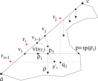
Second, we determine the portion of the bisector $B(r_{j},r_{i+1})$ that appears in $\mbox{$V\!D$}(\overline{cd})$. Since $\rho_{i}$ is horizontal, by Lemma 8, the root $r_{i+1}$ is below $\rho_{i}$. Since $\rho\subset B(r_{j},r_{i})$ with $i>j$, by Invariant (6), $r_{j}$ is to the right of $\rho$. Therefore, the intersection point (denoted by $q_{1}$) of the horizontal line through $r_{i+1}$ and the vertical line through $r_{j}$ is to the southeast of $p_{1}$ (see Fig. 15). We first discuss the portion of $B(r_{j},r_{i+1})$ contained in the rectangle $Rec(p_{1},q_{1})$.

Obviously, $Rec(p_{1},q_{1})$ is contained in the rectangle $Rec(r_{j},r_{i+1})$. Thus, the portion of $B(r_{j},r_{i+1})$ in $Rec(p_{1},q_{1})$ is a portion of the middle segment of $B(r_{j},r_{i+1})$. Further, since $p_{1}$ is the intersection of $\rho_{i}$ and $\rho$, $p_{1}$ is at the intersection of $B(r_{i},r_{i+1})$ and $B(r_{j},r_{i})$. Thus, $p_{1}$ is on $B(r_{j},r_{i+1})$.

We claim that $r_{i+1}$ is to the southwest of $r_{j}$. This can be proved by showing that $r_{i+1}$ is to the southwest of $p_{1}$ and $p_{1}$ is to the southwest of $r_{j}$. Indeed, since $r_{i+1}$ is below $\rho_{i}$ and $\overline{cd}$ is positive-sloped, $p_{1}$ must be to the right of $r_{i+1}$, which also implies that $r_{i+1}$ is to the southwest of $p_{1}$. Similarly, we can show that $p_{1}$ is to the southwest of $r_{j}$.

Because $r_{i+1}$ is to the southwest of $r_{j}$, the middle segment of $B(r_{j},r_{i+1})$ is $-1$-sloped. Denote by $B_{M}^{\prime}(r_{j},r_{i+1})$ the portion of $B(r_{j},r_{i+1})$ contained in $Rec(p_{1},q_{1})$. Based on the above analysis, $B_{M}^{\prime}(r_{j},r_{i+1})$ is a $-1$-sloped line segment with an endpoint at $p_{1}$ and the other endpoint on one of the two edges of $Rec(p_{1},q_{1})$ incident to $q_{1}$ (see Fig. 15). Below we prove that $B_{M}^{\prime}(r_{j},r_{i+1})\cap bay(\overline{cd})$ (i.e., the portion of $B_{M}^{\prime}(r_{j},r_{i+1})$ contained in $bay(\overline{cd})$) appears in $\mbox{$V\!D$}(bay(\overline{cd}))$, implying that we should keep this portion of $B_{M}^{\prime}(r_{j},r_{i+1})$. The proof is similar to that for Lemma 12 and hence we only sketch it here. For convenience, we view $B_{M}^{\prime}(r_{j},r_{i+1})$ as the open segment that does not contain its two endpoints.

It suffices to show that $B_{M}^{\prime}(r_{j},r_{i+1})$ does not intersect any current active ray. Consider any current active ray $\rho^{\prime}$, $\rho^{\prime}\not\in\{\rho,\rho_{i}\}$. Then $\rho^{\prime}$ either is in $S$ or is a ray $\rho_{t}\in\Psi$ with $t>i$.

• If $\rho^{\prime}\in S$, then $\rho^{\prime}$ is vertical by Invariant (1). By Invariant (7), $\rho^{\prime}$ is to the right of the root $r_{j}$, and thus to the right of the rectangle $Rec(p_{1},q_{1})$. Hence, $\rho_{t}$ does not intersect $B_{M}^{\prime}(r_{j},r_{i+1})$ since $B_{M}^{\prime}(r_{j},r_{i+1})$ is strictly inside $Rec(p_{1},q_{1})$.

• If $\rho^{\prime}=\rho_{t}\in\Psi$ with $t>i$, then there are two subcases.

  If $\rho_{t}$ is horizontal, then by Lemma 11, $\rho_{t}$ is below $r_{i+1}$, and is thus below the rectangle $Rec(p_{1},q_{1})$. Hence, $\rho_{t}$ does not intersect $B_{M}^{\prime}(r_{j},r_{i+1})$.

  If $\rho_{t}$ is vertical, then by Lemma 10, the origin $or(\rho_{i})$ is to the northeast of $or(\rho_{t})$. Clearly, $or(\rho_{i})$ is to the left of $Rec(p_{1},q_{1})$ and thus $or(\rho_{t})$ is to the left of $Rec(p_{1},q_{1})$. Since $\rho_{t}$ is vertical, $\rho_{t}$ is also to the left of $Rec(p_{1},q_{1})$. Hence, $\rho_{t}$ does not intersect $B_{M}^{\prime}(r_{j},r_{i+1})$.

The above argument shows that all active rays cannot intersect $B_{M}^{\prime}(r_{j},r_{i+1})$. Hence, the portion of $B_{M}^{\prime}(r_{j},r_{i+1})$ contained in $bay(\overline{cd})$ must appear in $\mbox{$V\!D$}(bay(\overline{cd}))$.

Then, we compute $B_{M}^{\prime}(r_{j},r_{i+1})$ in $O(1)$ time, and let $B_{M}^{\prime}(r_{j},r_{i+1})=\overline{p_{1}p_{1}^{\prime}}$ (see Fig. 15). Note that $p_{1}^{\prime}$ is either on the right edge or the bottom edge of $Rec(p_{1},q_{1})$.

However, $\overline{p_{1}p_{1}^{\prime}}$ may intersect $\partial$. To determine whether such intersection occurs, we move among the trapezoids in the horizontal visibility map $\mbox{$H\!M$}(bay(\overline{cd}))$ from the endpoint $p_{1}$ of $B_{M}^{\prime}(r_{j},r_{i+1})$ along the segment $\overline{p_{1}p_{1}^{\prime}}$, as follows.

Note that the portion of the ray $\rho_{i}$ between its origin $or(\rho_{i})$ and its target point $p=tp(\rho_{i})$ is contained in a single trapezoid of $\mbox{$H\!M$}(bay(\overline{cd}))$, i.e., the trapezoid containing $or(\rho_{i})$, which is already known according to Invariant (14). Further, this trapezoid is the one that contains $p_{1}$ since $p_{1}\in\overline{or(\rho_{i})p}$. Starting at $p_{1}$ in this trapezoid, we move along the segment $\overline{p_{1}p_{1}^{\prime}}$, and enter/exit trapezoids in $\mbox{$H\!M$}(bay(\overline{cd}))$ one after another, until we encounter either $p_{1}^{\prime}$ or an edge of $\partial$ for the first time. In this way, we can determine whether $\overline{p_{1}p_{1}^{\prime}}$ intersects $\partial$. Further, if $\overline{p_{1}p_{1}^{\prime}}$ intersects $\partial$, then the first such intersection point, denoted by $z$, is also found in this moving process; if $B_{M}^{\prime}(r_{j},r_{i+1})$ does not intersect $\partial$, then the trapezoid of $\mbox{$H\!M$}(bay(\overline{cd}))$ containing the point $p_{1}^{\prime}$ is determined. It is easy to see that the running time of the above moving procedure is proportional to the number of trapezoids in $\mbox{$H\!M$}(bay(\overline{cd}))$ that we visit when moving along $\overline{p_{1}p_{1}^{\prime}}$. We will analyze the total running time of the moving process in a global manner later.

Depending on whether $B_{M}^{\prime}(r_{j},r_{i+1})$ ($=\overline{p_{1}p_{1}^{\prime}}$) intersects $\partial$, there are two cases to consider.

Figure 16: Illustrating an example that $B^{\prime}_{M}(r_{j},r_{i+1})$ ($=\overline{p_{1}p_{1}^{\prime}}$) intersects $\partial$ (first at $z$).

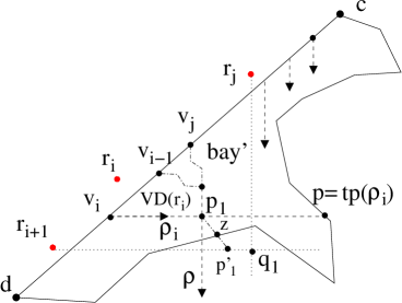
If $B_{M}^{\prime}(r_{j},r_{i+1})$ intersects $\partial$, then we have found the first intersection point $z$ of $B_{M}^{\prime}(r_{j},r_{i+1})$ and $\partial$ (see Fig. 16). Note that $z$ must be after $p$ on $\partial$. Also, note that the Voronoi region $\mbox{$V\!D$}(r_{i})$ has been computed and set as inactive, and thus $p_{1}$ lies on the boundary of the current active region of $bay(\overline{cd})$ (see Fig. 16). Similarly as before, the line segment $\overline{p_{1}z}$ divides the current active region of $bay(\overline{cd})$ into two simple polygons; one of them, say $bay^{\prime}$, contains the point $p$. Then, the Voronoi regions of the roots that define the rays in $S$ form a decomposition of $bay^{\prime}$, and we use a procedure similar to the splitting procedure discussed earlier to compute this decomposition of $bay^{\prime}$, i.e., by considering the rays in $S$ from bottom to top. However, it is possible that the target points of some rays in $S$ have not been computed yet. Recall that all target points of the rays in $S$ before $p$ ($=tp(\rho_{i})$) have been computed. But, if the target point of a ray in $S$ is on $\partial(p,z)$, then it is not yet known. To compute these target points, we simply scan $\partial(p,z)$ from $p$ to $z$. Again, by Invariant (9), the vertical rays in $S$ are target-sorted. Hence this computation can be done in linear time in terms of the number of edges of $\partial(p,z)$ and the number of target points found during this process. In addition, we set the region $bay^{\prime}$ and all rays in $S$ as inactive, and pop all rays out of $S$ ($S$ becomes empty). Finally, we move the reference point $p^{*}$ to $z$, and continue with the next ray $\rho_{i+1}$. Again, since $S$ is empty, similar to the analysis for the subcase 2(a) when $S$ is empty, all invariants of the algorithm hold. We omit the details of the proof.

If $B_{M}^{\prime}(r_{j},r_{i+1})$ ($=\overline{p_{1}p_{1}^{\prime}}$) does not intersect $\partial$ (see Fig. 17), then as shown above, $B_{M}^{\prime}(r_{j},r_{i+1})$ appears entirely in $\mbox{$S\!P\!M$}(\mathcal{F})$ since it is contained inside $bay(\overline{cd})$. Again, the point $p_{1}^{\prime}$ is on either the right edge or the bottom edge of $Rec(p_{1},q_{1})$ (two cases). We discuss these two cases below. Recall that the trapezoid of $\mbox{$H\!M$}(bay(\overline{cd}))$ that contains $p_{1}^{\prime}$ has been computed. Recall that the ray at the top of $S$ is $\rho$, lying on $B(r_{j},r_{i})$ with $i>j$.

We first discuss the case when $p_{1}^{\prime}$ is on the bottom edge of $Rec(p_{1},q_{1})$ (see Fig. 17). Let $\rho_{i}^{*}$ be the vertical ray originating at $p_{1}^{\prime}$ and going south, which is on $B(r_{j},r_{i+1})$ by Observation 2. We pop $\rho$ out of $S$ and push $\rho_{i}^{*}$ onto the top of $S$, and set $\rho$ as inactive and $\rho_{i}^{*}$ as active. We move $p^{*}$ to $p$ ($=tp(\rho_{i})$). We then continue to consider the next ray $\rho_{i+1}\in\Psi$. Lemma 17 below shows that all invariants of the algorithm hold.

Figure 17: Illustrating an example that the point $p_{1}^{\prime}$ ($=or(\rho_{i}^{*})$) is on the bottom edge of $Rec(p_{1},q_{1})$.

Lemma 17

At the moment right before the next ray $\rho_{i+1}$ is considered, all invariants of the algorithm hold.

Proof: Let $\xi$ be the moment right before the next ray $\rho_{i+1}$ is considered, and $\xi^{\prime}$ be the moment right before the ray $\rho_{i}$ is considered. Thus, the change to $S$ from the time $\xi^{\prime}$ to $\xi$ is that $\rho$ is popped out and $\rho_{i}^{*}$ is pushed in. Recall that at the moment $\xi^{\prime}$, all invariants of the algorithm hold. Our goal is to prove that all invariants still hold at the moment $\xi$. We assume that $S$ has at least two rays at the moment $\xi$ (otherwise, all invariants related to any other rays in $S$ than $\rho^{*}_{i}$ hold trivially). Let $\rho^{\prime}$ be the second ray from the top of $S$ (i.e., right below $\rho_{i}^{*}$ in $S$) at the moment $\xi$. Then $\rho^{\prime}$ is also the second ray from the top of $S$ at the moment $\xi^{\prime}$ (i.e., right below $\rho$ in $S$). See Fig. 17 for an example.

Invariant (1) simply follows since $\rho_{i}^{*}$ is vertically going south.

For Invariant (2), it suffices to show that $or(\rho^{*}_{i})$ is to the southwest of $or(\rho^{\prime})$. At the moment $\xi^{\prime}$, since the ray $\rho$ at the top of $S$ is on $B(r_{j},r_{i})$ with $i>j$, by Invariant (6), $r_{j}$ is to the left of $or(\rho^{\prime})$. Since $or(\rho^{*}_{i})\in Rec(r_{j},r_{i+1})$ is to the left of $r_{j}$, we obtain that $or(\rho_{i}^{*})$ is to the left of $or(\rho^{\prime})$. Further, at the moment $\xi^{\prime}$, by Invariant (2), $or(\rho)$ is to the southwest of $or(\rho^{\prime})$. Since $or(\rho_{i}^{*})$ is below $or(\rho)$, $or(\rho_{i}^{*})$ is below $or(\rho^{\prime})$. Since $or(\rho_{i}^{*})$ is both below and to the left of $or(\rho^{\prime})$, we obtain that $or(\rho_{i}^{*})$ is to the southwest of $or(\rho^{\prime})$. Invariant (2) thus follows.

For Invariant (3), we need to show that $or(\rho_{i+1})$ is to the southwest of $or(\rho_{i}^{*})$. By Lemma 10, $or(\rho_{i+1})$ is to the southwest of $or(\rho_{i})$. Since $or(\rho_{i}^{*})$ is to the right of $or(\rho_{i})$, $or(\rho_{i}^{*})$ is also to the right of $or(\rho_{i+1})$. By Lemma 8(3), $or(\rho_{i+1})$ is below $r_{i+1}$. Hence, $or(\rho_{i+1})$ is below the rectangle $Rec(p_{1},q_{1})$ and thus below $or(\rho_{i}^{*})$. Since $or(\rho_{i+1})$ is both below and to the left of $or(\rho_{i}^{*})$, we obtain that $or(\rho_{i+1})$ is to the southwest of $or(\rho_{i}^{*})$. Thus, Invariant (3) follows.

Invariant (4) simply follows since $\rho_{i}^{*}\subset B(r_{j},r_{i+1})$ and $\rho_{i+1}\subset B(r_{i+1},r_{i+2})$.

For Invariant (5), we need to consider both $\rho_{i}^{*}$ and $\rho_{i+1}$. For $\rho_{i}^{*}$, since $\rho_{i}^{*}\subset B(r_{j},r_{i+1})$, we need to show that the boundary portion of the Voronoi region $\mbox{$V\!D$}(r_{i+1})$ (resp., $\mbox{$V\!D$}(r_{j})$) from $v_{i}$ (resp., $v_{j}$) to $or(\rho_{i}^{*})$ has been computed. For this, recall that the boundary portion of $\mbox{$V\!D$}(r_{i+1})$ between $v_{i}$ and $p_{1}$ is a common boundary of $\mbox{$V\!D$}(r_{i+1})$ and $\mbox{$V\!D$}(r_{i})$, which has been computed. We denote this boundary portion by $\alpha$. Also, the boundary portion of $\mbox{$V\!D$}(r_{j})$ between $v_{j}$ and $p_{1}$ has been computed; we denote this boundary portion by $\beta$. Further, after we find the point $p^{\prime}_{1}$, the line segment $\overline{p_{1}p_{1}^{\prime}}$ has also been obtained. Since $\overline{p_{1}p_{1}^{\prime}}$ appears entirely in $\mbox{$S\!P\!M$}(\mathcal{F})$, the boundary portion of $\mbox{$V\!D$}(r_{i+1})$ between $v_{i}$ and $or(\rho_{i}^{*})$ ($=p_{1}^{\prime}$) is the concatenation of $\alpha$ and $\overline{p_{1}p_{1}^{\prime}}$, which has been computed. Similarly, the boundary portion of $\mbox{$V\!D$}(r_{j})$ between $v_{j}$ and $or(\rho_{i}^{*})$ is the concatenation of $\beta$ and $\overline{p_{1}p_{1}^{\prime}}$, which has been computed too. Thus, the case for $\rho_{i}^{*}$ holds.

For the ray $\rho_{i+1}$, which is the ray to be considered next by the algorithm, we need to show that the boundary portion of the Voronoi region $\mbox{$V\!D$}(r_{i+1})$ from $v_{i+1}$ to $or(\rho_{i+1})$, which is also the boundary portion of the Voronoi region $\mbox{$V\!D$}(r_{i+2})$ from $v_{i+1}$ to $or(\rho_{i+1})$, has been computed. This simply follows from Observation 6.

In summary, Invariant (5) holds.

For Invariant (6), it suffices to show that $or(\rho_{i}^{*})$ is to the left of $r_{j}$ and to the right of $r_{i+1}$. Recall that $or(\rho_{i}^{*})$ is on the rectangle $Rec(p_{1},q_{1})$, $q_{1}$ is to the southeast of $p_{1}$, and $q_{1}$ is the intersection of the vertical line through $r_{j}$ and the horizontal line through $r_{i+1}$. As shown above, $r_{i+1}$ is to the left of $p_{1}$. Since $or(\rho_{i}^{*})$ is to the right of $p_{1}$, $or(\rho_{i}^{*})$ is to the right of $r_{i+1}$. Since $Rec(p_{1},q_{1})$ is to the left of $r_{j}$, $or(\rho_{i}^{*})$ is to the left of $r_{j}$. Invariant (6) thus holds.

For Invariant (7), we need to show that $r_{j}$ is to the left of all rays in $S\setminus\{\rho_{i}^{*}\}$. At the moment $\xi^{\prime}$, the ray $\rho\subset B(r_{j},r_{i})$ is at the top of $S$ with $i>j$; thus by Invariant (7), $r_{j}$ is to the left of all rays in $S\setminus\{\rho\}$. Since $S\setminus\{\rho\}=S\setminus\{\rho_{i}^{*}\}$, Invariant (7) still holds at the moment $\xi$.

For Invariant (8), recall that $\rho^{\prime}$ is the second ray from the top of $S$ at both the moments $\xi$ and $\xi^{\prime}$. We assume $\rho^{\prime}$ lying on $B(r_{t},r_{t^{\prime}})$ with $t^{\prime}>t$. To prove Invariant (8) held at $\xi$, it suffices to show $t^{\prime}=j$ since $\rho_{i}^{*}\subset B(r_{j},r_{i+1})$. At the moment $\xi^{\prime}$, since $\rho\subset B(r_{j},r_{i})$ is the ray at the top of $S$, by Invariant (8), we have $j=t^{\prime}$. Thus, Invariant (8) still holds at the moment $\xi$.

For Invariant (9), it suffices to show that $tp(\rho_{i}^{*})$ is after $tp(\rho^{\prime})$ on $\partial$. Intuitively this is true due to the following facts: There is a path inside $bay(\overline{cd})$ from $v_{i}$ to $or(\rho_{i}^{*})$ (i.e., the concatenation of $\overline{v_{i}or(\rho_{i})}$, $\overline{or(\rho_{i})p_{1}}$, and $\overline{p_{1}p_{1}^{\prime}}$), and both $\rho_{i}^{*}$ and $\rho^{\prime}$ are vertical, and $\rho_{i}^{*}$ is to the left of $\rho^{\prime}$. A detailed analysis is given below.

First, it is easy to see that $tp(\rho_{i}^{*})$ must be after the point $p$ ($=tp(\rho_{i})$). The target point $tp(\rho^{\prime})$ may be after $p$ or before $p$. If $tp(\rho^{\prime})$ is before $p$, then we are done. Thus, we consider the case of $tp(\rho^{\prime})$ being after $p$. By Invariant (2) (at the moment $\xi$) proved above, $or(\rho^{\prime})$ is to the northeast of $or(\rho^{*}_{i})$. Thus, the ray $\rho^{\prime}$ must cross $\rho_{i}$ before it hits $\partial$ at $tp(\rho^{\prime})$; in other words, the two line segments $\overline{or(\rho^{\prime})tp(\rho^{\prime})}$ and $\overline{or(\rho_{i})tp(\rho_{i})}$ intersect inside $bay(\overline{cd})$. Further, since $\rho^{\prime}$ is to the right of $\rho^{*}_{i}$ and $p_{1}$ is to the left of $\rho_{i}^{*}$, the intersection point of $\overline{or(\rho^{\prime})tp(\rho^{\prime})}$ and $\overline{or(\rho_{i})tp(\rho_{i})}$ is on $\overline{p_{1}tp(\rho_{i})}$.

Recall that $\overline{v_{i}or(\rho_{i})}$ is either a single point or a line segment that is in $\mbox{$V\!D$}(bay(\overline{cd}))$ and does not intersect $\partial$. Consider the region in $bay(\overline{cd})$ bounded by $\overline{v_{i}or(\rho_{i})}$, $\overline{or(\rho_{i})p}$, and $\partial(p,d)$, which we denote by $Z$. It is easy to see that $Z$ is a simple polygon. Let $\alpha$ be the concatenation of $\overline{p_{1}p^{\prime}_{1}}$ and $\overline{p_{1}^{\prime}tp(p_{i}^{*})}$. Note that $\alpha$ is entirely inside $Z$ except that its two endpoints are on the boundary of $Z$, i.e., $p_{1}\in\overline{or(\rho_{i})p}$ and $tp(p_{i}^{*})\in\partial(p,d)$. Thus, $\alpha$ divides $Z$ into two simple polygons; one of them contains $\overline{p_{1}p}$ as an edge, which is denoted by $Z^{\prime}$. Since the intersection of $\overline{or(\rho^{\prime})tp(\rho^{\prime})}$ and $\overline{or(\rho_{i})tp(\rho_{i})}$ is on $\overline{p_{1}tp(\rho_{i})}$, the ray $\rho^{\prime}$ intersects $Z^{\prime}$. By Invariant (7) (at the moment $\xi$) proved above, the root $r_{j}$ is to the left of $\rho^{\prime}$. Thus, $\rho^{\prime}$ cannot intersect the curve $\alpha$. Hence, the target point $tp(\rho^{\prime})$ must be on the boundary of $Z^{\prime}\cap\partial(p,d)$, which is on $\partial(p,tp(\rho_{i}^{*}))$. Thus, $tp(\rho_{i}^{*})$ is after $tp(\rho^{\prime})$, and Invariant (9) follows.

For Invariant (10), we need to show that if $\rho_{i+1}$ is vertical, then the target point $tp(\rho_{i+1})$ is after $tp(\rho_{i}^{*})$ on $\partial$. By Invariant (3) (at the moment $\xi$) proved above, $or(\rho_{i+1})$ is to the southwest of $or(\rho_{i}^{*})$. Let $Z$ be the simple polygonal region in $bay(\overline{cd})$ bounded by $\overline{v_{i}or(\rho_{i})}$, $\overline{or(\rho_{i})p_{1}}$, $\overline{p_{1}p_{1}^{\prime}}$, $\overline{p^{\prime}_{1}tp(\rho_{i}^{*})}$, $\partial(tp(\rho_{i}^{*}),d)$, and $\overline{dv_{i}}$. Regardless of whether $or(\rho_{i+1})=v_{i+1}$, the origin $or(\rho_{i+1})$ of $\rho_{i+1}$ is in $Z$ since $or(\rho_{i+1})$ is to the southwest of $or(\rho_{i}^{*})=p_{1}^{\prime}$. Further, since both $\rho^{*}_{i}$ and $\rho_{i+1}$ are vertical, $tp(\rho_{i+1})$ must be on $\partial(tp(\rho_{i}^{*}),d)$. Invariant (10) thus follows.

For Invariant (11), it suffices to show that $tp(\rho_{i}^{*})$ is after $p^{*}$ since $tp(\rho_{i}^{*})$ has not been computed. Since $tp(\rho_{i}^{*})$ is after $p=tp(\rho_{i})$ ($=p^{*}$), Invariant (11) simply follows.

For Invariant (12), we need to show that the target point $tp(\rho_{i+1})$ is after $p^{*}$ ($=p=tp(\rho_{i})$). Let $Z$ be the simple polygonal region in $bay(\overline{cd})$ bounded by $\overline{v_{i}or(\rho_{i})}$, $\overline{or(\rho_{i})p}$, $\partial(p,d)$, and $\overline{dv_{i}}$. Clearly, $or(\rho_{i+1})$ is in $Z$. Further, since $or(\rho_{i+1})$ is to the southwest of $or(\rho_{i})$, regardless of whether $\rho_{i+1}$ is vertical or horizontal, $tp(\rho_{i+1})$ must be on $\partial(p^{*},d)$. Thus, Invariant (12) holds.

For Invariant (13), suppose $l$ is the smallest index with $l>i$ such that $\rho_{l}\in\Psi$ and $\rho_{l}$ is horizontal. We need to prove that $tp(\rho_{l})$ is after $p^{*}$ ($=p=tp(\rho_{i})$). Consider the simple polygon $Z$ defined above for proving Invariant (12). Since $\rho_{l}$ is horizontal, by Lemma 11, $\rho_{l}$ is below $r_{i+1}$. Thus, it is easy to see that $or(\rho_{l})$ is in $Z$ and $tp(\rho_{l})$ is on $\partial(p^{*},d)$. Hence, $tp(\rho_{l})$ is after $p^{*}$, and Invariant (13) holds.

For Invariant (14), we need to show that the trapezoid of $\mbox{$H\!M$}(bay(\overline{cd}))$ that contains $or(\rho_{i+1})$ is known, which is true by Observation 6.

We conclude that all invariants of the algorithm still hold at the moment $\xi$. $\Box$

For the purpose of discussing the analysis of the running time of our algorithm later, we call the ray $\rho_{i}^{*}$ the termination vertical ray of the (horizontal) ray $\rho_{i}$.

We have finished the discussion for the case when $p_{1}^{\prime}$ is on the bottom edge of $Rec(p_{1},q_{1})$.

We then discuss the case when the point $p_{1}^{\prime}$ is on the right edge of $Rec(p_{1},q_{1})$ (see Fig. 18). Denote by $\rho_{i1}$ the horizontal ray originating at $p^{\prime}_{1}$ and going east, which is on $B(r_{j},r_{i+1})$ by Observation 2. Then, we pop $\rho$ out of $S$ and set $\rho$ as inactive. Also, we set $\rho_{i1}$ as active and move the reference point $p^{*}$ to $p$ ($=tp(\rho_{i})$). Finally, we let $\rho_{i1}$ be the next ray to be considered by the algorithm (note that $\rho_{i1}$ is not in $\Psi$). Lemma 18 below shows that all invariants of the algorithm hold. Recall that the trapezoid of $\mbox{$H\!M$}(bay(\overline{cd}))$ that contains $p_{1}^{\prime}$ has been computed.

Figure 18: Illustrating an example that the point $p_{1}^{\prime}$ ($=or(\rho_{i1})$) is on the right edge of $Rec(p_{1},q_{1})$.

Lemma 18

At the moment right before the next ray $\rho_{i1}$ is considered, all invariants of the algorithm hold.

Proof: Let $\xi$ be the moment right before the next ray $\rho_{i1}$ is considered, and $\xi^{\prime}$ be the moment right before the ray $\rho_{i}$ is considered. Thus, the only change to $S$ from the time $\xi^{\prime}$ to $\xi$ is that $\rho$ is popped out. At the moment $\xi^{\prime}$, all invariants of the algorithm hold. Our goal is to prove that all invariants still hold at the moment $\xi$. We assume $S\not=\emptyset$ at the moment $\xi$ (otherwise, all invariants related to any rays in $S$ hold trivially). Let $\rho^{\prime}$ be the ray at the top of $S$ at the moment $\xi$. Then $\rho^{\prime}$ is the second ray from the top of $S$ (i.e., right below the ray $\rho$ in $S$) at the moment $\xi^{\prime}$. Refer to Fig. 18 for an example.

Invariants (1) and (2) simply hold.

For Invariant (3), we need to show that $or(\rho_{i1})$ is to the southwest of $or(\rho^{\prime})$. By Invariant (2) at the moment $\xi^{\prime}$, $or(\rho)$ of the ray $\rho$ at the top of $S$ is to the southwest of $or(\rho^{\prime})$. Since $or(\rho_{i1})=p_{1}^{\prime}$ is below $or(\rho)$, $or(\rho_{i1})$ is below $or(\rho^{\prime})$. Also, by Invariant (7) at the moment $\xi^{\prime}$, since the top ray $\rho$ in $S$ is on $B(r_{j},r_{i})$ (with $i>j$), $r_{j}$ is to the left of $\rho^{\prime}$ (which is vertical). Since $p_{1}^{\prime}$ is on the vertical line through $r_{j}$, $p_{1}^{\prime}=or(\rho_{i1})$ is to the left of $or(\rho^{\prime})$. Hence, $or(\rho_{i1})$ is to the southwest of $or(\rho^{\prime})$, and Invariant (3) follows.

For Invariant (4), suppose $\rho^{\prime}$ is on $B(r_{t},r_{t^{\prime}})$ with $t^{\prime}>t$; we need to show $j=t^{\prime}$ since $\rho_{i1}\subset B(r_{j},r_{i+1})$ is the next ray to be considered by the algorithm. At the moment $\xi^{\prime}$, $\rho\subset B(r_{j},r_{i})$ (with $i>j$) is at the top of $S$ and $\rho^{\prime}$ is the second ray from the top of $S$; thus, by Invariant (8) at the moment $\xi^{\prime}$, $j=t^{\prime}$. Invariant (4) hence follows.

For Invariant (5), since no new ray is pushed onto $S$, we only need to consider the ray $\rho_{i1}$. The proof is the same as that for Invariant (5) (for the ray $\rho_{i}^{*}$) in the proof of Lemma 17, and we omit it.

Invariants (6), (7), (8), (9), and (11) trivially hold since no new ray is pushed into $S$.

Invariant (10) simply follows since $\rho_{i1}$ is the next ray to be considered by the algorithm and $\rho_{i1}$ is not vertical.

For Invariant (12), we need to show that the target point $tp(\rho_{i1})$ is after $p^{*}$ ($=p=tp(\rho_{i})$). Consider the simple polygonal region $Z$ in $bay(\overline{cd})$ bounded by $\overline{v_{i}or(\rho_{i})}$, $\overline{or(\rho_{i})p}$, $\partial(p,d)$, and $\overline{dv_{i}}$. It is easy to see that $or(\rho_{i1})$ is in $Z$ and $tp(\rho_{i1})$ is on $\partial(p^{*},d)$. Thus, $tp(\rho_{i1})$ is after $p^{*}$.

For Invariant (13), suppose $l$ is the smallest index with $l>i$ such that $\rho_{l}\in\Psi$ and $\rho_{l}$ is horizontal. We need to prove that $tp(\rho_{l})$ is after $p^{*}$ ($=p=tp(\rho_{i})$). Consider the simple polygon $Z$ defined above for proving Invariant (12). Since $\rho_{l}$ is horizontal, by Lemma 11, $\rho_{l}$ is below $r_{i+1}$. Thus, it is easy to see that $or(\rho_{l})$ is in $Z$ and $tp(\rho_{l})$ is on $\partial(p^{*},d)$. Hence, $tp(\rho_{l})$ is after $p^{*}$, and Invariant (13) holds.

For Invariant (14), recall that the trapezoid of $\mbox{$H\!M$}(bay(\overline{cd}))$ that contains $p_{1}^{\prime}$ ($=or(\rho_{i1})$) has been computed, and thus Invariant (14) holds.

We conclude that all invariants of the algorithm hold at the moment $\xi$. $\Box$

For analysis, we refer to the ray $\rho_{i1}$ as a successor horizontal ray of the (horizontal) ray $\rho_{i}$.

This finished the discussion for the case when $p_{1}^{\prime}$ is on the right edge of $Rec(p_{1},q_{1})$.

Again, $\rho_{i1}$ is the next ray to be considered by the algorithm. Although our earlier discussion on the algorithm processing the next ray is mostly on processing a ray $\rho_{i}\in\Psi$, the processing for $\rho_{i1}$ ($\not\in\Psi$) is the same, and the proof for all invariants is also very similar. In particular, there may also be a termination vertical ray or a successor horizontal ray generated at the end of processing $\rho_{i1}$, which we still refer to as a termination vertical ray or a successor horizontal ray of $\rho_{i}$. It is easy to see that a horizontal ray $\rho_{i}$ may lead to multiple successor horizontal rays but at most one termination vertical ray, i.e., a successor horizontal ray may generate another successor horizontal ray (e.g., see Fig. 19), but a termination vertical ray does not generate another ray.

One might be curious about why the roles of horizontal rays and vertical rays are quite different in our above algorithm, while the $L_{1}$ metric does not prefer one of these two directions over the other. The asymmetric roles of these two directions are related to the order of $\rho_{1},\rho_{2},\ldots,\rho_{k-1}$ in which we process these rays. If one uses a reversed order (i.e., $\rho_{k-1},\rho_{k-2},\ldots,\rho_{1}$) in the processing, then the roles of these two types of rays will be reversed.

For the purpose of analyzing the running time of the algorithm later, we discuss more details related to the successor horizontal rays of a horizontal ray $\rho_{i}\in\Psi$. We process the first successor horizontal ray $\rho_{i1}$ of $\rho_{i}$ in the same way as $\rho_{i}$. After $\rho_{i1}$ is processed, we may obtain another successor horizontal ray $\rho_{i2}$. In general, assume all successor horizontal rays we obtain for $\rho_{i}$ are $\rho_{i1},\rho_{i2},\ldots,\rho_{it}$, ordered by the time when they are produced (see Fig. 19). Then, after the last ray $\rho_{it}$ is processed, we may or may not obtain the termination vertical ray $\rho_{i}^{*}$. For example, when processing $\rho_{it}$, if $S=\emptyset$, then no termination vertical ray is generated. In either case, after $\rho_{it}$ is processed, we continue to consider the next ray $\rho_{i+1}\in\Psi$.

Let $\rho_{i0}=\rho_{i}$. For each $1\leq w\leq t$, we define the points $p_{w+1}$, $q_{w+1}$, and $p^{\prime}_{w+1}$ for the ray $\rho_{iw}$ similarly to the points $p_{1}$, $q_{1}$, and $p^{\prime}_{1}$ for $\rho_{i0}$ (see Fig. 19). Note that when processing $\rho_{it}$, depending on the specific situations, the points $p_{t+1}$, $q_{t+1}$, and $p^{\prime}_{t+1}$ may not exist (e.g., if $S=\emptyset$). In the following, we assume they exist (otherwise, the analysis is actually simpler).

Figure 19: Illustrating the first two successor horizontal rays $\rho_{i1}$ and $\rho_{i2}$ of a horizontal ray $\rho_{i}\in\Psi$.

It is easy to see that for each $1\leq w\leq t$, the ray $\rho_{i,w-1}$ contains the top edge of the rectangle $Rec(p_{w},p_{w}^{\prime})$ and the ray $\rho_{iw}$ touches the bottom edge of $Rec(p_{w},p_{w}^{\prime})$. In addition, the ray $\rho_{it}$ contains the top edge of $Rec(p_{t+1},p_{t+1}^{\prime})$. In other words, $\rho_{i0}$ ($=\rho_{i}$), $Rec(p_{1},p_{1}^{\prime})$, $\rho_{i1}$, $Rec(p_{2},p_{2}^{\prime})$, $\rho_{i2}$, $\ldots$, $Rec(p_{t},p_{t}^{\prime})$, $\rho_{it},Rec(p_{t+1},p_{t+1}^{\prime})$ are ordered from high to low and left to right (see Fig. 19). Thus, no two different rectangles in the sequence above intersect in their interior. Actually, the rectangles $Rec(p_{1},p_{1}^{\prime}),Rec(p_{2},p_{2}^{\prime}),\ldots,Rec(p_{t+1},p_{t+1}^{\prime})$ are ordered from northwest to southeast. Further, all successor horizontal rays and rectangles involved are higher than $r_{i+1}$. To see this fact, note that for each $1\leq w\leq t+1$, the point $p_{w}^{\prime}$ is higher than the point $q_{w}$ and $q_{w}$ is on the horizontal line through $r_{i+1}$ (see Fig. 19). Thus, all these rectangles are contained in the horizontal strip between the horizontal line containing $\rho_{i}$ and the horizontal line through $r_{i+1}$; we denote this strip by $\mbox{$H\!Strip$}(\rho_{i})$. Recall that during our algorithm, the horizontal visibility map $\mbox{$H\!M$}(bay(\overline{cd}))$ is utilized as a guide and we often move among its trapezoids. When computing and processing these successor horizontal rays, we always follow $\mbox{$H\!M$}(bay(\overline{cd}))$, e.g., for each $w=0,1,\ldots,t$, we utilize $\mbox{$H\!M$}(bay(\overline{cd}))$ to compute the target point $tp(\rho_{iw})$ of the ray $\rho_{iw}$, to determine whether $\overline{p_{w+1}p^{\prime}_{w+1}}$ intersects $\partial$, and to find the trapezoid in $\mbox{$H\!M$}(bay(\overline{cd}))$ that contains $p^{\prime}_{w+1}=or(\rho_{i,w+1})$. The discussion above implies that the time for processing all successor horizontal rays of $\rho_{i}$ is proportional to $O(t)$ plus the number of trapezoids in $\mbox{$H\!M$}(bay(\overline{cd}))$ that intersect the horizontal strip $\mbox{$H\!Strip$}(\rho_{i})$ as well as the time for computing the target points of some (vertical) rays in $S$.

In addition, during this process, each of the $t$ successor horizontal rays $\rho_{iw}$ of $\rho_{i}$ corresponds to a ray in $S$ that is popped out. Thus, there are $t$ vertical rays popped out of $S$ for $\rho_{i}$. But, at most one ray, i.e., the termination vertical ray $\rho_{i}^{*}$, is pushed onto $S$ for $\rho_{i}$.

We have finished the description of our algorithm for computing $\mbox{$S\!P\!M$}(bay(\overline{cd}))$, which is summarized by the pseudo-code of Algorithm 1.

5.3.3 The Time Complexity

It remains to analyze the running time of the algorithm. First, we show the following lemma.

Lemma 19

The total number of rays ever contained in the stack $S$ throughout the entire algorithm is at most $k$. Once a ray is popped out of $S$, it will never be pushed back in again.

Proof: When processing each ray $\rho_{i}\in\Psi$, if it is vertical, then we push it onto $S$; if it is horizontal, then as shown above, although there may be multiple successor horizontal rays of $\rho_{i}$, at most one ray, i.e., the termination vertical ray, is put into $S$. Further, according to our algorithm, once a ray in $S$ is popped out, it will never be considered again, and thus never be put into $S$ again. $\Box$

We then discuss the total time for computing the target points for all vertical ray shootings in the entire algorithm. We use a reference point $p^{*}$ on $\partial$ and the vertical visibility map $\mbox{$V\!M$}(bay(\overline{cd}))$ for this purpose. To conduct the vertical ray shootings, because the rays involved are always target-sorted, we simply scan the edges in a portion of $\partial$ between $p^{*}$ and another point $p$ that is after $p^{*}$ on $\partial$. Further, when such a scanning is done, we always move $p^{*}$ to $p$. This implies that any portion of $\partial$ is scanned at most once in the entire algorithm. In addition, the number of all vertical ray shootings is at most $k$. This is because each vertical ray involved is from $S$, and by Lemma 19, the number of rays ever contained in $S$ is at most $k$. Therefore, the total time for computing the target points of all vertical rays in the entire algorithm is $O(n^{\prime}+k)$.

For each ray $\rho_{i}\in\Psi$, if it is vertical, then processing it takes $O(1)$ time, i.e., pushing $\rho_{i}$ onto $S$. If it is horizontal, then assume that $\rho_{i}$ has $t$ successor horizontal rays. We have discussed that, besides the procedure for computing their target points, the time for processing these $t$ successor horizontal rays is proportional to $t$ plus the number of trapezoids in $\mbox{$H\!M$}(bay(\overline{cd}))$ intersecting the horizontal strip $\mbox{$H\!Strip$}(\rho_{i})$. We have also shown that each successor horizontal ray corresponds to a ray in the stack $S$ that is popped out. Since there are at most $k$ rays ever contained in $S$ by Lemma 19, the total number of successor horizontal rays in the entire algorithm is at most $k$. On the other hand, consider two different horizontal rays $\rho_{i}$ and $\rho_{j}$ in $\Psi$. We claim that the two horizontal strips $HStip(\rho_{i})$ and $\mbox{$H\!Strip$}(\rho_{j})$ do not intersect each other in their interior. WLOG, assume $i<j$. Indeed, the strip $\mbox{$H\!Strip$}(\rho_{i})$ is above the horizontal line through the root $r_{i+1}$ and $\mbox{$H\!Strip$}(\rho_{j})$ is below the ray $\rho_{j}$. Since $\rho_{j}$ is horizontal and $j>i$, by Lemma 11, $\rho_{j}$ is below $r_{i+1}$. Our claim thus holds. The above claim implies that, besides the time for computing their target points, the time for processing all successor horizontal rays in the entire algorithm is proportional to the total number of trapezoids in $\mbox{$H\!M$}(bay(\overline{cd}))$ plus $k$, which is $O(n^{\prime}+k)$.

The algorithm performs totally $O(k)$ horizontal ray shootings, for computing the target points of the horizontal rays in $\Psi$ and their successor horizontal rays. Using $\mbox{$H\!M$}(bay(\overline{cd}))$ and based on the fact that we already know (i.e., have computed) the trapezoid of $\mbox{$H\!M$}(bay(\overline{cd}))$ containing the origin of each such horizontal ray, all such horizontal ray shootings can be done in $O(k)$ time.

In summary, the total running time of our algorithm for computing the shortest path map for the bay $bay(\overline{cd})$ is $O(n^{\prime}+m^{\prime})$ (where $m^{\prime}=k-1$ is the number of $\mbox{$S\!P\!M$}(\mathcal{M})$ vertices on $\overline{cd}$). It is easy to see that the size of this SPM is $O(n^{\prime}+m^{\prime})$ (e.g., since the running time is $O(n^{\prime}+m^{\prime})$).

Theorem 5 thus follows.

6 Computing a Shortest Path Map for a Canal

In this section, we show how to compute a shortest path map for a canal, which uses our shortest path map algorithm for a bay in Section 5 as a main procedure.

Consider a canal $canal(x,y)$ with $x$ and $y$ as the corridor path terminals and two gates $\overline{xd}$ and $\overline{yz}$ (e.g., see Fig. 6). There may be $\mbox{$S\!P\!M$}(\mathcal{M})$ vertices on both gates. Let $m_{1}$ (resp., $m_{2}$) be the number of $\mbox{$S\!P\!M$}(\mathcal{M})$ vertices on $\overline{xd}$ (resp., $\overline{yz}$), and $n^{\prime}$ be the number of obstacle vertices of the canal. We show that a shortest path map for the canal can be computed in $O(m_{1}+m_{2}+n^{\prime})$ time. Let $R_{1}$ (resp., $R_{2}$) be the set of roots whose cells in $\mbox{$S\!P\!M$}(\mathcal{M})$ intersect $\overline{xd}$ (resp., $\overline{yz}$).

Recall that we have defined wavefront incoming/outgoing terminals in Section 4.2. Namely, consider the corridor path terminals $x$ and $y$ of $canal(x,y)$. It is possible that $y$ has a shortest path from $s$ via $x$ (i.e., this path contains the corridor path of $canal(x,y)$), in which case there is a “pseudo-cell” in $\mbox{$S\!P\!M$}(\mathcal{M})$ with $x$ as the root and $y$ being the only other point in this “pseudo-cell”; then $x$ is a wavefront incoming terminal and $y$ is the wavefront-outgoing terminal. If neither $y$ has a shortest path from $s$ via $x$ nor $x$ has a shortest path from $s$ via $y$, then both $x$ and $y$ are wavefront-incoming terminals. In this case, there is a point on the corridor path of $canal(x,y)$ that has two shortest paths from $s$, one via $x$ and the other via $y$ (we will use this property to compute an SPM for $canal(x,y)$).

Note that for the two terminals $x$ and $y$, either both of them are wavefront-incoming terminals, or only one of them is an wavefront-incoming terminal and the other is an wavefront-outgoing terminal. Below, we first discuss the former case; the algorithm for the latter case is very similar.

6.1 Both $x$ and $y$ are Wavefront-Incoming Terminals

If both $x$ and $y$ are wavefront-incoming terminals, by the properties of the corridor path, there is a point $p^{*}$ on the corridor path of $canal(x,y)$ such that there exist two shortest paths $\pi_{1}(s,p^{*})$ and $\pi_{2}(s,p^{*})$ from $s$ to $p^{*}$ with $x\in\pi_{1}(s,p^{*})$ and $y\in\pi_{2}(s,p^{*})$. The point $p^{*}$ can be found in $O(n^{\prime})$ time since we know the shortest path distances from $s$ to $x$ and to $y$.

Let $\mbox{$V\!D$}(canal(x,y),R_{1})$ be the (additively) weighted Voronoi diagram of $canal(x,y)$ with respect to the root set $R_{1}$, i.e., we treat $canal(x,y)$ as a bay with the gate $\overline{xd}$. As defined in Section 5, $\mbox{$V\!D$}(canal(x,y),R_{1})$ is the Voronoi decomposition of $canal(x,y)$ with respect to the roots in $R_{1}$. Similarly, let $\mbox{$V\!D$}(canal(x,y),R_{2})$ be the weighted Voronoi diagram of $canal(x,y)$ with respect to the root set $R_{2}$. Using our algorithm in Section 5, $\mbox{$V\!D$}(canal(x,y),R_{1})$ and $\mbox{$V\!D$}(canal(x,y),R_{2})$ can be computed in totally $O(m_{1}+m_{2}+n^{\prime})$ time. Denote by $\mbox{$V\!D$}(canal(x,y),R_{1},R_{2})$ the weighted Voronoi diagram of $canal(x,y)$ with respect to the roots in $R_{1}\cup R_{2}$. As shown in Section 5, after $\mbox{$V\!D$}(canal(x,y),R_{1},R_{2})$ is computed, an SPM on $canal(x,y)$ with the source $s$ can be built in $O(m_{1}+m_{2}+n^{\prime})$ time. Thus, the key is to compute $\mbox{$V\!D$}(canal(x,y),R_{1},R_{2})$. Below, we show how to compute $\mbox{$V\!D$}(canal(x,y),R_{1},R_{2})$ in $O(m_{1}+m_{2}+n^{\prime})$ time with the help of the point $p^{*}$, $\mbox{$V\!D$}(canal(x,y),R_{1})$, and $\mbox{$V\!D$}(canal(x,y),R_{2})$.

To compute $\mbox{$V\!D$}(canal(x,y),R_{1},R_{2})$, our strategy is to find a “dividing curve” in $canal(x,y)$ that divides $canal(x,y)$ into two simple polygons $C_{1}$ and $C_{2}$, such that each point in $C_{1}$ has a shortest path from $s$ via a root in $R_{1}$ and each point in $C_{2}$ has a shortest path from $s$ via a root in $R_{2}$. Further, each point on the dividing curve has two shortest paths from $s$, one path containing a root in $R_{1}$ and the other path containing a root in $R_{2}$. After finding $C_{1}$ and $C_{2}$, we simply apply the algorithm in Section 5 on $C_{1}$ and $R_{1}$ to compute the weighted Voronoi diagram of $C_{1}$ with respect to $R_{1}$, i.e., $\mbox{$V\!D$}(C_{1},R_{1})$. We similarly compute $\mbox{$V\!D$}(C_{2},R_{2})$. Then, $\mbox{$V\!D$}(canal(x,y),R_{1},R_{2})$ consists of $\mbox{$V\!D$}(C_{1},R_{1})$ and $\mbox{$V\!D$}(C_{2},R_{2})$. Thus, our remaining task is to compute a dividing curve in $canal(x,y)$, which we denote by $\gamma$.

Note that the point $p^{*}\in\gamma$. Computing $\gamma$ can be done in $O(n^{\prime}+m_{1}+m_{2})$ time by a procedure similar to the merge procedure of the divide-and-conquer algorithm for computing the Voronoi diagram of a set of points in the plane [34]. The details are given below.

To compute $\gamma$, we start at the point $p^{*}$ and trace $\gamma$ out by traversing some corresponding cells in $\mbox{$V\!D$}(canal(x,y),R_{1})$ and in $\mbox{$V\!D$}(canal(x,y),R_{2})$ simultaneously. Specifically, we first compute a triangulation of $\mbox{$V\!D$}(canal(x,y),R_{1})$, denoted by $Tri_{1}$, and a triangulation of $\mbox{$V\!D$}(canal(x,y),R_{2})$, denoted by $Tri_{2}$ (this can be done in linear time [3] since each cell of $\mbox{$V\!D$}(canal(x,y),R_{1})$ and $\mbox{$V\!D$}(canal(x,y),R_{2})$ is a simple polygon). Since $p^{*}$ is in a triangle (say, $tri_{1}$) of $Tri_{1}$ and is in a triangle (say, $tri_{2}$) of $Tri_{2}$, we find $tri_{1}$ in $Tri_{1}$ and $tri_{2}$ in $Tri_{2}$. From the cell of $\mbox{$V\!D$}(canal(x,y),R_{1})$ (resp., $\mbox{$V\!D$}(canal(x,y),R_{2})$) that contains $tri_{1}$ (resp., $tri_{2}$), we obtain the root $r_{1}$ (resp., $r_{2}$) of that cell. We then move along the bisector $B(r_{1},r_{2})$ inside $canal(x,y)$, starting at $p^{*}$ and going in each of the two directions along $B(r_{1},r_{2})$. As following a line segment or a ray of $B(r_{1},r_{2})$ in a direction, we determine, in $O(1)$ time, which of $tri_{1}$ or $tri_{2}$ that we exit first. As we cross from one triangle $tri$ (say, in $Tri_{1}$) to the next triangle $tri^{\prime}$, we check which of the following cases occurs: (i) The next triangle $tri^{\prime}$ (in $Tri_{1}$) is contained in the same cell of $\mbox{$V\!D$}(canal(x,y),R_{1})$ as that containing $tri$; (ii) $tri^{\prime}$ is contained in a different cell of $\mbox{$V\!D$}(canal(x,y),R_{1})$ than that containing $tri$; (iii) the movement touches the boundary of $canal(x,y)$ (thus $tri^{\prime}$ does not exist). In Case (i), we continue to follow the same bisector (say, $B(r_{1},r_{2})$). In Case (ii), we find the root (say, $r^{\prime}_{1}$) of the next cell of $\mbox{$V\!D$}(canal(x,y),R_{1})$; then we compute a new bisector (say, $B(r^{\prime}_{1},r_{2})$), and our movement continues along $B(r^{\prime}_{1},r_{2})$. In Case (iii), the movement reaches an end of $\gamma$ (on the boundary of $canal(x,y)$). The dividing curve $\gamma$ is the concatenation of the portions of the bisectors thus traversed.

Due to the properties of the cells of $\mbox{$V\!D$}(canal(x,y),R_{1})$ and $\mbox{$V\!D$}(canal(x,y),R_{2})$, our movement above can visit each triangle of $Tri_{1}$ and $Tri_{2}$ at most once, taking $O(1)$ time per triangle visited. Thus, the partition curve $\gamma$ is computed in $O(n^{\prime}+m_{1}+m_{2})$ time.

In summary, in this case, an SPM on $canal(x,y)$ can be computed in $O(n^{\prime}+m_{1}+m_{2})$ time.

6.2 Only One of $x$ and $y$ is a Wavefront-Incoming Terminal

In this case, exactly one of $x$ and $y$ is a wavefront-incoming terminal. The algorithm is similar to that for the former case. The only difference is on how to find a point $p^{*}$ on the dividing curve $\gamma$ because in this case no such a point $p^{*}$ can be on the corridor path of $canal(x,y)$.

WLOG, we assume that $x$ is a wavefront-incoming terminal and $y$ is not. Then each point on the corridor path (including $y$) has a shortest path from $s$ via $x$. Further, the shortest path through $x$ passes $y$ and goes to the outside of $canal(x,y)$, which means that $y$ is the root of a cell $C(y)$ in $\mbox{$S\!P\!M$}(\mathcal{M})$. If the canal gate $\overline{yz}$ is completely contained in the cell $C(y)$, then it is easy to see that $\mbox{$V\!D$}(canal(x,y),R_{1})$ is $\mbox{$V\!D$}(canal(x,y),R_{1},R_{2})$. Otherwise, as in the former case, we need to find a dividing curve $\gamma$ to divide $canal(x,y)$ into two polygons $C_{1}$ and $C_{2}$ such that each point in $C_{1}$ has a shortest path from $s$ via a root in $R_{1}$ and each point in $C_{2}$ has a shortest path from $s$ via a root in $R_{2}$. To obtain $\gamma$, the key is to find a point $p^{*}\in\gamma$. Since the canal gate $\overline{yz}$ is not completely contained in $C(y)$, there must be a point $q$ on $\overline{yz}$ that is on the common boundary of $C(y)$ and another cell $C(r)$ in $\mbox{$S\!P\!M$}(\mathcal{M})$. We claim that $q$ is on $\gamma$. Indeed, note that $r$ is in $R_{2}$. Hence there is a shortest path $\pi_{1}(s,q)$ from $s$ to $q$ that contains $x$, the corridor path in $canal(x,y)$, and the line segment $\overline{yq}$, and there is another shortest path $\pi_{2}(s,q)$ from $s$ to $q$ via the root $r\in R_{2}$. In other words, $q$ has two shortest paths from $s$, one via a root in $R_{1}$ and the other via a root in $R_{2}$. Therefore, $q$ is on the dividing curve $\gamma$. The rest of the algorithm is similar to that for the former case.

In summary, in this case, an SPM on $canal(x,y)$ can also be built in $O(n^{\prime}+m_{1}+m_{2})$ time.

Therefore, a shortest path map SPM on $canal(x,y)$ can be computed in $O(n^{\prime}+m_{1}+m_{2})$ time. Similarly, the size of this SPM is $O(n^{\prime}+m_{1}+m_{2})$.

Theorem 6 thus follows.

7 Applications of Our Shortest Path Algorithms

In this section, we extend our techniques to solve some other problems.

7.1 The $L_{1}$ Geodesic Voronoi Diagram

Given a set $\mathcal{P}$ of $h$ polygonal obstacles of totally $n$ vertices and a set of $m$ point sites, the $L_{1}$-GVD problem aims to construct the $L_{1}$ geodesic Voronoi diagram of for the $m$ point sites. Denote by $G\!V\!D(\mathcal{P})$ the Voronoi diagram that we want to construct.

Mitchell’s algorithm [29, 30] can be modified to compute $G\!V\!D(\mathcal{P})$ in $O((n+m)\log(n+m))$ time. Namely, instead of initiating a wavelet at a single source, the modified algorithm for $G\!V\!D(\mathcal{P})$ initiates a wavelet at each point site. The rest of the algorithm remains the same as before.

We can also extend our $S\!P\!M$ algorithm in a similar way to compute $G\!V\!D(\mathcal{P})$. Generally, since our algorithm makes use of Mitchell’s algorithm [29, 30] as a main procedure when computing the shortest path map $\mbox{$S\!P\!M$}(\mathcal{M})$ for the ocean $\mathcal{M}$, to compute $G\!V\!D(\mathcal{P})$, we can simply replace Mitchell’s algorithm by its modified version for computing $L_{1}$ geodesic Voronoi diagrams. More specifically, our algorithm for computing $G\!V\!D(\mathcal{P})$ has the following steps. (1) Compute a triangulation of the free space, in which the $m$ point sites are treated as $m$ point obstacles. (2) Compute the corridor structure on $\mathcal{P}$ and the $m$ point obstacles that consists of $O(m+h)$ corridors, which partition the plane into a set $\mathcal{P}^{\prime}$ of $O(m+h)$ convex polygons of totally $O(n+m)$ vertices. (3) Compute the core set $core(\mathcal{P}^{\prime})$ for the convex polygons in $\mathcal{P}^{\prime}$. (4) Apply Mitchell’s modified algorithm [29, 30] to compute the $L_{1}$ geodesic Voronoi diagram $G\!V\!D(core(\mathcal{P}^{\prime}))$ on the core set $core(\mathcal{P}^{\prime})$. (5) Based on $G\!V\!D(core(\mathcal{P}^{\prime}))$, compute the $L_{1}$ geodesic Voronoi diagram $G\!V\!D(\mathcal{P}^{\prime})$ on the convex polygon set $\mathcal{P}^{\prime}$. Although we have multiple sources, this step is the same as before (i.e., as in Lemma 5). (6) Based on $G\!V\!D(\mathcal{P}^{\prime})$, compute the Voronoi regions in all bays and canals, as in Sections 5 and 6. Again, the algorithms for this step are as before, i.e., as the algorithms in Sections 5 and 6. We then obtain the final $L_{1}$ geodesic Voronoi diagram $G\!V\!D(\mathcal{P})$.

To analyze the running time, Steps (1), (2), and (3) are the same as before except that the number of obstacles becomes $m+h$. Specifically, the triangulation in Step (1) takes $O(n+(h+m)\log^{1+\epsilon}(h+m))$ time [2]. Steps (2) and (3) together take $O(n+(h+m)\log(h+m))$ time. Step (4) takes $O((m+h)\log(m+h))$ time since the core set $core(\mathcal{P}^{\prime})$ has totally $O(m+h)$ vertices. Steps (5) and (6) are also the same as before, which take linear time, i.e., $O(n+m)$. Therefore, the entire algorithm takes $O(n+(h+m)\log^{1+\epsilon}(h+m))$ time, which is dominated by the time of the triangulation procedure in Step (1).

Theorem 8

The $L_{1}$ geodesic Voronoi diagram of $m$ point sites among a set of $h$ pairwise disjoint polygonal obstacles of totally $n$ vertices in the plane can be computed in $O(n+(h+m)\log^{1+\epsilon}(h+m))$ time (or $O(n+(h+m)\log(h+m))$ time if a triangulation is given).

If the $m$ point sites are all inside a simple polygon, then Theorem 8 leads to the following result.

Corollary 2

The $L_{1}$ geodesic Voronoi diagram of a set of $m$ point sites in a simple polygon can be computed in $O(n+m\log^{1+\epsilon}m)$ time (or $O(n+m\log m)$ time if a triangulation is given).

Note that the currently fastest known G​V​D algorithm for the Euclidean version of the single simple polygon case runs in $O((n+m)\log(n+m))$ time [32].

Remark. Since the given $m$ sites are points, there is an alternative triangulation algorithm that may be faster (than simply applying the algorithm in [2]) in some situations. The algorithm works as follows: (1) Compute the triangulation of the free space without considering the $m$ sites; (2) find the triangles in the triangulation that contain those $m$ sites (e.g., by a point location data structure); (3) triangulate those triangles that contain at least one point site by considering the point sites as obstacles. It is easy to see that this algorithm takes $O(n+m\log n)$ time in the single polygon case and $O(n+h\log^{1+\epsilon}h+m\log n)$ time in the polygonal domain case. Therefore, using this triangulation algorithm, the geodesic Voronoi diagram can be constructed in $O(n+m(\log n+\log m))$ time in the single polygon case and in $O(n+h\log^{1+\epsilon}h+m\log n+(h+m)\log(h+m))$ time in the polygonal domain case.

7.2 Shortest Paths with Fixed Orientations and Approximate Euclidean Shortest Paths

As in [29, 30], our algorithms can be generalized to solving the $C$-oriented shortest path problem [37]. A $C$-oriented path is a polygonal path with each edge parallel to one of a given set $C$ of fixed orientations. A shortest $C$-oriented path between two points is a $C$-oriented path with the minimum Euclidean distance. Rectilinear paths are a special case of this problem with two fixed orientations of $0$ and $\pi/2$. Let $c=|C|$. Mitchell’s algorithm [29, 30] can compute a shortest $C$-oriented path in $O(cn\log n)$ time and $O(cn)$ space among $h$ pairwise disjoint polygons of totally $n$ vertices in the plane. Similarly, our algorithms also work for this problem, as follows.

We first consider the convex case (i.e., all polygons are convex). We compute a core for each convex polygon based on the orientations in $C$. Note that in this case, a core has $O(c)$ vertices. Thus, we obtain a core set of totally $O(ch)$ vertices. We then apply Mitchell’s algorithm for the fixed orientations of $C$ on the core set to compute a shortest path avoiding the cores in $O(c^{2}h\log ch)$ time and $O(c^{2}h)$ space, after which we find a shortest path avoiding the input polygons in additional $O(n)$ time as in Lemma 4. Thus, a shortest path can be found in totally $O(n+c^{2}h\log ch)$ time and $O(n+c^{2}h)$ space. For the general case when the polygons need not be convex, the algorithm scheme is similar to our $L_{1}$ algorithm in Section 4. In summary, we have the following result.

Theorem 9

Given a set $C$ of orientations and a set of $h$ pairwise disjoint polygonal obstacles of totally $n$ vertices in the plane, we can compute a $C$-oriented shortest $s$-$t$ path in the free space in $O(n+h\log^{1+\epsilon}h+c^{2}h\log ch)$ time (or $O(n+c^{2}h\log ch)$ time if a triangulation is given) and $O(n+c^{2}h)$ space, where $c=|C|$.

This also yields an approximation algorithm for computing a Euclidean shortest path between two points among polygonal obstacles. Since the Euclidean metric can be approximated within an accuracy of $O(1/c^{2})$ if we use $c$ equally spaced orientations, as in [29, 30], Theorem 9 leads to an algorithm that computes a path guaranteed to have a length within a factor $(1+\delta)$ of the Euclidean shortest path length, where $c$ is chosen such that $\delta=O(1/c^{2})$.

Corollary 3

A $\delta$-optimal Euclidean shortest path between two points among $h$ pairwise disjoint polygons of totally $n$ vertices in the plane can be computed in $O(n+h\log^{1+\epsilon}h+(1/\delta)h\log\frac{h}{\sqrt{\delta}})$ time (or $O(n+(1/\delta)h\log\frac{h}{\sqrt{\delta}})$ time if a triangulation is given) and $O(n+(1/\delta)h)$ space.

8 Conclusions

We present new algorithms for solving $L_{1}$ shortest path problems in polygonal domains. Our algorithms are optimal if the triangulation for the free space can be done optimally (i.e., $T=O(n+h\log h)$). In fact, our results show that building an $L_{1}$ shortest path map is equivalent to the triangulation in terms of the running time.

Some of our techniques may be helpful on solving the Euclidean version of the problem. For the Euclidean version, as the $L_{1}$ version, a long-standing open problem is to compute a shortest path in $O(n+h\log h)$ time and $O(n)$ space. Hershberger and Suri [19] built an SPM of size $O(n)$ in $O(n\log n)$ time and $O(n\log n)$ space. Recently, Inkulu et al. announced an algorithm that can find an Euclidean shortest path in $O(n+h\log h\log n)$ time [22]; we give an algorithm for the problem that runs in $O(n+h\log^{1+\epsilon}h+k)$ time [8], where $k$ is a parameter sensitive to the input and is bounded by $O(h^{2})$. Note that our algorithm [8] particularly works for obstacles that have curved boundaries. To generalize the techniques given in this paper to the Euclidean version, some difficulty appears. For example, the idea of using cores does not seem to work (e.g., Lemma 4 is not applicable to the Euclidean version). A possible direction for solving the Euclidean version is to first solve the convex case with the performance desired by the open problem. If this is possible, then by generalizing the techniques given in this paper, it is very likely that the general case may also be solved accordingly, and thus the open problem can be settled although we may still have to suffer the $O(n+h\log^{1+\epsilon}h)$ triangulation time.

References

- [1] M.J. Atallah, D.Z. Chen, and H. Wagener. An optimal parallel algorithm for the visibility of a simple polygon from a point. Journal of the ACM, 38(3):516–533, 1991.
- [2] R. Bar-Yehuda and B. Chazelle. Triangulating disjoint Jordan chains. International Journal of Computational Geometry and Applications, 4(4):475–481, 1994.
- [3] B. Chazelle. Triangulating a simple polygon in linear time. Discrete and Computational Geometry, 6:485–524, 1991.
- [4] B. Chazelle, H. Edelsbrunner, M. Grigni, L. Guibas, J. Hershberger, J. Sharir, and J. Snoeyink. Ray shooting in polygons using geodesic triangulations. Algorithmica, 12(1):54–68, 1994.
- [5] B. Chazelle and L. Guibas. Visibility and intersection problems in plane geometry. Discrete Comput. Geom., 4:551–589, 1989.
- [6] D.Z. Chen, K.S. Klenk, and H.-Y.T. Tu. Shortest path queries among weighted obstacles in the rectilinear plane. SIAM Journal on Computing, 29(4):1223–1246, 2000.
- [7] D.Z. Chen and H. Wang. Computing shortest paths amid pseudodisks. In Proc. of the 22nd Annual ACM-SIAM Symposium on Discrete Algorithms (SODA), pages 309–326, 2011.
- [8] D.Z. Chen and H. Wang. Computing shortest paths among curved obstacles in the plane. In arXiv:1103.3911, 2011.
- [9] K. Clarkson. Approximation algorithms for shortest path motion planning. In Proc. of the 19th Annual ACM Symposium on Theory of Computing, pages 56–65, 1987.
- [10] K. Clarkson, S. Kapoor, and P. Vaidya. Rectilinear shortest paths through polygonal obstacles in time. In Proc. of the 3rd Annual Symposium on Computational Geometry, pages 251–257, 1987.
- [11] K. Clarkson, S. Kapoor, and P. Vaidya. Rectilinear shortest paths through polygonal obstacles in time. Manuscript, 1988.
- [12] P.J. de Rezende, D.T. Lee, and Y.F. Wu. Rectilinear shortest paths with rectangular barriers. In Proc. of the 1st Annual Symposium on Computational Geometry, pages 204–213, 1985.
- [13] H. Edelsbrunner, L. Guibas, and J. Stolfi. Optimal point location in a monotone subdivision. SIAM Journal on Computing, 15(2):317–340, 1986.
- [14] S. Fortune. A sweepline algorithm for Voronoi diagrams. Algorithmica, 2:153–174, 1987.
- [15] S.K. Ghosh and D.M. Mount. An output-sensitive algorithm for computing visibility graphs. SIAM Journal on Computing, 20(5):888–910, 1991.
- [16] L. Guibas, J. Hershberger, D. Leven, M. Sharir, and R.E. Tarjan. Linear-time algorithms for visibility and shortest path problems inside triangulated simple polygons. Algorithmica, 2(1-4):209–233, 1987.
- [17] J. Hershberger and J. Snoeyink. Computing minimum length paths of a given homotopy class. Computational Geometry: Theory and Applications, 4(2):63–97, 1994.
- [18] J. Hershberger and S. Suri. A pedestrian approach to ray shooting: Shoot a ray, take a walk. Journal of Algorithms, 18(3):403–431, 1995.
- [19] J. Hershberger and S. Suri. An optimal algorithm for Euclidean shortest paths in the plane. SIAM Journal on Computing, 28(6):2215–2256, 1999.
- [20] S. Hertel and K. Mehlhorn. Fast triangulation of the plane with respect to simple polygons. Information and Control, 64:52–76, 1985.
- [21] R. Inkulu and S. Kapoor. Planar rectilinear shortest path computation using corridors. Computational Geometry: Theory and Applications, 42(9):873–884, 2009.
- [22] R. Inkulu, S. Kapoor, and S.N. Maheshwari. A near optimal algorithm for finding Euclidean shortest path in polygonal domain. In arXiv:1011.6481v1, 2010.
- [23] B. Joe and R.B. Simpson. Corrections to Lee’s visibility polygon algorithm. BIT, 27:458–473, 1987.
- [24] S. Kapoor and S.N. Maheshwari. Efficient algorithms for Euclidean shortest path and visibility problems with polygonal obstacles. In Proc. of 4th Annual ACM Symposium on Computational Geometry, pages 172–182, 1988.
- [25] S. Kapoor, S.N. Maheshwari, and J.S.B. Mitchell. An efficient algorithm for Euclidean shortest paths among polygonal obstacles in the plane. Discrete and Computational Geometry, 18(4):377–383, 1997.
- [26] D. Kirkpatrick. Optimal search in planar subdivisions. SIAM Journal on Computing, 12(1):28–35, 1983.
- [27] R.C. Larson and V.O.K. Li. Finding minimum rectilinear distance paths in the presence of barriers. Networks, 11:285–304, 1981.
- [28] D.T. Lee. Visibility of a simple polygon. Computer Vision, Graphics, and Image Processing, 22(2):1983, 207–221.
- [29] J.S.B. Mitchell. An optimal algorithm for shortest rectilinear paths among obstacles. Abstracts of the 1st Canadian Conference on Computational Geometry, 1989.
- [30] J.S.B. Mitchell. shortest paths among polygonal obstacles in the plane. Algorithmica, 8(1):55–88, 1992.
- [31] J.S.B. Mitchell. Shortest paths among obstacles in the plane. International Journal of Computational Geometry and Applications, 6(3):309–332, 1996.
- [32] E. Papadopoulou and D.T. Lee. A new approach for the geodesic Voronoi diagram of points in a simple polygon and other restricted polygonal domains. Algorithmica, 20:319–352, 1998.
- [33] H. Rohnert. Shortest paths in the plane with convex polygonal obstacles. Information Processing Letters, 23(2):71–76, 1986.
- [34] M.I. Shamos and D. Hoey. Closest-point problems. In Proc. of the 16th Annual Symposium on Foundations of Computer Science, pages 151–162, 1975.
- [35] J.A. Storer and J.H. Reif. Shortest paths in the plane with polygonal obstacles. Journal of the ACM, 41(5):982–1012, 1994.
- [36] P. Widmayer. On graphs preserving rectilinear shortest paths in the presence of obstacles. Annals of Operations Research, 33(7):557–575, 1991.
- [37] P. Widmayer, Y.F. Wu, and C.K. Wong. On some distance problems in fixed orientations. SIAM Journal on Computing, 16(4):728–746, 1987.