The critical line of two-flavor QCD at finite isospin or baryon densities from imaginary chemical potentials
Abstract
We determine the (pseudo)critical lines of QCD with two degenerate staggered fermions at nonzero temperature and quark or isospin density, in the region of imaginary chemical potentials; analytic continuation is then used to prolongate to the region of real chemical potentials. We obtain an accurate determination of the curvatures at zero chemical potential, quantifying the deviation between the case of finite quark and of finite isospin chemical potential. Deviations from a quadratic dependence of the pseudocritical lines on the chemical potential are clearly seen in both cases: we try different extrapolations and, for the case of nonzero isospin chemical potential, confront them with the results of direct Monte Carlo simulations. Finally we find that, as for the finite quark density case, an imaginary isospin chemical potential can strengthen the transition till turning it into strong first order.
pacs:
11.15.Ha, 12.38.Gc, 12.38.AwI Introduction
The determination of the QCD phase diagram in the temperature - quark density plane is becoming increasingly important, due to its impact in cosmology and in the physics of compact stars and of heavy-ion collisions.
The first-principle nonperturbative approach of discretizing QCD on a space-time lattice and performing numerical Monte Carlo simulations is plagued, at nonzero quark chemical potential, by the well-known sign problem: the fermionic determinant is complex and the Monte Carlo sampling becomes unfeasible. An exact solution to the problem is yet not known, but various approximate alternatives have been explored. One possibility is to investigate other models which are free of the sign problem, like two-color QCD or QCD with a finite isospin density son ; kogut ; however in such approach predictivity is plagued by the fact that systematic differences between the model and the original theory are not known a priori.
A positive measure is obtained also when the quark chemical potential is purely imaginary, in this case the idea is to infer the behavior at real chemical potential by analytic continuation. Such approach was first suggested in Ref. Alford:1998sd , while the effectiveness of the method of analytic continuation was pushed forward in Ref. Lombardo:1999cz . Since then, the method has been extensively applied to QCD with staggered muim ; immu_dl ; azcoiti ; chen ; defor06 ; sqgp ; 2im ; cea3 and Wilson quarks Wu:2006su ; NN2011 and tested in QCD-like theories free of the sign problem Hart:2000ef ; giudice ; cea ; cea1 ; conradi ; Shinno:2009jw ; cea2 and in spin models potts3d ; kt .
The idea underlying the method of analytic continuation is very simple: if the dependence of an observable or of the critical line itself on the imaginary quark chemical potential is expressed in terms of an analytic function inside a certain domain, then this analytic function can be prolongated to the largest possible domain, compatible with the presence of singularities, up to the physically relevant region of real chemical potentials.
There are, however, two important limitations to the effectiveness of the method: a practical one, due to the fact that Monte Carlo simulations yield data points (with statistical uncertainties) at fixed values of the imaginary chemical potential and, therefore, analytic continuation passes through the choice of an interpolating function, which may be ambiguous; a principle one, due to the nonanalyticities and the periodicity of the theory with imaginary chemical potential rw , which makes so that the region effectively available for Monte Carlo simulations is limited by the condition Im. The combination of these two drawbacks implies that the region of real chemical potentials where the analytic continuation is expected to be reliable can be estimated as Re.
Apart from analytic continuation, a careful study of the phase diagram in the - Im() plane is important by its own. It may teach us something about the critical properties of QCD also at zero or small real defor06 ; sqgp ; deph2 ; rwep ; rwep_nf3 ; rwep2 ; rwep3 and, at the same time, it can be used to the test the reliability of QCD-like models which are then used to explore real as well kouno ; braun ; sakai ; aarts ; pawlowski ; kouno_2011 ; rafferty ; pagura ; kashiwa ; morita .
An important role is played in this respect by the periodic series of unphysical first order lines, located at Im, , being the number of colors, which characterize the high- region of the - Im() plane (Roberge-Weiss lines). Such lines are connected to the analytic continuation of the physical pseudocritical line by an endpoint which, both for and QCD, is first order (triple point) in the limit of small or high quark masses and second order for intermediate mass values; it has been conjectured that this may be directly related to the nature of the phase transition at zero or small real chemical potential rwep ; rwep_nf3 ; rwep2 ; rwep3 .
In a series of studies by some of us, we have started a detailed investigation aimed at checking the reliability of analytic continuation of the pseudocritical line and at extending its range of applicability, by looking for possible deviations from the simple linear behavior in , , which fitted well with earlier studies muim ; immu_dl . To this purpose, the range of Im values included in numerical simulations was extended with respect to earlier studies, up to reaching the border of the first Roberge-Weiss (RW) sector, statistics was considerably increased and different kind of interpolating functions were considered. In order to validate the different interpolation options, in some cases QCD-like theories were adopted (such as SU(2) or SU(3) with finite isospin density) which, being free of the sign problem, allowed the comparison of extrapolations with the results of Monte Carlo simulations performed directly at real . A detailed summary of such investigation is reported in Section II, the main result emerging from it is that non-linear corrections are not negligible, but an unambiguous extrapolation to real fails for .
In the present study we consider QCD in presence of a quark () or an isospin 111 Notice that, in order to permit a direct comparison with , we define , where and are the and quark chemical potentials, i.e. a factor 2 lower than usual. () chemical potential, whose partition function, in the standard staggered discretization for fermion fields, reads
| (1) |
where the plus/minus sign refers to the quark/isospin chemical potential case, is the lattice gauge action and is the fermion matrix in the standard staggered formulation:
| (2) | |||||
Here and refer to lattice sites, is a unit vector on the lattice, are the staggered phases, is the lattice spacing and is the bare quark mass. We shall consider a bare quark mass , corresponding to a pion mass MeV.
The partition function in Eq. (1) is expressed as a functional
integral with a positive measure, hence suitable for Monte Carlo evaluation,
when is purely imaginary, but also when is real for
alone. Our plan is to perform an extensive investigation
about the location and the nature of the deconfinement transition
for all cases in which Monte Carlo simulations are available.
The specific purposes that we have in mind are the following:
1)
verify the reliability of analytic continuation of the
critical line, , from imaginary to
real
in the case of a finite , where
simulations are available both for imaginary and real .
Apply analytic continuation to the case of a finite ,
also on the basis
of what learned in the case of a finite ;
2)
make a careful comparison between the two theories at finite
or , quantifying systematic
differences for quantities like
the curvature of the pseudocritical line at zero chemical potential;
3)
determine how the nature of the transition changes as a function
of the chemical potentials. In particular, in the case of a finite ,
no critical point is expected on the imaginary side
since the adopted quark mass, , is
slightly above the lower tricritical quark mass determined
for in Ref. rwep2 , hence the endpoint of the RW
line is second order. The situation can be different,
hence potentially more interesting,
in the case of a finite , where the available
range of imaginary values is larger.
Most numerical simulations have been performed on a lattice; different spatial sizes have been taken into account to investigate the critical behavior in a few specific cases. The paper is organized as follows. In Section II we discuss our determination of the critical line and its analytic continuation to real chemical potentials. Section III is dedicated to a systematic comparison between the curvatures of the critical lines at finite and respectively. In Section IV we discuss how the order of the transition changes as a function of the chemical potential. In Section V we summarize our results and draw our conclusions. A partial account of our findings has been reported in Ref. proc_lat11 .
II Analytic continuation of the pseudocritical line
Before presenting results for QCD, it
is worth making a short summary of our previous findings.
1) In SU(2) with staggered fermions and finite quark density
it was found that the analytic continuation of physical observables is
improved if ratios of polynomials (or Padé
approximants Lombardo:2005ks ) are used as interpolating functions cea .
2) In SU(2) with staggered fermions and finite quark
density cea1 ; cea2 and in SU(3) with staggered fermions and
finite isospin density cea2 it was found that the nonlinear terms in
the dependence of the pseudocritical coupling on in general
cannot be neglected and that the extrapolation to real
may be wrong otherwise.
Moreover, the coefficients of a Taylor expansion in
of were found to be all negative,
implying subtle cancellations
of nonlinear terms at
imaginary in the first RW sector,
hence a practical difficulty in the detection of such terms
from simulations at only.
It was realized
that, in general, a 3-parameter fit (e.g. an even polynomial of order
, with the coefficient of the term possibly constrained by
a fit restricted to smaller values) provided a very good
description of the pseudocritical line in all explored cases.
3) In SU(3) with staggered fermions and finite quark
density cea3 deviations in the pseudocritical line from the
linear behavior in for larger absolute values of were clearly
seen. However, it turned out that several kinds of functions were able to
interpolate them, leading to extrapolations to real which start
disagreeing from each other for . In this case,
contrary to the studies mentioned above, direct simulations at real chemical
potentials are not available:
one is not able to decide which extrapolation is the right one
and the disagreement is in fact a measure of the systematic ambiguity
related to analytic continuation.
In the present study we approach the case of SU(3) with and a standard staggered fermion discretization. In principle one expects that issues related to analytic continuation of the critical line may depend on the number of flavors, since the coefficients of the Taylor expansion in themselves have such dependence: for instance it is known that the curvature of the pseudocritical line at is smaller for smaller , hence the sensitivity to nonlinear terms in could be enhanced.
Moreover we shall take into account also a finite , considering both the imaginary and the real potential case. That will give us the opportunity to directly check the validity of analytic continuation and to have a test-ground available for the different extrapolations in a theory which is free of the sign problem and is as close as possible to the one explored at finite . In view of that we shall discuss results at finite at first.
The range of imaginary chemical potentials which are useful to analytic continuation is limited by the periodicity in Im, which is for and for , (see for instance Ref. 2im for a discussion on this point) and by the presence of unphysical phase transitions in the high- region. In the explored case, numerical simulations will be limited, in the finite quark chemical potential case, to Im, where the first RW transition line is met at which, in the high- region, the Polyakov loop switches from one sector to the other. At finite isospin chemical potential instead we limit simulations to Im, where at high- a RW like transition is met at which -parity is spontaneously broken and the Polyakov loop develops an imaginary part cea2 .
We have adopted a Rational Hybrid Monte Carlo (RHMC) algorithm, properly modified for the inclusion of quark/isospin chemical potential: modifications with respect to are trivial apart from the case of a real isospin chemical potential, where the usual even-odd factorization trick does not work and an additional square root of the determinant is needed. Typical statistics have been around 10k trajectories of 1 Molecular Dynamics unit for each run, growing up to 100k trajectories for 4-5 values around the pseudocritical point, for each , in order to correctly sample the critical behavior at the transition.
The pseudocritical has been determined as the value for which the susceptibility of the (real part of the) Polyakov loop exhibits a peak. To precisely localize the peak, a Lorentzian interpolation has been used. We have verified that the determinations are consistent if the susceptibility of a different observable, such as the quark condensate or the quark number (isospin charge) is used. In subsections II.1 and II.2 will stand respectively for and .
II.1 Nonzero isospin chemical potential
In Table 1 and in Fig. 1 we present our determinations of the pseudocritical couplings, both for negative and positive . As a preliminary step, we have tried if an analytic function of exists, able to reproduce all the available data, both at negative and positive . It turned out that no even polynomials in up to the 4th order can do the job and that the first successful global fit is achieved with a ratio of a 4th to 2nd order polynomial (see Fig. 1 and Table 2 for the fit parameters and their uncertainties). Also the fit with a 6th-order polynomial and the “physical” fit defined below give a reasonable global fit, with /d.o.f. .
However, it is interesting to notice that a simple linear function in fits well if one includes all data but those with (see 2nd row of Table 2). That means that, contrary to what we observed in our previous studies, in this case non-linear corrections are more important for imaginary values of than for real ones, where instead, in the range explored in the present study and within errors, they are negligible.
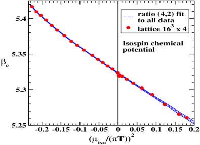
We have tried several kind of interpolations of the pseudocritical couplings at . At first, we have considered interpolations with polynomials up to order (see Table 2, 3rd to 6th rows, for a summary of the resulting fit parameters). We can see that data at are precise enough to be sensitive to terms beyond the order ; indeed, a good /d.o.f. is not achieved before including terms up to the order .
| /d.o.f. | |||||||
|---|---|---|---|---|---|---|---|
| 0.60 | |||||||
| 0.96 | |||||||
| 18.3 | 0 | ||||||
| 0.59 | 0 | ||||||
| 1.85 | 0 | ||||||
| 0.43 | 0 | ||||||
| 0.62 | 0 | ||||||
| 0.49 | 0 |
As in Ref. cea2 , we performed a “constrained” fit: first, the largest interval was identified where data could be interpolated by a first order polynomial in , with a /d.o.f ; it turned out that . Then, all available data were fitted by a 6th-order polynomial, with the constant term and the quadratic coefficient fixed at and , respectively (see Table 2, 7th row).
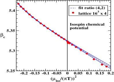
Then, we have considered interpolations with ratios of polynomials of order up to . The interpolation with the least number of parameters for which we got a good fit is the ratio of a 4th- to 2nd-order polynomial, see Table 2, 8th row and Fig. 2(left).
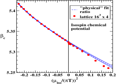
Finally, we have tried here the fit strategy first suggested in Ref. cea2 , consisting in writing the interpolating function in physical units and to deduce from it the functional dependence of on , after establishing a suitable correspondence between physical and lattice units. The natural, dimensionless variables of our theory are , where is the pseudocritical temperature at zero chemical potential, and . The ratio is deduced from the relation , where is the number of lattice sites in the temporal direction and is the lattice spacing at a given . Strictly speaking the lattice spacing depends also on the bare quark mass, however in the following evaluation, which is only based on the perturbative 2-loop expression of for and , we shall neglect such dependence.
We considered the following “physical” fit ratio ():
| (3) |
leading to the following implicit relation between and :
| (4) |
with these resulting parameters
| (5) |
and /d.o.f.=0.53. In Fig. 2(right) we compare the “physical” fit ratio to data for .
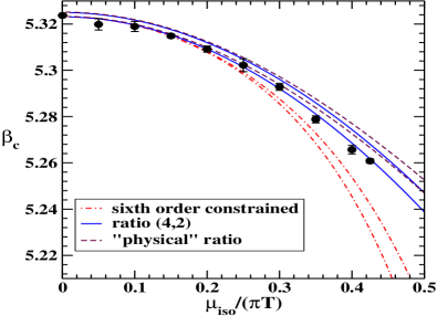
In Fig. 3 we have plotted the extrapolations to the interval of the following fits:
-
•
6th-order constrained polynomial (7th row in Table 2);
-
•
ratio (4,2) of polynomials (last row in Table 2);
- •
The three curves agree as long as , but then the 6th-order constrained polynomial deviates from the other two curves. This means that different interpolations, which all reproduce the trend of data in the fit region and take correctly into account the deviation from the quadratic behavior in that region, lead to distinct extrapolations, as it occurred in SU(3). We can see that ratio of polynomials (Padé approximants) in general tend to be closer to direct determinations of the pseudocritical couplings, which are reported in the same figure for a few values of .
II.2 Nonzero quark chemical potential
| Im | |
|---|---|
In Table 3 we summarize our determinations of the pseudocritical couplings. We have tried several kinds of interpolation of the pseudocritical couplings at . At first, we have considered interpolations with polynomials up to order (see Table 4, 1st to 4th row, for a summary of the resulting fit parameters). We can see that data at are precise enough to be sensitive to terms beyond the order ; indeed, a good /d.o.f. is not achieved before including terms up to the order .
As in the case of isospin chemical potential, we have performed a “constrained” fit. The largest interval for which a linear fit in works well is with ; we notice that such interval was larger () in the case of an isospin chemical potential. Then, all available data were fitted by a 6th-order polynomial, with the constant term and the quadratic coefficient fixed at and , respectively (see Table 4, 5th row).
| /d.o.f. | ||||||
|---|---|---|---|---|---|---|
| 2.87 | ||||||
| 0.63 | ||||||
| 0.85 | ||||||
| 1.41 | ||||||
| 0.65 | ||||||
| 0.60 |
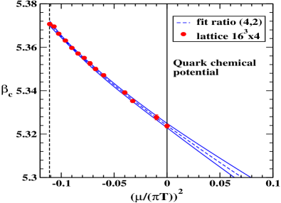
Then, we have considered interpolations with ratios of polynomials: the one with the least number of parameters for which we got a good fit is the ratio of a 4th- to 2nd-order polynomial (see Table 4, 6th row, and Fig. 4(left)).
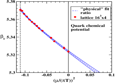
Finally, we have also tried the “physical” fit, as in the previous subsection, obtaining the following results for the “physical” fit ratio, Eq. (3):
| (6) |
with /d.o.f.=0.51, see Fig. 4(right) for a comparison of the fit to data for .
Such interpolation permits, in principle, an extrapolation to real chemical potentials down to ; from the parameters given in (6) one can get the extrapolation at of the pseudocritical quark chemical potential: = 3.284(65) . This result agrees within errors with the analogous one obtained in Ref. NN2011 for SU(3) with Wilson fermions on a smaller lattice and with smaller statistics, which turned out to be 2.73(58) .
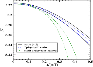
However, a comparison of different extrapolations shows that systematic effects become important well before one approaches the axis. In Fig. 5 we have plotted the extrapolations to the interval of the following fits:
-
•
6th-order constrained polynomial (5th row in Table 4);
-
•
ratio (4,2) of polynomials (last row in Table 4);
- •
The three curves agree as long as , but then the 6th-order constrained polynomial deviates from the other two curves. Therefore results extrapolated to larger values of are not reliable. One could take the analogous results obtained at finite isospin chemical potential as a guiding reference, concluding that Padé like fits are to be preferred; however one cannot exclude that such argument may be wrong because of possible systematic differences between QCD at finite quark and isospin chemical potentials.
III Comparison of the curvatures of the critical lines
In the present Section we will focus on the curvature of the pseudocritical line at , which is the quantity with the least ambiguity related to the procedure of analytic continuation and for which a clear agreement among the determinations obtained by various different methods has been shown in previous literature krato ; fodor . Our purpose is to determine how it changes when switching from a theory at finite quark chemical potential to a theory at finite isospin chemical potential.
In particular we want to determine the dependence of the critical temperature at the quadratic order in and , which is determined by the two curvatures alone. Indeed one can show that, for two degenerate flavors, the theory must be even under reflection of and separately (see Ref. 2im for a discussion on this point), so that the mixed term is absent and
| (7) |
In order to determine the two curvatures and compare them in a consistent way, we have performed a common fit to all the pseudocritical couplings at imaginary potentials reported in Tables 1 and 3 with the following function
| (8) |
including as many data points, both at imaginary and real (when available) chemical potentials, as compatible with a reasonable value of /d.o.f. As a matter of fact the ranges of included chemical potentials coincide with those for which a linear fit works well separately for or (see the second row of Tables 2 and 4), the only difference in this case being that is taken as a common parameter. The results of the fit are
| (9) |
We notice that and are not compatible within errors and deviate from each other by about 4.
A convenient way to report the two curvatures is in term of dimensionless quantities, as follows:
| (10) |
The parameters and can be obtained respectively from and , in particular one has
| (11) | |||||
where is the lattice spacing and is the lattice beta-function. Making use of the perturbative two-loop expression for , we get
| (12) |
It is interesting to compare our results with those of previous studies. In Ref. kogut_curvature the same discretization and bare quark mass have been adopted for QCD at real isospin chemical potential; their result, when reported in the same units as ours, is : the marginal discrepancy can be explained in terms of either the inexact R-algorithm or the smaller spatial volume used in Ref. kogut_curvature . has been obtained in Ref. muim for the same theory with a smaller fermion mass, : this is compatible with our result, showing that has mild dependence on the quark mass. In Ref. NN2011 a value has been reported making use of Wilson fermions: the agreement, even if within quite large errors, is encouraging if we consider the completely different fermion discretization. Instead, as it is well known, the curvature changes significantly if we change the number of flavors; for instance for QCD one obtains immu_dl ; cea3 .
Our determinations of and are clearly affected by the systematic error related to the choice of the two-loop expression for , anyway such error disappears if we consider the ratio
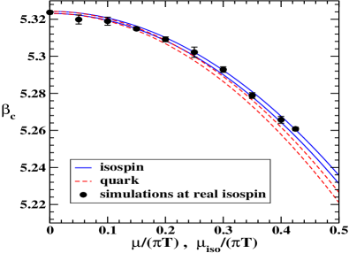
| (13) |
which we consider as our final estimate for the difference in the curvature of the critical line between the theory at finite baryon density and the theory at finite isospin density. In order to appreciate the difference, in Fig. 6 we report the corresponding linear extrapolations to real chemical potentials.
In previous studies the two curvatures revealed to be compatible within errors taylor1 ; kogut_curvature . This is also the expectation in the limit of a large number of colors toublan ; largen1 ; largen2 ; largen3 : indeed the two curvatures are expected to be the same at the leading order toublan (the curvature itself is expected to vanish as ). Therefore, we can consider the deviation that we find as the first evidence for an difference between the two theories at small chemical potentials. , being the ratio of an to an quantity, is expected to be : this is compatible with the fact that it turns out to be of the order of 10%. It would be interesting to explore how results change for different values of .
IV Order of the phase transition
As already stressed in the Introduction, the nature of the pseudocritical line at imaginary , may be strongly influenced by the order of the RW endpoint rwep ; rwep_nf3 ; rwep2 ; rwep3 , i.e. the point at which the RW line taking place in the high- region for Im meets the analytic continuation of the physical pseudocritical line. If the endpoint is first order then it is actually a triple point and at least the part of the pseudocritical line which is closest to the endpoint is expected to be first order.
In the case of , with the same regularization and temporal size () used in the present study, it is known that the RW endpoint is first order, in the low mass region, for with rwep2 . That means that the mass used in the present work, , is close to the tricritical value but slightly on the second order side, so we do not expect the analytic continuation of the pseudocritical line to become first order as we approach the RW endpoint. This is compatible with the fact that we have not observed signals of metastable behavior or double peak distributions along the line; only a strengthening of the transition can be seen as the RW endpoint is approached, as a consequence of the closeness of the tricritical point.
If one conjectures that an imaginary may strengthen the transition in the same way as an imaginary does, then, since the range available for Im is larger than that available for Im, one may expect that a first order transition could be manifest at some stage along the pseudocritical line at imaginary . Such conjecture is well founded, since simulations at real isospin chemical potential have shown that indeed the effect of small positive values of is a weakening of the transition wenger ; kogut_3flv .
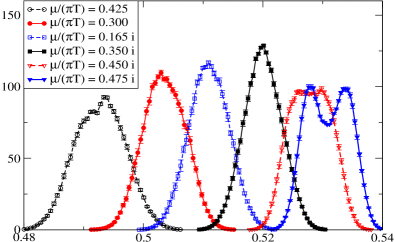
In order to explore this possibility, we have reported in Fig. 7 the plaquette distributions at the pseudocritical coupling for a few different values (both real and imaginary) of . It is evident that for the largest values of a double peak structure develops, hinting at the presence of a first order transition.
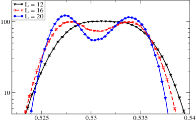
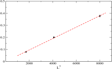
In order to confirm that by a finite size scaling analysis, we have repeated simulations for the largest value of Im, , on two other lattice sizes, and . Both the scaling of distributions and the scaling of susceptibilities confirm the first order nature of the transition for this value of : the well in the double peak distribution of the plaquette deepens as increases as expected (see Fig. 8) and the maxima of the plaquette susceptibility scale linearly with the spatial volume (see Fig. 9).
Therefore we conclude that, for the present discretization and value of the quark mass, the transition is surely first order at and there is possibly a critical point along the line at some smaller value of Im. Such non-trivial behavior resembles what happens for quark chemical potentials rwep ; rwep_nf3 ; rwep2 ; rwep3 and may have consequences on the general structure of the QCD phase diagram which should be further investigated in the future.
V Conclusions
In this paper we have considered QCD with two degenerate flavors of bare mass , corresponding to a pion mass MeV, on a lattice, at nonzero quark or isospin density.
Our investigation developed along three main lines:
-
•
localization of the pseudocritical line in the temperature-chemical potential plane, for the two cases of quark and isospin density;
-
•
comparison of the curvatures of the two critical lines at the point of zero chemical potential;
-
•
study of the order of the phase transition along the two critical lines.
To study the localization of the critical line we adopted the method of analytic continuation. The result we got is similar to what we found in the case of four degenerate flavors and is common to the case of quark and isospin density: deviations from the linear behavior in of the critical lines are clearly seen for and are nicely described by several analytic functions. However, the extrapolations to positive overlap, within errors, only as long as and . The comparison with direct numerical simulations performed at real isospin chemical potentials leads to a preference for extrapolations based on Padé approximants; such suggestion, which is agreement with our previous studies, could be taken as a guiding principle also in the case of nonzero quark density.
We have performed a careful determination of the curvatures of the two critical lines at zero chemical potential. In order to compare them in a consistent way, we have performed a common fit of the pseudocritical couplings, taking the critical at zero chemical potential as a common parameter. We have found that the curvature of the isospin critical line is larger than that of the quark critical line by about 4, the relative difference being about 10%. The outcome of previous studies taylor1 ; kogut_curvature was in favour of a substantial agreement between the two curvatures, as expected in the limit of a large number of colors toublan ; largen1 ; largen2 ; largen3 and in particular at the leading order toublan . The deviation that we find is therefore a first evidence for an difference between the two theories at small chemical potentials. The order of magnitude of the relative deviation , which is the ratio of an to an quantity (the curvature itself) is compatible with it being an quantity. It would be interesting to explore how results change for different values of .
Finally, we have studied the order of the transitions along the critical lines. For the case of nonzero quark density, we have found no clear signatures of a first order transition, in agreement with the expectations after recent findings in the literature and in consideration of the quark mass adopted in this work, which is larger than the tricritical mass found in Ref. rwep2 . The only effect we could see was a strengthening of the transition when the RW point is approached at imaginary quark chemical potential.
A phenomenon emerged from our investigation is instead that an imaginary isospin chemical potential can strengthen the transition, similarly to what happens for a quark chemical potential and in agreement with the fact that simulations at real isospin chemical isospin have shown that small positive values of weaken the transition wenger ; kogut_3flv . Moreover we have found clear evidence that, in this case, the transition becomes first order for large enough imaginary chemical potentials, but before one reaches the RW-like transition which is found, in the high- region, for cea2 , implying a possible second order critical point along the line. Such behavior is very similar to what found for a quark chemical potential, hinting at a common underlying physical mechanism, and could have various non-trivial consequences, on the shape of the critical line and on the general structure of the QCD phase diagram, that should be further investigated in future studies.
VI Acknowledgments
We are grateful to Claudio Bonati, Philippe de Forcrand and Owe Philipsen for useful discussions. We acknowledge the use of the PC clusters of the INFN Bari Computer Center for Science and of the INFN-Genova Section.
References
- (1) D.T. Son and M.A. Stephanov, Phys. Rev. Lett. 86, 592 (2001).
- (2) J.B. Kogut and D.K. Sinclair, Phys. Rev. D 66, 034505 (2002).
- (3) M.G. Alford, A. Kapustin, and F. Wilczek, Phys. Rev. D 59, 054502 (1999).
- (4) M.-P. Lombardo, Nucl. Phys. Proc. Suppl. 83, 375 (2000).
- (5) Ph. de Forcrand and O. Philipsen, Nucl. Phys. B 642, 290 (2002); Nucl. Phys. B 673, 170 (2003).
- (6) M. D’Elia and M.P. Lombardo, Phys. Rev. D 67, 014505 (2003); Phys. Rev. D 70, 074509 (2004).
- (7) V. Azcoiti, G. Di Carlo, A. Galante and V. Laliena, Nucl. Phys. B 723, 77 (2005).
- (8) H.S. Chen, X.Q. Luo, Phys. Rev. D 72, 034504 (2005).
- (9) Ph. de Forcrand and O. Philipsen, JHEP 0701, 077 (2007); JHEP 0811, 012 (2008); PoS LAT 2007, 178 (2007).
- (10) M. D’Elia, F. Di Renzo, M.P. Lombardo, Phys. Rev. D 76, 114509 (2007).
- (11) M. D’Elia and F. Sanfilippo, Phys. Rev. D 80, 014502 (2009).
- (12) P. Cea, L. Cosmai, M. D’Elia and A. Papa, Phys. Rev. D 81, 094502 (2010); PoS LATTICE 2010, 173 (2010).
- (13) L.K. Wu, X.Q. Luo and H.S. Chen, Phys. Rev. D 76, 034505 (2007).
- (14) K. Nagata and A. Nakamura, Phys. Rev D 83, 114507 (2011).
- (15) A. Hart, M. Laine, and O. Philipsen, Phys. Lett. B 505, 141 (2001).
- (16) P. Giudice and A. Papa, Phys. Rev. D 69, 094509 (2004); Nucl. Phys. Proc. Suppl. 140, 529 (2005).
- (17) P. Cea, L. Cosmai, M. D’Elia and A. Papa, JHEP 0702, 066 (2007); PoS LAT 2006, 143 (2006).
- (18) P. Cea, L. Cosmai, M. D’Elia and A. Papa, Phys. Rev. D 77, 051501 (2008); PoS LAT 2007, 214 (2007); PoS LAT 2009, 192 (2009).
- (19) S. Conradi, M. D’Elia, Phys. Rev. D 76, 074501 (2007).
- (20) Y. Shinno and H. Yoneyama, arXiv:0903.0922 [hep-lat].
- (21) P. Cea, L. Cosmai, M. D’Elia, C. Manneschi and A. Papa, Phys. Rev. D 80, 034501 (2009); PoS LAT 2009, 161 (2009).
- (22) S. Kim, P. de Forcrand, S. Kratochvila, and T. Takaishi, PoS LAT 2005, 166 (2006).
- (23) F. Karbstein, M. Thies, Phys. Rev. D 75, 025003 (2007).
- (24) A. Roberge, N. Weiss, Nucl. Phys. B 275, 734 (1986).
- (25) P. de Forcrand and O. Philipsen, JHEP 0811, 012 (2008).
- (26) M. D’Elia and F. Sanfilippo, Phys. Rev. D 80, 111501 (2009).
- (27) P. de Forcrand and O. Philipsen, Phys. Rev. Lett. 105, 152001 (2010).
- (28) C. Bonati, G. Cossu, M. D’Elia and F. Sanfilippo, Phys. Rev. D 83, 054505 (2011).
- (29) C. Bonati, P. de Forcrand, M. D’Elia, O. Philipsen and F. Sanfilippo, arXiv:1201.2769 [hep-lat].
- (30) H. Kouno, Y. Sakai, K. Kashiwa and M. Yahiro, J. Phys. G 36, 115010 (2009).
- (31) J. Braun, L. M. Haas, F. Marhauser and J. M. Pawlowski, Phys. Rev. Lett. 106, 022002 (2011).
- (32) Y. Sakai, H. Kouno, M. Yahiro, J. Phys. G 37, 105007 (2010).
- (33) G. Aarts, S. P. Kumar and J. Rafferty, JHEP 1007, 056 (2010).
- (34) J. M. Pawlowski, AIP Conf. Proc. 1343, 75 (2011).
- (35) H. Kouno, Y. Sakai, T. Sasaki, K. Kashiwa and M. Yahiro, Phys. Rev. D 83, 076009 (2011).
- (36) J. Rafferty, JHEP 1109, 087 (2011).
- (37) V. Pagura, D. G. Dumm and N. N. Scoccola, Phys. Lett. B 707, 76 (2012).
- (38) K. Kashiwa, T. Hell and W. Weise, Phys. Rev. D 84, 056010 (2011).
- (39) K. Morita, V. Skokov, B. Friman and K. Redlich, Phys. Rev. D 84, 076009 (2011).
- (40) P. Cea, L. Cosmai, M. D’Elia, A. Papa and F. Sanfilippo, PoS LATTICE 2011, 187 (2011).
- (41) M.-P. Lombardo, PoS LAT 2005, 168 (2006).
- (42) S. Kratochvila and P. de Forcrand, PoS LAT 2005, 167 (2006).
- (43) Z. Fodor and S. D. Katz, arXiv:0908.3341 [hep-ph].
- (44) J.B. Kogut and D.K. Sinclair, Phys. Rev. D 70, 094501 (2004).
- (45) C.R. Allton et al., Phys. Rev. D 66, 074507 (2002).
- (46) D. Toublan, Phys. Lett. B 621, 145 (2005).
- (47) M. Hanada and N. Yamamoto, arXiv:1103.5480 [hep-ph].
- (48) M. Hanada, arXiv:1109.6372 [hep-lat].
- (49) M. Hanada, C. Hoyos, A. Karch and L. G. Yaffe, arXiv:1201.3718 [hep-th].
- (50) J.B. Kogut and D.K. Sinclair, Phys. Rev. D 77 114503 (2008).
- (51) P. de Forcrand, M. A. Stephanov and U. Wenger, PoS LAT 2007, 237 (2007) [arXiv:0711.0023 [hep-lat]].