Training Restricted Boltzmann Machines on Word Observations

Abstract

The restricted Boltzmann machine (RBM) is a flexible model for complex data. However, using RBMs for high-dimensional multinomial observations poses significant computational difficulties. In natural language processing applications, words are naturally modeled by $K$-ary discrete distributions, where $K$ is determined by the vocabulary size and can easily be in the hundred thousands. The conventional approach to training RBMs on word observations is limited because it requires sampling the states of $K$-way softmax visible units during block Gibbs updates, an operation that takes time linear in $K$. In this work, we address this issue with a more general class of Markov chain Monte Carlo operators on the visible units, yielding updates with computational complexity independent of $K$. We demonstrate the success of our approach by training RBMs on hundreds of millions of word $n$-grams using larger vocabularies than previously feasible with RBMs and by using the learned features to improve performance on chunking and sentiment classification tasks, achieving state-of-the-art results on the latter.

1 Introduction

The breadth of applications for the restricted Boltzmann machine (RBM) (Smolensky, 1986; Freund and Haussler, 1991) has expanded rapidly in recent years. For example, RBMs have been used to model image patches (Ranzato et al., 2010), text documents as bags of words (Salakhutdinov and Hinton, 2009), and movie ratings (Salakhutdinov et al., 2007), among other data. Although RBMs were originally developed for binary observations, they have been generalized to several other types of data, including integer- and real-valued observations (Welling et al., 2005).

However, one type of data that is not well supported by the RBM is word observations from a large vocabulary (e.g., 100,000 words). The issue is not one of representing such observations in the RBM framework: so-called softmax units (Salakhutdinov and Hinton, 2009) are the natural choice for modeling words. The issue is that manipulating distributions over the states of such units is expensive even for intermediate vocabulary sizes and becomes impractical for vocabulary sizes in the hundred thousands — a typical situation for NLP problems. For example, with a vocabulary of 100,000 words, modeling $n$-gram windows of size ${n=5}$ is comparable in scale to training an RBM on binary vector observations of dimension 500,000 (i.e., more dimensions than a ${700\times 700}$ pixel image). This scalability issue has been a primary obstacle to using the RBM for natural language processing.

In this work, we directly address the scalability issues associated with large softmax visible units in RBMs. We describe a learning rule with a computational complexity independent of the number of visible units. We obtain this rule by replacing the Gibbs sampling transition kernel over the visible units with carefully implemented Metropolis–Hastings transitions. By training RBMs in this way on hundreds of millions of word windows, they learn representations capturing meaningful syntactic and semantic properties of words. Our learned word representations provide benefits on a chunking task competitive with other methods of inducing word representations and our learned $n$-gram features yield even larger performance gains. Finally, we also show how similarly extracted $n$-gram representations can be used to obtain state-of-the-art performance on a sentiment classification benchmark.

2 Restricted Boltzmann Machines

We first describe the restricted Boltzmann machine for binary observations, which provides the basis for other data types. An RBM defines a distribution over a binary visible vector ${\mathbf{v}}$ of dimensionality $V$ and a layer ${\mathbf{h}}$ of $H$ binary hidden units through an energy

$$E({\mathbf{v}},{\mathbf{h}})=-{\mathbf{b}}^{\top}{\mathbf{v}}-{\mathbf{c}}^{\top}{\mathbf{h}}-{\mathbf{h}}^{\top}{\mathbf{W}}{\mathbf{v}}.$$ (1)

This energy is parameterized by bias vectors ${{\mathbf{b}}\in{\mathbb{R}}^{V}}$ and ${{\mathbf{c}}\in{\mathbb{R}}^{H}}$ and weight matrix ${{\mathbf{W}}\in{\mathbb{R}}^{H\times V}}$, and is converted into a probability distribution via

$$p({\mathbf{v}},{\mathbf{h}}) =\exp\left(-E({\mathbf{v}},{\mathbf{h}})\right)\,/\,Z$$ (2)

$$Z =\sum_{{\mathbf{v}}^{\prime},{\mathbf{h}}^{\prime}}\exp(-E({\mathbf{v}}^{\prime},{\mathbf{h}}^{\prime}))~{}.$$ (3)

This yields simple conditional distributions:

$$p({\mathbf{h}}|{\mathbf{v}}) =\prod_{j}p(h_{j}|{\mathbf{v}}) p({\mathbf{v}}|{\mathbf{h}}) =\prod_{i}p(v_{i}|{\mathbf{h}})$$ (4)

$$p(h_{j}=1|{\mathbf{v}}) ={\rm sigm}(c_{j}+\sum_{i}W_{ji}v_{i})$$ (5)

$$p(v_{i}=1|{\mathbf{h}}) ={\rm sigm}(b_{i}+\sum_{j}W_{ji}h_{j}),$$ (6)

where ${\rm sigm}(z)=1/(1+e^{-z})$, which allow for efficient Gibbs sampling of each layer given the other layer.

We train an RBM from $T$ visible data vectors $\{{\mathbf{v}}_{t}\}^{T}_{t=1}$ by minimizing the scaled negative (in practice, penalized) log likelihood of the parameters ${\theta=({\mathbf{b}},{\mathbf{c}},{\mathbf{W}})}$:

$$\theta_{\sf{MLE}} =\underset{\theta}{\operatorname{argmin}}\;{\cal L(\theta)} {\cal L(\theta)} =\frac{1}{T}\sum_{t}\ell({\mathbf{v}}_{t};\theta)$$ (7)

$$\ell({\mathbf{v}}_{t};\theta) =-\log p({\mathbf{v}}_{t})=-\log\sum_{{\mathbf{h}}}p({\mathbf{v}}_{t},{\mathbf{h}}).$$ (8)

The gradient of the objective with respect to $\theta$

$$\frac{\partial{\cal L}(\theta)}{\partial\theta} =\frac{1}{T}\sum_{t}\mathbb{E}_{{\mathbf{h}}|{\mathbf{v}}_{t}}\left[\frac{\partial E({\mathbf{v}}_{t},{\mathbf{h}})}{\partial\theta}\right]-\mathbb{E}_{{\mathbf{v}},{\mathbf{h}}}\left[\frac{\partial E({\mathbf{v}},{\mathbf{h}})}{\partial\theta}\right]$$

is intractable to compute because of the exponentially many terms in the sum over joint configurations of the visible and hidden units in the second expectation.

Fortunately, for a given $\theta$, we can approximate this gradient by replacing the second expectation with a Monte Carlo estimate based on a set of $M$ samples ${{\cal N}=\{\tilde{{\mathbf{v}}}_{m}\}}$ from the RBM’s distribution:

$$\mathbb{E}_{{\mathbf{v}},{\mathbf{h}}}\left[\frac{\partial E({\mathbf{v}},{\mathbf{h}})}{\partial\theta}\right] \approx\frac{1}{M}\!\!\sum_{\tilde{{\mathbf{v}}}_{m}\in{\cal N}}\!\!\mathbb{E}_{{\mathbf{h}}|\tilde{{\mathbf{v}}}_{m}}\!\!\left[\frac{\partial E(\tilde{{\mathbf{v}}}_{m},{\mathbf{h}})}{\partial\theta}\right]~{}.$$ (9)

The samples $\{\tilde{{\mathbf{v}}}_{m}\}$ are often referred to as “negative samples” as they counterbalance the gradient due to the observed, or “positive” data. To obtain these samples, we maintain $M$ parallel Markov chains throughout learning and update them using Gibbs sampling between parameter updates.

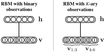
Figure 1: Illustration of an RBM with binary observations (left) and $K$-ary observations, for $n=2$ and $K=3$, i.e. a pair of $3$-ary observations (right).

Learning with the Monte Carlo estimator alternates between two steps: 1) Using the current parameters $\theta$, simulate a fews steps of the Markov chain on the $M$ negative samples using Eqs. (4)-(6); and 2) Using the negative samples, along with a mini-batch (subset) of the positive data, compute the gradient in Eq. (9) and update the parameters. This procedure belongs to the general class of Robbins-Monro stochastic approximation algorithms (Younes, 1989). Under mild conditions, which include the requirement that the Markov chain operators leave $p({\mathbf{v}},{\mathbf{h}}\,|\,\theta)$ invariant, this procedure will converge to a stable point of ${\cal L}(\theta)$.

For $K$-ary observations — observations belonging to a finite set of $K$ discrete outcomes — we can use the same energy function as in Eq. (1) for the binary RBM by encoding each observation in a “one-hot” representation and concatenating the representations of all observations to construct ${\mathbf{v}}$. In other words, for $n$ separate $K$-ary observations, the visible units ${\mathbf{v}}$ will be partitioned into $n$ groups of $K$ binary units, with the constraint that each partition can only contain a single non-zero entry. Using the notation ${\mathbf{v}}_{a:b}$ to refer to the subvector of elements from index $a$ to index $b$, the $i^{\rm th}$ observation will then be encoded by the group of visible units ${\mathbf{v}}_{(i-1)K+1:iK}$. The one-hot encoding is enforced by constraining each group of units to contain only a single 1-valued unit, the others being set to 0. The difference between RBMs with binary and $K$-ary observations is illustrated in Figure 1.

To simplify notation, we refer to the $i^{\rm th}$ group of visible units as ${{\mathbf{v}}^{(i)}\!=\!{\mathbf{v}}_{(i-1)K+1:iK}}$. Similarly, we will refer to the biases and weights associated with those units as ${{\mathbf{b}}^{(i)}={\mathbf{b}}_{(i-1)K+1:iK}}$ and ${{\mathbf{W}}^{(i)}={\mathbf{W}}_{\cdot,(i-1)K+1:iK}}$. We will also denote with ${\mathbf{e}}_{k}$ the one-hot vector with its $k^{\rm th}$ component set to 1.

The conditional distribution over the visible layer is

$$p({\mathbf{v}}|{\mathbf{h}}) =\prod_{i=1}^{n}p({\mathbf{v}}^{(i)}|{\mathbf{h}})$$ (10)

$$p({\mathbf{v}}^{(i)}\!=\!{\mathbf{e}}_{k}|{\mathbf{h}}) =\frac{\exp({\mathbf{b}}^{(i)^{\top}}{\mathbf{e}}_{k}+{\mathbf{h}}^{\top}{\mathbf{W}}^{(i)}{\mathbf{e}}_{k})}{\sum_{k^{\prime}}\exp({\mathbf{b}}^{(i)i^{\top}}{\mathbf{e}}_{k^{\prime}}\!+\!{\mathbf{h}}^{\top}{\mathbf{W}}^{(i)}{\mathbf{e}}_{k^{\prime}})}.$$

Each group ${\mathbf{v}}^{(i)}$ has a multinomial distribution given the hidden layer. Because the multinomial probabilities are given by a softmax nonlinearity, the group of units ${\mathbf{v}}^{(i)}$ are referred to as softmax units (Salakhutdinov and Hinton, 2009).

3 Difficulties with Word Observations

While in the binary case the size of the visible layer is equal to data dimenionality, in the $K$-ary case the size of the visible layer is $K$ times the dimensionality. For language processing applications, where $K$ is the vocabulary size and can run into the hundred thousands, the visible layer can become unmanageably large.

The difficulty with large $K$ is that the Gibbs operator on the visible units becomes expensive to simulate, making it difficult to perform updates of the negative samples. That is, generating a sample from the conditional distribution in Eq. (10) dominates the stochastic learning procedure as $K$ increases. The reason for this expense is that it is necessary to compute the activity associated with each of the $K$ possible outcomes, even though only a single one will actually be selected.

On the other hand, given a mini-batch $\{{\mathbf{v}}_{t}\}$ and negative samples $\{\tilde{{\mathbf{v}}}_{m}\}$, the gradient computations in Eq. (9) are able to take advantage of the sparsity of the visible activity. Since each ${\mathbf{v}}_{t}$ and $\tilde{{\mathbf{v}}}_{m}$ only contain $n$ non-zero entries, the cost of the gradient estimator has no dependence on $K$ and can be rapidly computed. Thus the only barrier to efficient learning of high-dimensional multinomial RBMs is the complexity of the Gibbs update for the visible units.

Dealing with large multinomial distributions is an issue that has come up previously in work on neural network language models (Bengio et al., 2001). For example, Morin and Bengio (2005) addressed this problem by introducing a fixed factorization of the (conditional) multinomial using a binary tree in which each leaf is associated with a single word. The tree was determined using an external knowledge base, although Mnih and Hinton (2009) investigated ways of extending this approach by learning the word tree from data.

Unfortunately, tree-structured solutions are not applicable to the problem of modeling the joint distribution of $n$ consecutive words, as we wish to do here. Introducing a directed tree breaks the undirected, symmetric nature of the interaction between the visible and hidden units of the RBM. While one strategy might be to use a conditional RBM to model the tree-based factorizations, similar to Mnih and Hinton (2009), the end result would not be an RBM model of $n$-gram word windows, nor would it even be a conditional RBM over the next word given the $n-1$ previous ones.

In summary, dealing with $K$-ary observations in the Boltzmann machine framework for large $K$ is a crucial open problem that has inhibited the development of deep learning solutions NLP problems.

4 Metropolis–Hastings for Softmax Units

Having identified the Gibbs update of the visible units as the limiting factor in efficient learning of large-$K$ multinomial observations, it is natural to examine whether other operators might be used for the Monte Carlo estimate in Eq. (9). In particular, we desire a transition operator that can take advantage of the same sparse operations that enable the gradient to be efficiently computed from the positive and negative samples, while still leaving $p({\mathbf{v}},{\mathbf{h}})$ invariant and thus still satisfying the convergence conditions of the stochastic approximation learning procedure.

To achieve this, instead of sampling exactly from the conditionals $p({\mathbf{v}}^{(i)}|{\mathbf{h}})$ within the Markov chain, we use a small number of iterations of Metropolis–Hastings (M–H) sampling. Let $q(\hat{{\mathbf{v}}}^{(i)}\leftarrow{\mathbf{v}}^{(i)})$ be a proposal distribution for group $i$. The following stochastic operator leaves $p({\mathbf{v}},{\mathbf{h}})$ invariant:

1. Given the current visible state ${\mathbf{v}}$, sample a proposal $\hat{{\mathbf{v}}}$ for group $i$, such that ${\hat{{\mathbf{v}}}^{(i)}\sim q(\hat{{\mathbf{v}}}^{(i)}\leftarrow{\mathbf{v}}^{(i)})}$ and ${\hat{{\mathbf{v}}}^{(j)}={\mathbf{v}}^{(j)}}$ for ${i\neq j}$ (i.e. sample a proposed new word for position $i$).

2. Replace the $i$th part of the current state ${\mathbf{v}}^{(i)}$ with $\hat{{\mathbf{v}}}^{(i)}$ with probability:

$$\min\left\{1,\frac{q({\mathbf{v}}^{(i)}\leftarrow\hat{{\mathbf{v}}}^{(i)})\exp({\mathbf{b}}^{(i)^{\top}}\hat{{\mathbf{v}}}^{(i)}+{\mathbf{h}}^{\top}{\mathbf{W}}^{(i)}\hat{{\mathbf{v}}}^{(i)})}{q(\hat{{\mathbf{v}}}^{(i)}\leftarrow{\mathbf{v}}^{(i)})\exp({\mathbf{b}}^{(i)^{\top}}{\mathbf{v}}^{(i)}+{\mathbf{h}}^{\top}{\mathbf{W}}^{(i)}{\mathbf{v}}^{(i)})}\right\}.$$

Assuming it is possible to efficiently sample from the proposal distribution  ${q(\hat{{\mathbf{v}}}^{(i)}\leftarrow{\mathbf{v}}^{(i)})}$, this M–H operator is fast to compute as it does not require normalizing over all possible values of the visible units in group $i$ and, in fact, only requires the unnormalized probability of one of them. Moreover, as the $n$ visible groups are conditionally independent given the hiddens, each group can be simulated in parallel (i.e., words are sampled at every position separately). The efficiency of these operations make it possible to apply this transition operator many times before moving on to other parts of the learning and still obtain a large speedup over exact sampling from the conditional.

4.1 Efficient Sampling of Proposed Words

The utility of M–H sampling for an RBM with word observations relies on the fact that sampling from the proposal $q(\hat{{\mathbf{v}}}^{(i)}\!\leftarrow\!{\mathbf{v}}^{(i)})$ is much more efficient than sampling from the correct softmax multinomial. Although there are many possibilities for designing such proposals, here we will explore the most basic variant: independence chain Metropolis–Hastings in which the proposal distribution is fixed to be the marginal distribution over words in the corpus.

Naïve procedures for sampling from discrete distributions typically have linear time complexity in the number of outcomes. However, the alias method (pseudocode at www.cs.toronto.edu/~gdahl) of Kronmal and Perterson (1979) can be used to generate samples in constant time with linear setup time. While the alias method would not help us construct a Gibbs sampler for the visibles, it does make it possible to generate proposals extremely efficiently, which we can then use to simulate the Metropolis–Hastings operator, regardless of the current target distribution.

The alias method leverages the fact that any $K$-valued discrete distribution can be written as a uniform mixture of $K$ Bernoulli distributions. Having constructed this mixture distribution at setup time (with linear time and space cost), new samples can be generated in constant time by sampling uniformly from the $K$ mixture components, followed by sampling from that component’s Bernoulli distribution.

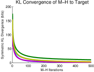
(a) Example KL Convergence

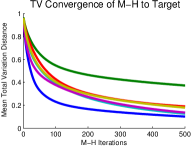
(b) Example TV Convergence

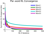
(c) Example Per-Word KL

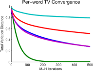
(d) Example Per-Word TV

Figure 2: Convergence of the Metropolis–Hastings operator to the true conditional distribution over the visibles for a trained 5-gram RBM with a vocabulary of 100K words. (a) KL divergence for six randomly-chosen data cases. (b) Average total variation distance for the same six cases. (c,d) For the slowest-converging of the six top curves (dark green), these are broken down for each of the five multinomials in KL and total variation, respectively.

4.2 Mixing of Metropolis–Hastings

Although this procedure eliminates dependence of the learning algorithm on $K$, it is important to examine the mixing of Metropolis–Hastings and how sensitive it is to $K$ in practice. Although there is evidence (Hinton, 2002) that poorly-mixing Markov chains can yield good learning signals, when this will occur is not as well understood. We examined the mixing issue using the model described in Section 6.1 with the parameters learned from the Gigaword corpus with a 100,000-word vocabulary as described in Section 6.2.

We analytically computed the distributions implied by iterations of the M–H operator, assuming the initial state was drawn according to $\prod_{i}q({\mathbf{v}}^{(i)})$. As this computation requires the instantiation of $n$ ${100\sf{k}\times 100\sf{k}}$ matrices, it cannot be done at training time, but was done offline for analysis purposes. Each application of Metropolis–Hastings results in a new distribution converging to the target (true) conditional.

Figures 2(a) and 2(b) show this convergence for the “reconstruction” distributions of six randomly-chosen 5-grams from the corpus, using two metrics: symmetric Kullback–Leibler (KL) divergence and total variation (TV) distance, which is the standard measure for analysis of MCMC mixing. The TV distance shown is the mean across the five group distributions. Figures 2(c) and 2(d) show these metrics broken down by grouping, for the slowest curves (dark green) of the top two figures. These curves highlight that the state of the hidden units has a strong impact on the mixing and that most groups mix very quickly while a few converge slowly. We feel that these curves, along with the results of Section 6, indicate that the mixing is effective, but could benefit from further study.

5 Related Work

Using M–H sampling for a multinomial distribution with softmax probabilities has been explored in the context of a neural network language model by Bengio and Sénécal (2003). They used M–H to estimate the training gradient at the output of the neural network. However, their work did not address or investigate its use in the context of Boltzmann machines in general.

Salakhutdinov and Hinton (2009) describe an alternative to directed topic models called the replicated softmax RBM that uses softmax units over the entire vocabulary with tied weights to model an unordered collection of words (a.k.a. bag of words). Since their RBM ties the weights to all the words in a single document, there is only one vocabulary-sized multinomial distribution to compute per document, instead of the $n$ required when modeling a window of consecutive words. Therefore sampling a document conditioned on the hidden variables of the replicated softmax still incurs a computational cost linear in $K$, although the problem is not amplified by a factor of $n$ as it is here. Notably, Salakhutdinov and Hinton (2009) limited their vocabulary to ${K<14,000}$.

No known previous work has attempted to address the computational burden associated with $K$-ary observations with large $K$ in RBMs. The M–H-based approach used here is not specific to a particular Boltzmann machine and could be used for any model with large softmax units, although the applications that motivate us come from NLP. Dealing with the large softmax problem is essential if Boltzmann machines are to be practical for natural language data.

In Section 6, we present results on the task of learning word representations. This task has been investigated previously by others. Turian et al. (2010) provide an overview and evaluation of these different methods, including those of Mnih and Hinton (2009) and of Collobert and Weston (2008). We have already mentioned the work of Mnih and Hinton (2009), who model the conditional distribution of the last word in $n$-gram windows. Collobert and Weston (2008) follows a similar approach, by training a neural network to fill-in the middle word of an $n$-gram window, using a margin-based learning objective. In contrast, we model the joint distribution of the whole $n$-gram window, which implies that the RBM could be used to fill-in any word within a window. Moreover, inference with an RBM yields a hidden representation of the whole window and not simply of a single word.

6 Experiments

We evaluated our M–H approach to training RBMs on two NLP tasks: chunking and sentiment classification. Both applications will be based on the same RBM model over $n$-gram windows of words, hence we first describe the parameterization of this RBM and later present how it was used for chunking and sentiment classification. Both applications also take advantage of the model’s ability to learn useful feature vectors for entire $n$-grams, not just individual words.

6.1 RBM Model of $n$-gram Windows

In the standard parameterization presented in Section 2, the RBM uses separate weights (i.e., different columns of ${\mathbf{W}}$) to model observations at different positions. When training an RBM on word $n$-gram windows, we would prefer to share parameters across identical words in different positions in the window and factor the weights into position-dependent weights and position-independent weights (word representations).

Therefore, we use an RBM parameterization very similar to that of Mnih and Hinton (2007), which itself is inspired by previous work on neural language models (Bengio et al., 2001). The idea is to learn, for each possible word $w$, a lower-dimensional linear projection of its one-hot encoding by incorporating the projection directly in the energy function of the RBM. Moreover, we share this projection across positions within the $n$-gram window. Let ${\mathbf{D}}$ be the matrix of this linear projection and let ${\mathbf{e}}_{w}$ be the one-hot representation of $w$ (where we treat $w$ as an integer index in the vocabulary), performing this projection ${\mathbf{D}}{\mathbf{e}}_{w}$ is equivalent to selecting the appropriate column ${\mathbf{D}}_{\cdot,w}$ of this matrix. This column vector can then be seen as a real-valued vector representation of that word. The real-valued vector representations of all words within the $n$-gram are then concatenated and connected to the hidden layer with a single weight matrix.

More specifically, let ${\mathbf{D}}$ be the ${D\times K}$ matrix of word representations. These word representations are introduced by reparameterizing ${{\mathbf{W}}^{(i)}={\mathbf{U}}^{(i)}{\mathbf{D}}}$, where ${\mathbf{U}}^{(i)}$ is a position-dependent ${H\times D}$ matrix. The biases across positions are also shared, i.e., we learn a single bias vector ${\mathbf{b}}^{*}$ that is used at all positions (${\mathbf{b}}^{(i)}={\mathbf{b}}^{*}~{}\forall i$). The energy function becomes

$$E({\mathbf{v}},{\mathbf{h}})=-{\mathbf{c}}^{\top}{\mathbf{h}}+\sum_{i=1}^{n}-{\mathbf{b}}^{*^{\top}}{\mathbf{v}}^{(i)}-{\mathbf{h}}^{\top}~{}{\mathbf{U}}^{(i)}~{}{\mathbf{D}}{\mathbf{v}}^{(i)}$$

with conditional distributions

$$p({\mathbf{h}}|{\mathbf{v}}) =\prod_{j}p(h_{j}|{\mathbf{v}}) p({\mathbf{v}}|{\mathbf{h}}) =\prod_{i=1}^{n}p({\mathbf{v}}^{(i)}|{\mathbf{h}})$$

$$p(h_{j}=1|{\mathbf{v}}) ={\rm sigm}\left(c_{j}+\sum_{i=1}^{n}{\mathbf{U}}_{j\cdot}^{(i)}~{}{\mathbf{D}}{\mathbf{v}}^{(i)}\right)$$

$$p({\mathbf{v}}^{(i)}={\mathbf{e}}_{k}|{\mathbf{h}}) =\frac{\exp({\mathbf{b}}^{*^{\top}}{\mathbf{e}}_{k}+{\mathbf{h}}^{\top}{\mathbf{U}}^{(i)}~{}{\mathbf{D}}{\mathbf{e}}_{k})}{\sum_{k^{\prime}=1}^{K}\exp({\mathbf{b}}^{*^{\top}}{\mathbf{e}}_{k^{\prime}}+{\mathbf{h}}^{\top}{\mathbf{U}}^{(i)}~{}{\mathbf{D}}{\mathbf{e}}_{k^{\prime}})}$$

where ${\mathbf{U}}_{j\cdot}^{(i)}$ refers to the $j^{\rm th}$ row vector of ${\mathbf{U}}^{(i)}$. The gradients with respect to this parameterization are easily derived from Eq. (9). We refer to this construction as a word representation RBM (WRRBM).

In contrast to Mnih and Hinton (2007), rather than training the WRRBM conditionally to model $p(w_{n+t-1}|w_{t},\dots,w_{n+t-2})$, we train it using Metropolis–Hastings to model the full joint distribution $p(w_{t},\dots,w_{n+t-1})$. That is, we train the WRRBM based on the objective

$${\cal L(\theta)}=\!-\!\sum_{t}\!\log p({\mathbf{v}}^{(1)}\!=\!{\mathbf{e}}_{w_{t}},{\mathbf{v}}^{(2)}\!=\!{\mathbf{e}}_{w_{t+1}},\dots,{\mathbf{v}}^{(n)}_{w_{n+t-1}})$$

using stochastic approximation from M–H sampling of the word observations. For models with ${n>2}$, we also found it helpful to incorporate $\ell_{2}$ regularization of the weights, and to use momentum when updating ${\mathbf{U}}^{(i)}$.

6.2 Chunking Task

As described by Turian et al. (2010), learning real-valued word representations can be used as a simple way of performing semi-supervised learning for a given method, by first learning word representations on unlabeled text and then feeding these representations as additional features to a supervised learning model.

We trained the WRRBM on windows of text derived from the English Gigaword corpus. The dataset is a corpus of newswire text from a variety of sources. We extracted each news story and trained only on windows of $n$ words that did not cross the boundary between two different stories. We used NLTK (Bird et al., 2009) to tokenize the words and sentences, and also corrected a few common punctuation-related tokenization errors. As in Collobert et al. (2011), we lowercased all words and delexicalized numbers (replacing consecutive occurrences of one or more digits inside a word with just a single # character). Unlike Collobert et al. (2011), we did not include additional capitalization features, but discarded all capitalization information. We used a vocabulary consisting of the 100,000 most frequent words plus a special “unknown word” token to which all remaining words were mapped.

We evaluated the learned WRRBM word representations on a chunking task, following the setup described in Turian et al. (2010) and using the associated publicly-available code, as well as CRFSuite. As in Turian et al. (2010), we used data from the CoNLL-2000 shared task. We used a scale of $0.1$ for the word representation features (as Turian et al. (2010) recommend) and for each WRRBM model, tried $\ell_{2}$ penalties ${\lambda\in\{0.0001,1.2,2.4,3.2\}}$ for CRF training. We selected the single model with the best validation F1 score over all runs and evaluated it on the test set. The model with the best validation F1 score used $3$-gram word windows, ${\lambda=1.2}$, 250 hidden units, a learning rate of 0.01, and used 100 steps of M–H sampling to update each word observation in the negative data.

The results are reported in Table 1, where we observe that word representations learned by our model achieved higher validation and test scores than the baseline of not using word representation features, and are comparable to the best of the three word representations tried in Turian et al. (2010).

Although the word representations learned by our model are highly effective features for chunking, an important advantage of our model over many other ways of inducing word representations is that it also naturally produces a feature vector for the entire $n$-gram. For the trigram model mentioned above, we also tried adding the hidden unit activation probability vector as a feature for chunking. For each word $w_{i}$ in the input sentence, we generated features using the hidden unit activation probabilities for the trigram $w_{i-1}w_{i}w_{i+1}$. No features were generated for the first and last word of the sentence. The hidden unit activation probability features improved validation set F1 to 95.01 and test set F1 to 94.44, a test set result superior to all word embedding results on chunking reported in Turian et al. (2010).

Table 1: Comparison of experimental results on the chunking task. The baseline results were taken from Turian et al. (2010). The performance measure is F1.

Model	Valid	Test
CRF w/o word representations	94.16	93.79
HLBL (Mnih and Hinton, 2009)	94.63	94.00
C&W (Collobert and Weston, 2008)	94.66	94.10
Brown clusters	94.67	94.11
WRRBM	94.82	94.10
WRRBM (with hidden units)	95.01	94.44

As can be seen in Table 3, the learned word representations capture meaningful information about words. However, the model primarily learns word representations that capture syntactic information (as do the representations studied in Turian et al. (2010)), as it only models short windows of text and must enforce local agreement. Nevertheless, word representations capture some semantic information, but only after similar syntactic roles have been enforced. Although not shown in Table 3, the model consistently embeds the following natural groups of words together (maintaining small intra-group distances): days of the week, words for single digit numbers, months of the year, and abbreviations for months of the year. A 2D visualization of the word representations generated by t-SNE (van der Maaten and Hinton, 2008) is provided at http://i.imgur.com/ZbrzO.png.

6.3 Sentiment Classification Task

Maas et al. (2011) describe a model designed to learn word representations specifically for sentiment analysis. They train a probabilistic model of documents that is capable of learning word representations and leveraging sentiment labels in a semi-supervised framework. Even without using the sentiment labels, by treating each document as a single bag of words, their model tends to learn distributed representations for words that capture mostly semantic information since the co-occurrence of words in documents encodes very little syntactic information. To get the best results on sentiment classification, they combined features learned by their model with bag-of-words feature vectors (normalized to unit length) using binary term frequency weights (referred to as “bnc”).

We applied the WRRBM to the problem of sentiment classification by treating a document as a “bag of $n$-grams”, as this maps well onto the fixed-window model for text. At first glance, a word representation RBM might not seem to be a suitable model for learning features to improve sentiment classification. A WRRBM trained on the phrases “this movie is wonderful” and “this movie is atrocious” will learn that the word “wonderful” and the word “atrocious” can appear in similar contexts and thus should have vectors near each other, even though they should be treated very differently for sentiment analysis. However, a class-conditional model that trains separate WRRBMs on $n$-grams from documents expressing positive and negative sentiment avoids this problem.

We trained class-specific, 5-gram WRRBMs on the labeled documents of the Large Movie Review dataset introduced by Maas et al. (2011), independently parameterizing words that occurred at least 235 times in the training set (giving us approximately the same vocabulary size as the model used in Maas et al. (2011)).

To label a test document using the class-specific WRRBM, we fit a threshold to the difference between the average free energies assigned to $n$-grams in the document by the positive-sentiment and negative sentiment models. We explored a variety of different hyperparameters (number of hidden units, training parameters, and $n$) for the pairs of WRRBMs and selected the WRRBM pair giving best training set classification performance. This WRRBM pair yielded 87.42% accuracy on the test set.

We additionally examined the performance gain by appending to the bag-of-words features the average $n$-gram free energies under both class-specific WRRBMs. The bag-of-words feature vector was weighted and normalized as in Maas et al. (2011) and the average free energies were scaled to lie on $[0,1]$. We then trained a linear SVM to classify documents based on the resulting document feature vectors, giving us $89.23$% accuracy on the test set. This result is the best known result on this benchmark and, notably, our method did not make use of the unlabeled data.

Table 2: Experimental results on the sentiment classification task. The baseline results were taken from Maas et al. (2011). The performance measure is accuracy (%).

Model	Test
LDA	67.42
LSA	83.96
Maas et al. (2011)’s “full” method	87.44
Bag of words “bnc”	87.80
Maas et al. (2011)’s “full” method	88.33
+ bag of words “bnc”
Maas et al. (2011)’s “full” method	88.89
+ bag of words “bnc” + unlabeled data
WRRBM	87.42
WRRBM + bag of words “bnc”	89.23

Table 3: The five nearest neighbors (in the word feature vector space) of some sample words.

could	spokeswoman	suspects	science	china	mother	sunday
should	spokesman	defendants	sciences	japan	father	saturday
would	lawyer	detainees	medicine	taiwan	daughter	friday
will	columnist	hijackers	research	thailand	son	monday
can	consultant	attackers	economics	russia	grandmother	thursday
might	secretary-general	demonstrators	engineering	indonesia	sister	wednesday
tom	actually	probably	quickly	earned	what	hotel
jim	finally	certainly	easily	averaged	why	restaurant
bob	definitely	definitely	slowly	clinched	how	theater
kevin	rarely	hardly	carefully	retained	whether	casino
brian	eventually	usually	effectively	regained	whatever	ranch
steve	hardly	actually	frequently	grabbed	where	zoo

7 Conclusion

We have described a method for training RBMs with large $K$-ary softmax units that results in weight updates with a computational cost independent of $K$, allowing for efficient learning even when $K$ is large. Using our method, we were able to train RBMs that learn meaningful representations of words and $n$-grams. Our results demonstrated the benefits of these features for chunking and sentiment classification and, given these successes, we are eager to try RBM-based models on other NLP tasks. Although the simple proposal distribution we used for M-H updates in this work is effective, exploring more sophisticated proposal distributions is an exciting prospect for future work.

References

- Smolensky (1986) P. Smolensky. Information Processing in Dynamical Systems: Foundations of Harmony Theory. In Parallel Distributed Processing: Explorations in the Microstructure of Cognition, pages 194–281. MIT Press, Cambridge, 1986.
- Freund and Haussler (1991) Y. Freund and D. Haussler. Unsupervised learning of distributions of binary vectors using 2-layer networks. In NIPS 4, pages 912–919, 1991.
- Ranzato et al. (2010) M. Ranzato, A. Krizhevsky, and G. E. Hinton. Factored 3-way restricted Boltzmann machines for modeling natural images. In AISTATS, 2010.