Isoline Retrieval: An optimal sounding method for validation of advected contours
Abstract
The study of chaotic mixing is important for its potential to improve our understanding of fluid systems. Contour advection simulations provide a good model of the phenomenon by tracking the evolution of one or more contours or isolines of a trace substance to a high level of precision. The most accurate method of validating an advected contour is to divide the tracer concentration into discrete ranges and perform a maximum likelihood classification, a method that we term, “isoline retrieval.” Conditional probabilities generated as a result provide excellent error characterization.
In this study, a water vapour isoline of 0.001 mass-mixing-ratio is advected over five days in the upper troposphere and compared with high-resolution AMSU (Advanced Microwave Sounding Unit) satellite retrievals. The goal is to find the same fine-scale, chaotic mixing in the isoline retrievals as seen in the advection simulations. Some of the filaments generated by the simulations show up in the conditional probabilities as areas of reduced probability. By rescaling the probabilities, the filaments may be revealed in the isoline retrievals proper with little effect on the overall accuracy. Limitations imposed by the specific context, i.e. water-vapour retrieved with AMSU in the upper troposphere, are discussed. Nonetheless, isoline retrieval is shown to be a highly effective technique for atmospheric sounding, showing good agreement with both ECMWF (European Centre for Medium-range Weather Forecasts) assimilation data and radiosonde measurements.
Software for isoline retrieval can be found at: http://isoret.sourceforge.net
1 Introduction
Many trace atmospheric constituents are inert enough that they may be modelled as passive tracers–that is, there exist neither sources nor sinks. Traditional methods for tracer advection track the concentration at fixed points along a grid, the time evolution calculated by numerical integration of partial differential equations. The disadvantage of these Eulerian methods is that the horizontal resolution is often quite limited since improvements are paid for to the third power in computational speed.
Lagrangian models track the concentration along moving air-parcels. Contour advection, for example, is a powerful technique that models the evolution of one or more contours or isolines of a passive tracer. (Dritschel, 1988, 1989) The method is adaptive in the sense that new points are added to or removed from the evolving contour in order to maintain the integrity of the curve; thus, its horizontal configuration may be predicted to a high degree of precision.
Despite being driven by finitely resolved wind-fields, these advected contours often show a great deal of fine-scale detail, (Waugh and Plumb, 1994; Methven and Hoskins, 1999) as shown in Figure 1. This results from a continual process of stretching and folding, much like in a so-called “baker’s map.” (Ott, 1993; Ottino, 1989) Many recent studies have attempted to verify the existence of this fine-scale structure (necessarily ignored by most GCM’s) in the real atmosphere, Appenzeller et al. (1996) being just one example.
Satellite instruments are one of the most prolific measurement sources for trace atmospheric species. They cannot measure the concentrations directly, however; rather they measure the intensity of radiation in a narrow beam. By understanding emission and absorption processes, the quantities of interest may be derived by performing some sort of inversion. In order to validate an advected contour, one should appreciate that it is not necessary to know the exact value of the tracer at any given point. One needs only to determine whether the point falls within or without the contour–that is, is the concentration higher or lower than the value of the isoline?
This is a classification problem: let be a vector of measurements, e.g. electro-magnetic radiances at several different frequencies. The concentration (state variable in classical inverse theory (Rodgers, 2000) –here it is taken as a scalar) is divided into two or more broad ranges: these will be distributed according to some conditional probability, , where enumerates the range. When doing retrievals, we seek the most likely outcome, that is:
| (1) |
where c is the retrieved range of values. It is easy to show that a classification algorithm based on maximum likelihood is the most accurate retrieval method possible for validating an advected contour as demonstrated in Appendix A. The conditional probability, , is estimated by collecting sample measurement vectors with corresponding concentrations which have been converted to discrete values or classes. This is known as the training data.
The Advanced Microwave Sounding Unit (AMSU) series of satellite instruments detect water vapour and oxygen at a high horizontal resolution. Because of the downward-looking measurement geometry, information on vertical variations is gained by measuring in several different frequency bands or channels. The number of water-vapour channels is small: only five in the AMSU-B instrument implying a low vertical resolution, while contour advection must by necessity be limited to a single vertical level. On the other hand, the relatively few channels makes it ideal for performing classification retrievals.
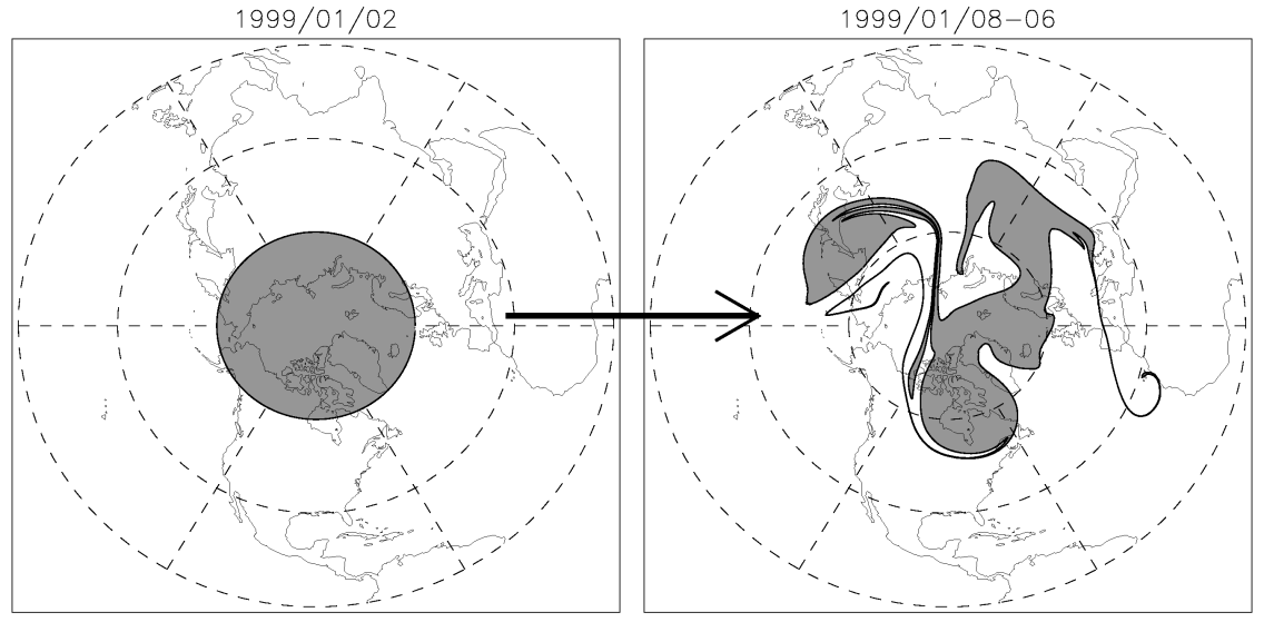
The purpose of this work is to perform contour advection simulations and compare these with isolines of water vapour retrieved from the AMSU-A and -B satellite instruments. While the region of sensitivity of these instruments (the troposphere) means that the contour advection simulations will diverge after a very short period, nonetheless it is hoped that the same fine-scale mixing seen in the simulations will also show up in the retrievals.
2 Data sources
2.1 The AMSU instrument
| channel | centre | sideband | nominal |
|---|---|---|---|
| frequency | offset | width | |
| AMSU-A: | [MHz] | [MHz] | [MHz] |
| 6 | 54400 | 105 | 190 |
| 7 | 54940 | 105 | 190 |
| 8 | 55500 | 87.5 | 155 |
| 9 | 57290 | 87.5 | 155 |
| 10 | 57290 | 217 | 77 |
| AMSU-B: | [GHz] | [GHz] | [GHz] |
| 16 | 89.0 | 0.9 | 1.0 |
| 17 | 159.0 | 0.9 | 1.0 |
| 18 | 183.31 | 1.0 | 0.5 |
| 19 | 183.31 | 3.0 | 1.0 |
| 20 | 183.31 | 7.0 | 2.0 |
| channel | centre | sideband | nominal |
| frequency | offset | width |
AMSU-B is a downward-looking instrument that detects microwave radiation in five double side-band channels in the sub-millimeter range, all sensitive to water-vapour. Three are centred on the water-vapour emission line at 183.31 GHz and two are surface looking, so-called “window” channels, also sensitive to water-vapour and located at 89 and 150 GHz. Since the instrument is a sister to the AMSU-A instrument, the channels are typically numbered between 16 and 20, starting with the two surface looking channels and then the three 183 gigahertz channels, ending with the deepest-looking of the three. (Saunders et al., 1995) Details of all five AMSU-B channels are shown in Table 1 along with a selected sub-set of the AMSU-A channels. (Rosenkranz, 2001; Kramer, 2002) These latter are sensitive to oxygen thus supplying temperature information which is needed for our retrievals. See the Section 2.3 on radiative transfer modelling.
The NOAA series of satellites upon which AMSU is mounted fly in an 833 km sun-synchronous orbit with roughly 14 orbits per day while the instrument uses a cross-track scanning geometry. For AMSU-B, there are 90 different viewing angles between -50 and 50 degrees, sampling at a rate of roughly 22.5 scans per minute. This translates to over 300 000 measurements per satellite per day at resolutions of between 15 and 50 km, while full global coverage requires only a single day of data from three satellites. The AMSU-A instrument has one ninth the resolution as it has only 30 different viewing angles and scans at one-third the rate.
2.2 ECMWF data
The European Centre for Medium-range Weather Forecasting (ECMWF) supplies a synthesized, gridded data set based on an amalgam of in-situ, sonde, satellite and other remote-sensing measurements that have been fitted to a dynamical model, hence the term “assimilation” data. Gridding of the data used in this study is 1.5 by 1.5 degrees longitude and latitude while it is laid out vertically along sixty so-called “sigma” levels. The idea behind sigma levels is that they are terrain following close to the surface but revert to pressure levels at higher altitudes. The pressure at a given ECMWF sigma level is calculated as follows:
| (2) |
where is the level, and are constants and is the surface pressure. For the most comprehensive and up-to-date information on this product, please refer to the ECMWF website: http://www.ecmwf.int/research/ifsdocs/index.html.
Included in the ECMWF data are gridded fields of temperature, pressure, humidity and cloud content, all derived from the ERA-40 product. These will be used both to validate retrievals and to generate the training dataset. For the latter, AMSU radiances are simulated with a radiative transfer model and paired with water-vapour mixing-ratios from the input profiles. The zonal and meridional wind fields will drive the contour advection simulation.
2.3 Radiative transfer modelling
Simulated training data is used instead of actual AMSU measurements co-located with radiosonde measurements for several reasons. First, the irregular coverage of radiosonde launch locations mean that statistics will not be representative. Second, co-locations are never exact in time and space, especially if balloon drift is not accounted for. Moreover, satellite instruments sample a large area while radiosondes will produce point measurements. All these factors will make strictly empirical training data quite noisy, while radiative transfer models have reached a level of maturity that they can accurately model emissions if the atmospheric state is sufficiently well known. In the case of training data, the atmospheric state need not be known exactly anyway; it only has to represent a state that could reasonably occur in the real atmosphere.
For a given vertical profile, the density of radiation at a single frequency emitted to space in a single direction may be modelled via the radiative transfer (RT) equation:
| (3) |
where is the intensity of radiation per solid angle, per unit frequency, is the path (a function of altitude), is the absorption cross-section of the th species, is the density of the th species and is the Planck function. Equation 3 assumes a horizontally isotropic, scattering atmosphere so that is the scattering phase function, which predicts the rate of transfer of radiation from the incoming direction, , to the outgoing direction, , and is the scattering cross-section. The density of the scatterer (here we assume there is only one) is denoted by .
Radiative transfer simulations were performed using RTTOV version 8, a fast radiative transfer simulator. The efficiency of RTTOV is gained by computing a linearized version of the RT equation for emission and absorption while scattering by hydrometeors is treated by the Eddington approximation. (Saunders et al., 2005)
3 Methods
3.1 Contour advection
The evolution of a tracer in Lagrangian coordinates is given very simply as:
| (4) |
where is the concentration of the tracer for a given parcel of air, is time and is the source term. The coordinate evolves according to the transport equation:
| (5) |
where is the velocity of the fluid. Equation (4) assumes that either the fluid is incompressible or the tracer concentration is measured as a mixing-ratio. In what is known as a conserved or passive tracer, there are no source terms and the right-hand-side of (4) will be zero.
In contour advection, only a single isoline is modelled at a time, where:
| (6) |
defines the contour: is the path, is the value of the isoline and is the contour which evolves according to (5). One way to imagine it is to think of a blob of dye injected into a moving fluid. To first order, its evolution may be modelled by considering only its outlines.
It stands to reason that the function, , cannot be represented exactly; naturally, it can be defined to arbitrary precision using a set of discrete points. These are advected by integrating Equation (5), typically with a Runge-Kutta scheme using velocities interpolated from a grid. To maintain a constant precision, new points are added or removed at regular time intervals on the basis of some criterion or metric, either simple distance or curvature as in Dritschel (1988).
We would like each pair of adjacent points to trace out a certain fraction of arc (say, ) so that the curvature criterion may be defined as follows:
| (7) |
where and are the minimum and maximum allowed fractions of arc respectively, is the radius of curvature and is the path difference between two adjacent points. The number of new points added will be in proportion to the ratio of the measure to the maximum, () interpolated at regular intervals along the path.
Parametric fitting of with a cubic spline (Press et al., 1992) will return a set of second order derivatives with respect to the path. These are then used to calculate the curvature so that testing for new points and interpolating them may be done in a single step.
3.2 Adaptive Gaussian filtering
The -nearest neighbours is a popular statistical classification technique in which a fixed number, , of training samples closest to the test point are found and the class determined by voting. (Michie et al., 1994) Consider the following generalization of the scheme:
| (8) | |||||
| (9) |
where is a test point, is a constant, is the class associated with the th sample and is a weight calculated via a filter function:
| (10) |
where is the filter function is its width and is the location in measurement space of the th training sample.
The parameter, , is equivalent to the number of nearest neighbours in a -nearest-neighbours classifier and is held fixed by varying the filter width. This keeps a uniform number of samples within the central region of the filter. An obvious choice for would be a Gaussian:
| (11) |
Where the upright brackets denote a metric, typically Cartesian.
The primary advantage of the above over a -nearest-neighbours, is that it generates estimates that are both continuous and differentiable. Both features may be exploited, first to find the class borders, then to perform classifications and estimate the conditional probability. Let be the difference in conditional probabilities between two classes:
| (12) |
where and are the classes. The border between the two is found by setting this expression to zero. The procedure used was to randomly pick pairs of points that straddle the class border and then solve along the lines between them. Analytical derivatives are used as an aid to root-finding.
The class of a test point is estimated as follows:
| (13) | |||||
| (14) | |||||
| (15) |
where sample the class border and is the retrieved class. The value of may be extrapolated to the test point:
| (16) |
This algorithm is robust, general and efficient, yet still supplies knowledge of the conditional probabilities needed to set a definite confidence limit on the retrieved isoline. It is a variable bandwidth kernel density “balloon” estimator. (Terrell and Scott, 1992)
Mills (2011) provides a more thorough description of the AGF algorithm.
3.3 Isoline retrieval

For performing classifications of water-vapour mixing-ratio for the purpose of isoline retrieval, the vector was defined as follows:
| (17) |
where is the brightness temperature of the th AMSU channel and is its corresponding standard deviation. The first four coordinates supply temperature information, while the last three supply the humidity information. All seven have weighting functions–defined as the gradient of the brightness temperature with respect to changes in water-vapour at each vertical level–that peak in the troposphere with relatively little surface contribution on average, especially in the lower latitudes where the air is moist.
The classes are defined as follows:
| (18) |
where is the class, is mass-mixing-ratio of water vapour (specific humidity) and is the isoline we are trying to retrieve.
To supply the training data, 86 000 profiles were randomly selected in both time and space from the ECMWF data. Radiative transfer simulations were performed using RTTOV, including both scattering and clouds, to generate the brightness temperatures needed in (17). For ice cloud simulations, we used aggregrate crystal shapes having a size distribution as described in Wyser (1997). This training data will also be used for the actual retrievals.
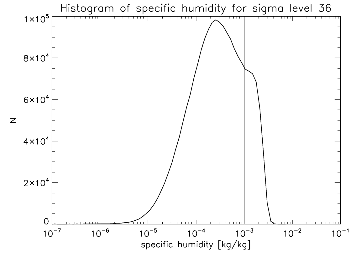
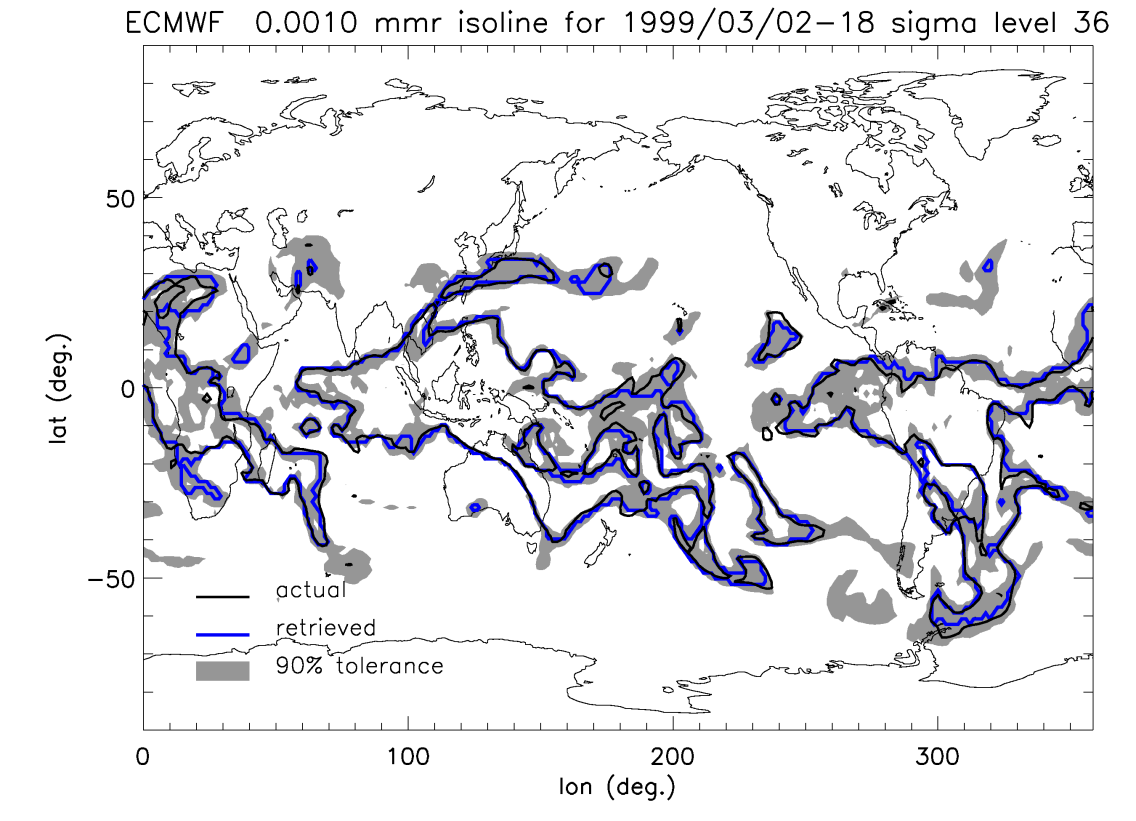
The retrieval was performed along ECWMF sigma level #36 (approx. 400 hPa) since this is roughly in the centre of the region of sensitivity for the seven channels. Retrievals performed on isentropic surfaces are not accurate because altitude tends to increase with latitude while the instrument weighting functions do the opposite. To determine the threshold value for water-vapour, we first look at the statistics, as shown in Figure 2. Note the extended tail, with the discontinuity ( mass-mixing-ratio) being the best threshold. Selecting the threshold in the valley between the peaks of a bi-modal (or in this case, almost bi-modal) distribution should reduce the error rate because the continuum value is more likely to occur near one of the two peaks, away from the threshold.
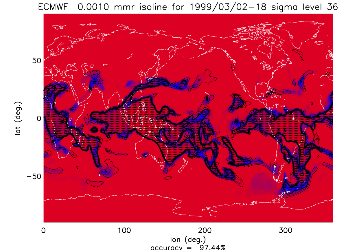
Once classifications have been done over a large enough section of the Earth’s surface, isolines are retrieved by simply tracing the borders between positive (higher than the threshold) and negative (lower than the threshold) classification results via any contouring algorithm. The results of a simulated test retrieval are shown in Figure 3 using the aforementioned training data. To compute the test data, additional radiances were calculated from a global ECMWF field in the same manner as for the training data. To account for differences in surface emissivity, the test data was divided into land and sea and retrieved using two, separately simulated sets of training data.
The heavy black line in Figure 3 is the “true” isoline, with auxiliary fine contours for higher and lower multiples. The retrieved isoline is not shown; rather a dot indicates a positive classification. Obviously, all the dots should fall within the heavy contour, but like a young child who has not yet learned how to colour, the retrieval does not perfectly fill the isoline.
The shading indicates the confidence rating which we define by simply rescaling the conditional probability:
| (19) |
where is the winning class and is the number of classes. If C is zero, then the classification result is little better than chance, while if one then it should be perfect, assuming that the conditional probability has been estimated accurately.
As might be expected, the confidence is lower closer to the isoline, as well as where the gradients are shallow. The measure may be used to define an interval within which the true isoline is likely to fall: a “cutoff” value is chosen and the area thus enclosed will contain the true isoline to within a certain statistical tolerance.
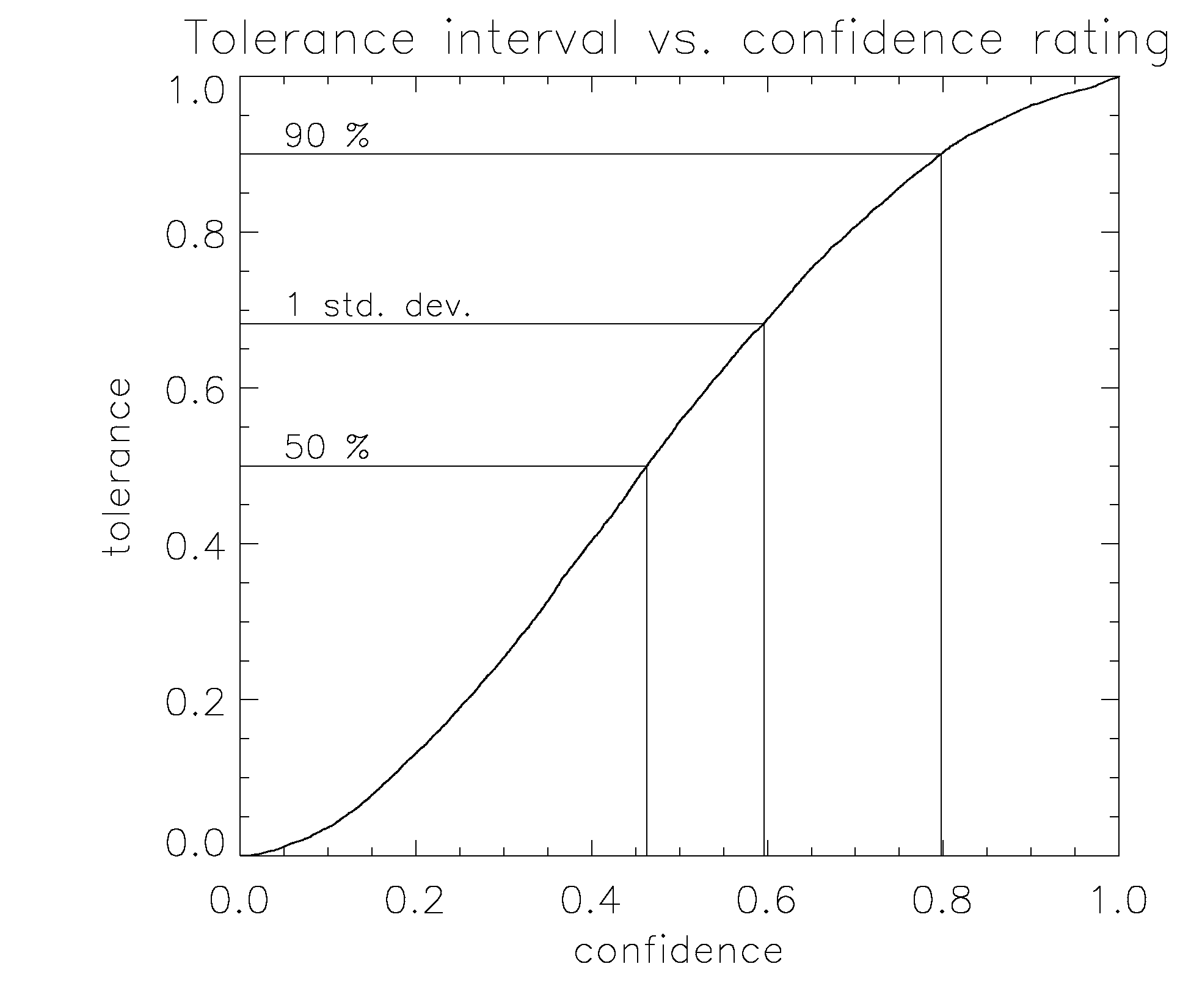
To calculate the tolerance from the confidence rating, a rather tedious line-integral method was used, expressed mathematically as follows:
| (20) |
where is the Heaviside function, is the tolerance of the retrieved isoline as a function of confidence rating and is the confidence rating of the classification results as a function of geographical position, . The integral is performed along the length, , of the actual isoline. Although (20) implies that the integral must be evaluated separately for each value of the confidence rating, , in actual fact it may be done for all values of by sorting the confidence ratings of the results, i.e., .
Figure 4 plots the combined results of Equation (20) for six (6) different simulated retrievals. Fifty percent, ninety percent and one-standard deviation (assuming the statistics are Gaussian) intervals are indicated in the figure. This result will be used for the actual retrievals and in Figure 5 which, while containing nothing that Figure 3 does not, demonstrates how to set a definite tolerance limit on the retrieved isoline. Now the solid line represents the true isoline which we expect to fall within the shading ninety percent of the time, while the broken line is the retrieval.
4 Results
Since the AMSU instrument views the Earth at many different angles to produce a swath, several sets of training data corresponding to some or all of these viewing angles must be employed to perform actual retrievals. Radiative transfer simulations were performed at sixteen different angles, one at nadir and one for every third angle of the ‘B’ instrument along one side of the track. Results are interpolated for intermediate angles.
Retrievals were performed at the resolution of AMSU-B by interpolating the AMSU-A data to its equivalent. Since the ‘A’ instrument detects temperature which has a diffusion mechanism (radiative transfer) not available to other tracers, we expect the small-scale variations to be less pronounced. Therefore, the final resolution should be closer to that of the ‘B’ instrument.
4.1 Interpolation
Before generating the contours for both the isoline and the confidence interval, evenly gridded values must be produced at fixed times. Since the satellite data is not as irregular as it first seems, interpolates can be calculated using a simple modification of the multi-linear method. Scan tracks generate samples along a grid that is rectangular to good approximation, therefore we search both forward and backward in time for the two nearest swaths having at least four samples that spatially enclose the interpolation point. Bilinear interpolation is performed for both times and the final result linearly interpolated between these two values.
A more accurate result could be obtained by accounting for the motion of the air parcel, but since we are trying to validate a simulation based on wind circulation, this would obviously contaminate the results.
Conditional probabilities have been derived for a specific humidity (mass-mixing-ratio) threshold of 0.001 for each measurement pixel over a nine-day period from 1 September 2002 to 9 September 2002. These in turn were interpolated to a rectangular lon-lat grid with a resolution of 0.2 degrees at twelve-hour intervals over a period of five days starting at the third of September. The two-day overshoot in the initial time interval is necessary for the interpolation procedure. The maximum interval between adjacent swaths ahead of and behind the interpolation times was slightly over two days, while the average was roughly six hours.
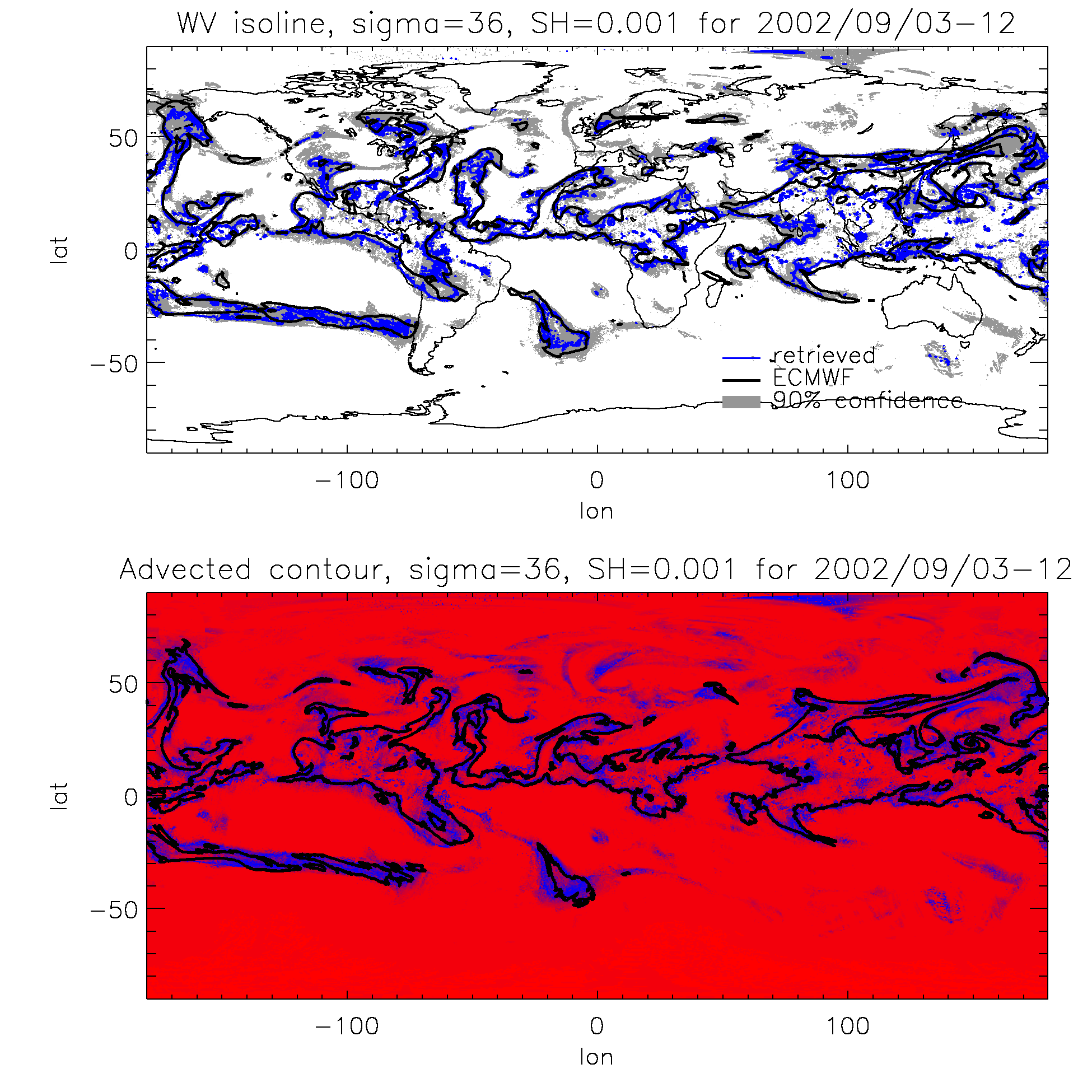
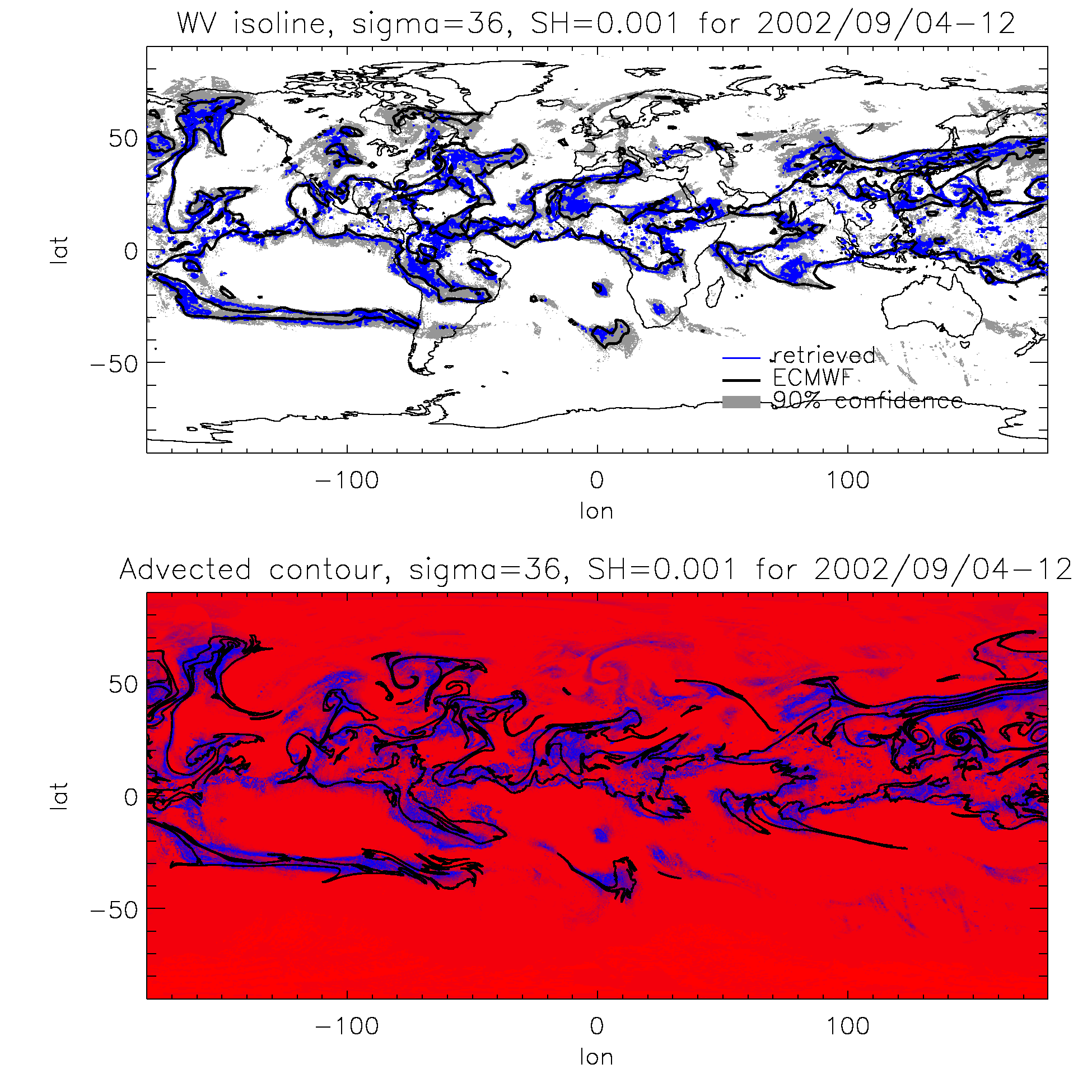
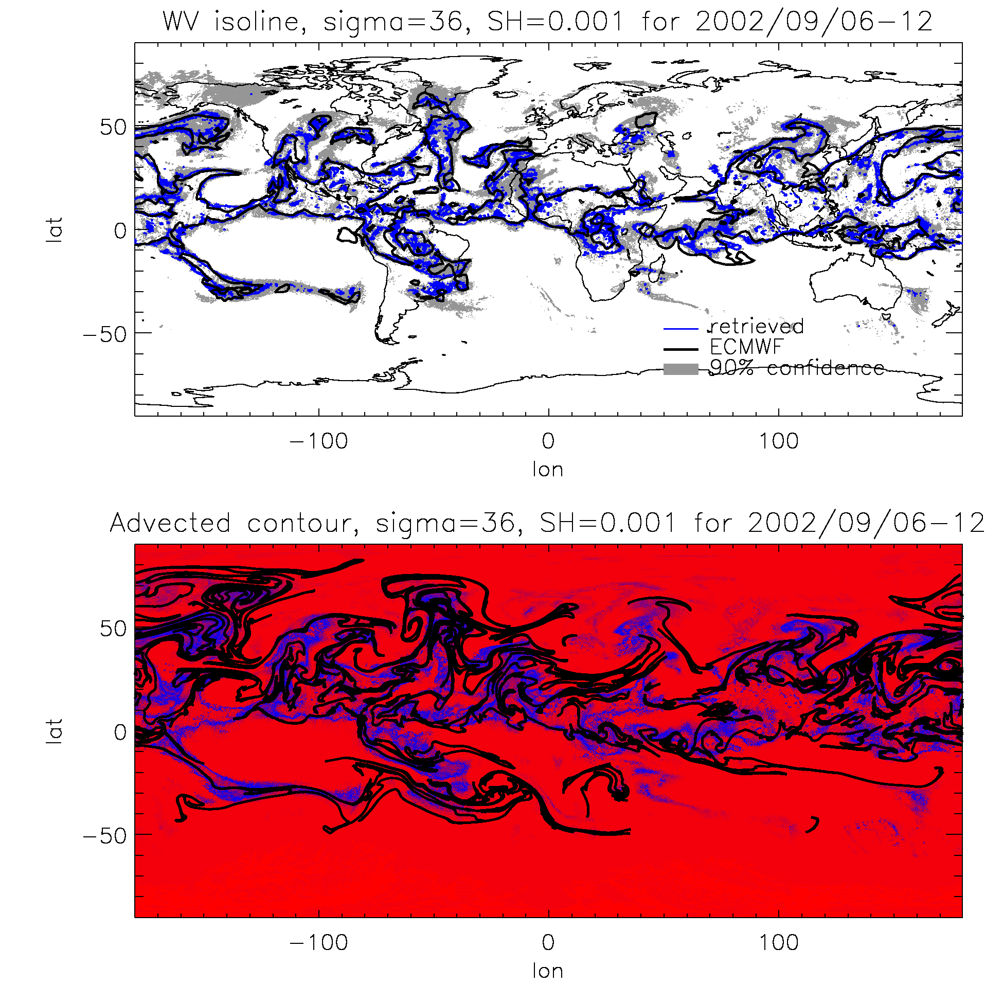
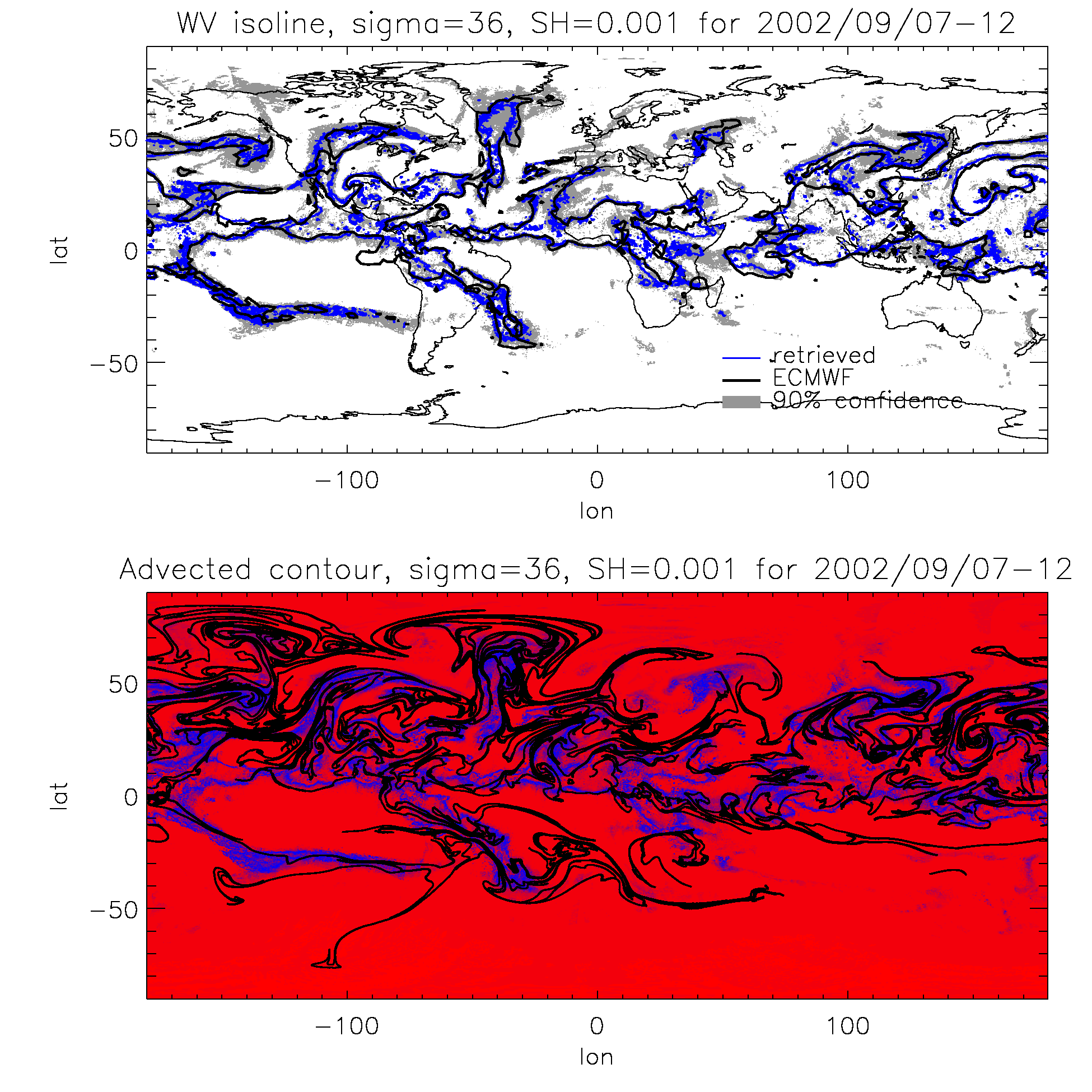
The results for the 12 hour retrievals are shown in Figures 11 through 15. The top of each plot displays the retrieval versus the ECMWF isoline with the grey shading enclosing the 90% tolerance while the bottom shows the advected contours with the differential shading indicating the confidence rating. Contours were advected using 4 Runge-Kutta steps every six hours after which the they were re-interpolated so that each pair of points traced out a minimum fraction of arc of 0.5 degrees and a maximum of one degree. Contours were initialised with isoline retrievals from the 3 September, 00 UTH.
4.2 Calibration and validation
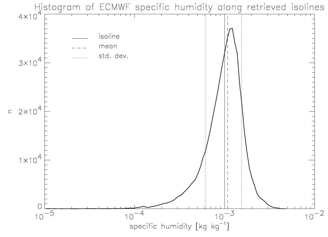
The distribution of ECMWF specific humidity values along the retrieved isolines is shown in Figure 6. The bias is while the standard deviation is .
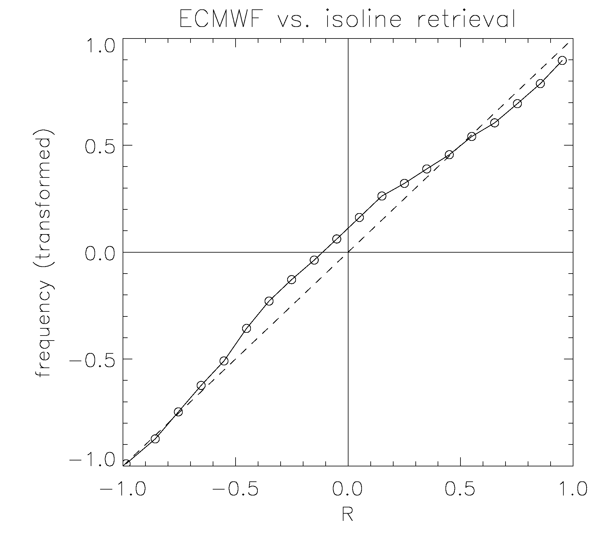
Retrieved conditional probabilities were also validated against the ECMWF data by comparing them with the class frequency. The conditional probabilities were binned at even intervals and an average taken. The relative accuracy or frequency for each bin was then computed for the corresponding ECMWF-derived classifications and plotted with respect to the former as shown in Figure 7.
| threshold | accuracy | ||
|---|---|---|---|
| value of R | class 1 | class 2 | overall |
| -1.0 | 0.001 | 1.00 | 0.238 |
| -0.9 | 0.821 | 0.976 | 0.844 |
| -0.8 | 0.879 | 0.953 | 0.890 |
| -0.7 | 0.907 | 0.930 | 0.910 |
| -0.6 | 0.925 | 0.906 | 0.922 |
| -0.5 | 0.937 | 0.882 | 0.929 |
| -0.4 | 0.947 | 0.856 | 0.933 |
| -0.3 | 0.954 | 0.828 | 0.936 |
| -0.2 | 0.961 | 0.800 | 0.937 |
| -0.1 | 0.966 | 0.771 | 0.937 |
| 0.0 | 0.971 | 0.741 | 0.937 |
| 0.1 | 0.975 | 0.709 | 0.936 |
| 0.2 | 0.978 | 0.675 | 0.933 |
| 0.3 | 0.981 | 0.638 | 0.931 |
| 0.4 | 0.984 | 0.597 | 0.927 |
| 0.5 | 0.987 | 0.552 | 0.923 |
| 0.6 | 0.990 | 0.498 | 0.918 |
| 0.7 | 0.993 | 0.434 | 0.916 |
| 0.8 | 0.995 | 0.350 | 0.900 |
| 0.9 | 0.998 | 0.225 | 0.884 |
| 1.0 | 1.00 | 0.000 | 0.853 |
When considered strictly in terms of the conditional probabilities, it becomes possible to make the retrievals essentially perfect by re-scaling the probabilities to match actual frequencies. (Jolliffe and Stephenson, 2003) Visual inspection of the retrievals suggests a dry bias in comparison to the ECMWF, as the retrieved isolines usually fall inside (on the high humidity side) of the ECMWF contours. This is confirmed in the plot as the actual frequency is higher at the probability corresponding to the isoline (). Table 2 shows the effect on classification accuracy relative to the ECMWF of rescaling the value of at , i.e. at the class border.
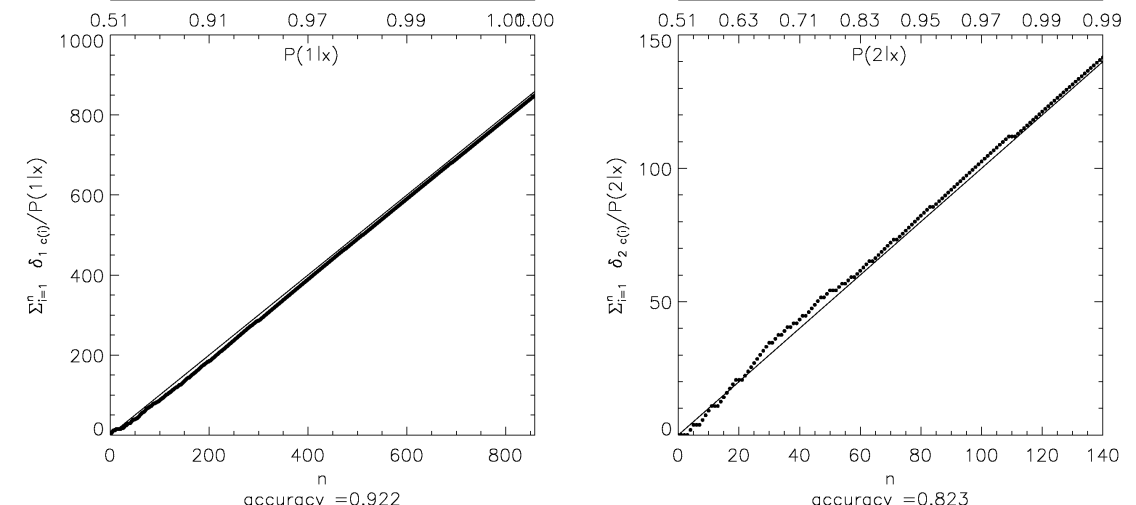
The conditional probabilities were similarly validated relative to radiosonde measurements. Since there were not enough measurement points to generate reliable statistics by binning, an integral method was used. From Bayes’ theorem:
| (21) |
where is the number of classes with value . Transforming this into a Monte Carlo sum:
| (22) |
where is the satellite measurement vector at measurement point . The relationship should hold regardless of the particular choice of points. By sorting the probabilities and then comparing their cumulative sum with the number of classes, we gain an idea of the relative bias at each value.
This will generate a distorted graph, however: points at the beginning of the trace will be much more closely spaced than those toward the end. Therefore, we rearrange Equation (22) as follows:
| (23) |
where is the Kronecker delta and is the “true” class (derived from radiosonde measurements) at point . Now the cumulative sum will follow, on average, one-step intervals between each point in the analysis. To prevent singularities at low values of the conditional probabilities, the analysis was done separately for each class in the retrievals, as shown in Figure 8. 1001 launches from 215 stations–primarily in the Northern Hemisphere–were used in the analyis. The plots deviate very little from the diagonal, implying that there is little bias relative to the radiosonde measurements. Overall classification accuracy was 90.8%. The location error in the radiosonde measurements is one factor limiting the accuracy of these comparisons since balloon drift has not been accounted for.
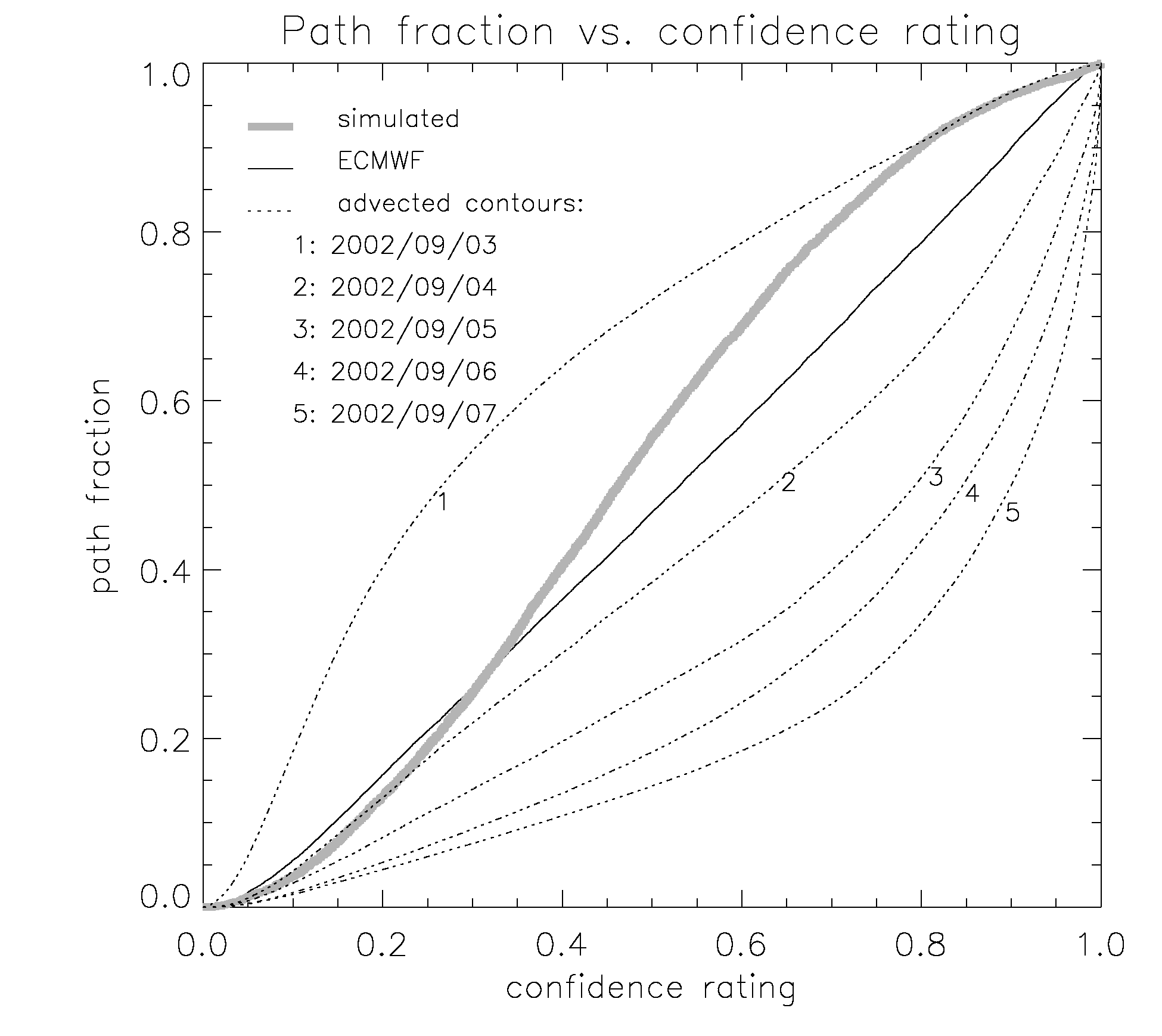
Finally, the retrievals were validated by applying the line integral in (20) to both the ECMWF isolines and to the advected contours using the retrieved confidence ratings. These are compared in Figure 9 to the same function, first presented in Figure 4, derived from simulated retrievals. While the ECMWF isolines were integrated for the entire span of five days, the advected contours were integrated day by day for both the 0 hr and 12 hr retrievals to see the change in accuracy over time.
The confidence rating will approach zero along the isoline, thus the more closely the reference isoline matches the retrieved, the further up and to the left the function will be, with an exact match returning the Heaviside function. The thick, grey line from the simulation runs provides an upper limit to retrieval accuracy: any new sources of error, either in the retrieval or in the reference, will move the integral down and to the right. Since advected contours were initialised with retrieved isolines, the very first ones lie to the left.
5 Discussion

The study of chaotic mixing is interesting, not only in its own right, but also for its potential to improve fluid modelling in geophysical systems. It is particularly relevant to the parameterisation of large-scale diffusion in circulation models, since mechanical stirring enhances diffusion. (Nakamura, 2001; Thiffeault, 2003) A unique approach to this phenomenon is the modified Lagrangian mean formalism by Nakamura (1998). A set of retrieved contours would lend themselves well to this type of analysis.
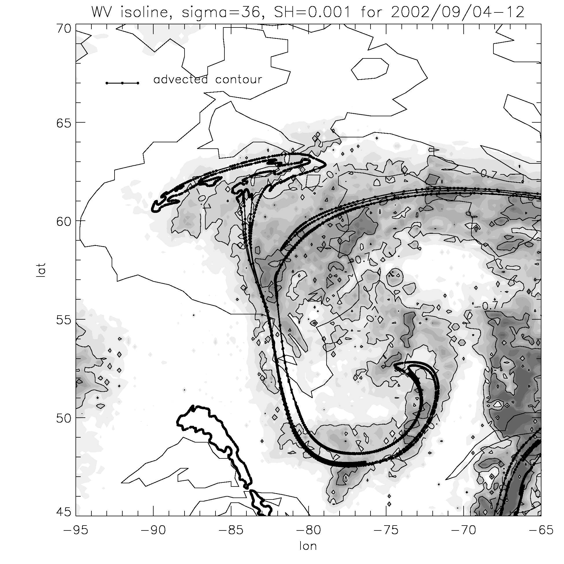
But first we must answer the question addressed by this paper: is there evidence of chaotic mixing in the satellite data? Looking strictly at the isoline retrievals proper, the answer is, “no.” Evidence of fine-scale mixing is, however, apparent in the conditional probabilities. Many of the filaments seen in the advected contours also show up as traces of reduced “confidence rating.” In other words, there is a non-negligible probability (less than 50 %) that the filament might be there. Recalling how the retrieval may be recalibrated: by changing the threshold value of R at which the isoline is drawn, the filaments are thereby exposed with relatively little effect on the larger “islands.” See for example the expanded detail of the anticyclone in the North-West corner of the 4 September retrieval (Figure 12) in Figure 10.
There are a number of difficulties and sources of error associated with this study. The advected contours especially are of limited accuracy, even over short time scales and they diverge rapidly. Contours are advected on sigma levels and do not take into account non-adiabatic vertical motion, which can be strong in the troposphere. The choice of sigma levels over isentropic levels had more to do with retrieval accuracy but further reduces the effectiveness of the transport model, since even adiabatic motion in the vertical is now neglected. Another limitation of contour advection is that it cannot easily account for sources or sinks which are numerous for water-vapour. The high value chosen, while making detection easier, will bring with it a high occurrence of clouds and precipitiation. There is a further sense in which water-vapour is not a “passive” tracer: it will affect the motion. Repeating the analysis with a similar instrument that detects ozone in the stratosphere, such as GOME, would likely produce more satisfying results.
The retrieval method suffers from similar limitations. In particular, it attempts to limit the retrieval to a single vertical level, a feat that is difficult to accomplish with only seven channels to work with. This is the main reason why the retrievals are seen to have such a broad tolerance interval. Another difficulty is the scattering generated by clouds, which for high, thick cover may interfere with the view of the target level. Adding the two lowest frequency AMSU-B channels might help address both issues, but this requires accurate knowledge of the surface emissivities.
Finally, some minor artifacts are produced by the interpolation procedure at junctions between scan lines. These could be cleaned up by some sort of image processing technique, such as filtering. Interpolation could also be done at narrow time intervals and additional filtering applied in the time domain so as to include extra measurement pixels in each grid point.
These and other difficulties only serve to underline the considerable potential of the inversion method. Producing continuum retrievals, for instance, would be a trivial extension accomplished by generating several contours and interpolating between them. Since satellite retrievals are rarely better than 5 % accurate, the error produced by interpolation would be negligible in comparison. It would follow that generating continuum values from a two-dimensional array of discrete ones would be more effective than relying solely on individual pixels. An accurate characterisation of the error at each point in the field is easily generated as a by-product from the combination of confidence ratings and tracer gradients.
6 Conclusion
The natural apex of satellite remote sensing is that of an intimate, real-time picture of the atmosphere down to the finest detail. Neural networks, statistical classification and similar machine learning techniques provide a nice alternative to complex inverse methods such as optimal estimation that use forward models directly. As the models become more detailed and precise, it becomes increasingly difficult to apply the latter methods with anything resembling analytical precision. Machine learning techniques, by contrast, easily generate an inverse model that can be applied directly and efficiently to the data. Although it is usually impossible to derive analytical inverse functions for complex radiative transfer models, there is no reason that a numerically generated one not be used instead. While the current paper does use an involved forward model to generate the training data, as the satellite record becomes longer, this can be superceded by satellite measurements paired with co-located, direct measurements, obviating the need for lengthy simulations runs, while ensuring accuracy.
In this paper we have generated very specific retrievals that detect from high-resolution AMSU satellite measurements only a single isoline of water-vapour along a single vertical level in the upper troposphere. These retrievals were shown to have good agreement both with ECMWF assimilation data and with radiosonde measurements. The method is shown to have excellent potential for detecting fine-scale features produced by chaotic mixing, although this is hampered by the poor vertical resolution of the instrument, resulting in reduced accuracy which in turn decreases the effective horizontal resolution.





Acknowledgements
Thanks very much to my colleagues and supervisors (both present and former) from the IUP for encouraging and supporting this work, Georg Heygster and Stefan Buehler in particular. Thanks to Stefan, Mashrab Kuvatov and Christian Melsheimer for very valued comments on the draft manuscript.
Thanks to ECMWF for ERA 40 data, to the RTTOV development team at the UK met office, to the Danish Meteorological Institute for the database of compiled radio soundings and to Lisa Neclos from the Comprehensive Large Array-data Stewardship System (CLASS) of the US National Oceanic and Atmospheric Administration (NOAA) for AMSU data.
Appendix A Proof of increased accuracy
Suppose we have a conditional probability, describing the distribution of states, , for a given measurement variable, . Discretizing the problem into only two states, with the threshold given by , the continuum distribution transforms as follows:
| (24) | |||
| (25) |
If only these discrete states are required, it is very easy to show that a classification retrieval will be more accurate than one over a continuum. The accuracy of a series of classification results over an area, , is given as follows:
| (26) |
where is the class as an integer function of position. Full knowledge of the conditional probability is assumed. The value of this integral takes on a maximum when the integrand is maximised at each point:
| (27) |
Since this is simply the definition of maximum likelihood, it is apparent that any other method of selecting the class will produce less accurate results.
Continuum retrievals are generally performed by taking an expectation value:
| (28) |
where is the state variable and the retrieved state variable. In the continuum case, the class, , is selected quite as follows:
| (29) |
This will produce different results than a maximum likelihood classification.
References
- Appenzeller et al. (1996) Appenzeller, C., Davies, H., and Norton, W. (1996). Fragmentation of stratospheric intrusion. Journal of Geophysical Research, 101(D1):1435–1456.
- Dritschel (1988) Dritschel, D. G. (1988). Contour surgery: A topological reconnection scheme for extended integrations using contour dynamics. Journal of Computational Physics, 77:240–266.
- Dritschel (1989) Dritschel, D. G. (1989). Contour dynamics and contour surgery: Numerical algorithms for extended, high-resolution modelling of vortex dynamics in two-dimensional, inviscid, incompressible flows. Computer Physics Reports, 10:77–146.
- Jolliffe and Stephenson (2003) Jolliffe, I. and Stephenson, D. (2003). Forecast Verification: A Practitioner’s Guide in the Atmospheric Sciences. John Wiley and Sons, Somerset, NJ.
- Kramer (2002) Kramer, H. J. (2002). Observations of Earth and Its Environment: Survey of Missions and Sensors. Springer-Verlag, New York.
- Methven and Hoskins (1999) Methven, J. and Hoskins, B. (1999). The advection of high-resolution tracers by low-resolution winds. Journal of the Atmospheric Sciences, 56(18):3262–3285.
- Michie et al. (1994) Michie, D., Spiegelhalter, D. J., and Tayler, C. C., editors (1994). Machine Learning, Neural and Statistical Classification. Ellis Horwood Series in Artificial Intelligence. Prentice Hall, Upper Saddle River, NJ.
- Mills (2011) Mills, P. (2011). Efficient statistical classification of satellite measurements. International Journal of Remote Sensing, 32(21):6109–6132.
- Nakamura (1998) Nakamura, N. (1998). Leaky containment vessels of air: a lagrangian mean approach to the stratospheric tracer transport. In Singh, M. P. and Raman, S., editors, Advances in Fluid Mechanics: Dynamics of Atmospheric Flows. Part I, Atmospheric Transport and Diffusion Processes, pages 193–246. Computational Mechanics Publications, Ashurst Lodge, UK.
- Nakamura (2001) Nakamura, N. (2001). A new look at eddy diffusivity as a mixing diagnostic. Journal of Atmospheric Sciences, 58:3686–3701.
- Ott (1993) Ott, E. (1993). Chaos in Dynamical Systems. Cambridge University Press, Cambridge, UK.
- Ottino (1989) Ottino, J. M. (1989). The Kinematics of Mixing: stretching, chaos and transport. Cambridge University Press, Cambridge, UK.
- Press et al. (1992) Press, W. H., Teukolsky, S. A., Vetterling, W. T., and Flannery, B. P. (1992). Numerical Recipes in C. Cambridge University Press, Cambridge, UK, second edition.
- Rodgers (2000) Rodgers, C. D. (2000). Inverse Methods for Atmospheric Sounding: Theory and Practice. World Scientific, London.
- Rosenkranz (2001) Rosenkranz, P. W. (2001). Retrieval of temperature and moisture profiles from AMSU-A and AMSU-B measurements. IEEE Transactions on Geoscience and Remote Sensing, 39(11):2429–2435.
- Saunders et al. (2005) Saunders, R., Brunel, P., Bauer, P., O’Keeffe, U., Francis, P., and Rayer, P. (2005). RTTOV-8 science and validation report. Technical report, EUMETSAT, The Met Office, UK.
- Saunders et al. (1995) Saunders, R. W., Hewson, T. J., Stringer, S. J., and Atkinson, N. C. (1995). The radiometric characterization of AMSU-B. IEEE Transactions on Microwave Theory and Techniques, 43:760–771.
- Terrell and Scott (1992) Terrell, D. G. and Scott, D. W. (1992). Variable kernel density estimation. Annals of Statistics, 20:1236–1265.
- Thiffeault (2003) Thiffeault, J. L. (2003). Advection-diffusion in Lagrangian coordinates. Physics Letters A, 309:415–422.
- Waugh and Plumb (1994) Waugh, D. W. and Plumb, R. A. (1994). Contour advection with surgery: a technique for investigating fine scale structure in tracer transport. Journal of the Atmospheric Sciences, 51(4):530–540.
- Wyser (1997) Wyser, K. (1997). The Effective Radius of Ice Clouds. Journal of Climate, 11:1793–1802.