Periodic-orbit approach to the nuclear shell structures with power-law potential models:
Bridge orbits and prolate-oblate asymmetry

Abstract

Deformed shell structures in nuclear mean-field potentials are systematically investigated as functions of deformation and surface diffuseness. As the mean-field model to investigate nuclear shell structures in a wide range of mass numbers, we propose the radial power-law potential model, $V\propto r^{\alpha}$, which enables us a simple semiclassical analysis by the use of its scaling property. We find that remarkable shell structures emerge at certain combinations of deformation and diffuseness parameters, and they are closely related to the periodic-orbit bifurcations. In particular, significant roles of the “bridge orbit bifurcations” for normal and superdeformed shell structures are pointed out. It is shown that the prolate-oblate asymmetry in deformed shell structures is clearly understood from the contribution of the bridge orbit to the semiclassical level density. The roles of bridge orbit bifurcations in the emergence of superdeformed shell structures are also discussed.

I Introduction

Shell structures in single-particle energy spectra play essential roles in nuclear ground-state deformations and their stabilities. Using the semiclassical trace formula, single-particle level density is expressed as the sum over contributions of classical periodic orbits in the corresponding classical Hamiltonian systemGutz ; BaBlo . The quantum fluctuations in many-body quantities such as energy and deformations are related to gross shell structure in single-particle spectra determined by some short periodic orbits. Therefore, one can describe many-body quantum dynamics in terms of the properties of a few important classical periodic orbits. The single-particle shell structures are sensitively affected by varying potential parameters such as deformations, and we have found that bifurcations of short periodic orbits play significant roles in emergence of remarkable shell effects. It is a quite interesting phenomena that the regularity of quantum spectra is enhanced by the periodic-orbit bifurcation, which is regarded as the precursor of chaos in classical dynamics. In this paper, we would like to show that the above semiclassical mechanism for the enhancement of quantum shell effects would elucidate several problems in nuclear structure physics.

As phenomenological mean-field potentials, modified oscillator (MO) and Woods-Saxon (WS) models are successfully employed in shell correction approaches. For simpler and qualitative descriptions of the properties of shell structures, harmonic oscillator (HO) and infinite-well (cavity) potentials are frequently utilized for light and heavy systems, respectively. Axially symmetric anisotropic HO potential models successfully explain the magic numbers of light nuclei, emergence of superdeformed shell structures, and so on. For heavier nuclei, the radial profile of the potential around the nuclear surface becomes more sharp and it looks more like a square-well potential. In order to avoid the complexity of treating continuum states, the WS potential is sometimes approximated by an infinite-well potential (cavity). The cavity system, as well as the HO system, is integrable under spheroidal deformation due to the existence of a nontrivial dynamical symmetry, and several classical and quantum mechanical quantities are obtained analytically. It also accepts several useful techniques to calculate quantum eigenvalue spectra, since the Schrödinger equation is equivalent to the Laplace equation with Dirichlet boundary condition.

The HO and cavity systems have a significant difference in deformed shell structures. In the axially-deformed HO system, the ways in which the degeneracy of levels is resolved, due to prolate and oblate deformations, are nearly symmetric; namely, the level diagram vs deformation is symmetric under rotation about the degenerate spherical point by angle $\pi$. Due to this symmetry, many-body systems between adjacent closed-shell configurations will prefer prolate shapes in the lower half shell and oblate shapes in the higher half shell, since single-particle level density is lower there, and in total, prolate and oblate shapes are expected to occur in almost the same ratios. On the other hand, the above kind of symmetry is apparently broken in the cavity system. Such asymmetry has been considered as the origin of so called prolate-shape dominance in nuclear ground-state deformations: a well known experimental fact that most of the ground states of medium-mass to heavy nuclei have prolate shapes rather than oblate shapes. Its origin has been discussed since the discovery of the nuclear ground-state deformationBM_II ; Tajima96 ; Tajima2001 ; Takahara . This predominance has been reproduced theoretically in microscopic calculations. In Hartree-Fock+BCS calculations with Skyrme interactionTajima96 , most of the deformed ground-state solutions are found to have prolate shapes. In order to pin down the essential parameter which causes prolate-shape dominance, systematic Nilsson-Strutinsky calculations throughout the nuclear chart have been madeTajima2001 , and the distribution of ground-state deformations is examined by varying the strengths of $l^{2}$ and $ls$ terms in the Nilsson Hamiltonian. They found that the prolate-shape dominance is realized under strong correlation between $l^{2}$ and $ls$ terms. The recent analysis by Takahara et al. based on Woods-Saxon-Strutinsky calculations also supports those resultsTakahara . Hamamoto and Mottelson compared the oblate and prolate deformation energy from the summation of single-particle energies with spheroidal HO and cavity models, and have shown that the prolate-shape dominance is only found in the cavity model. They considered the origin of the prolate-shape dominance to be the asymmetric manner of level fannings in prolate and oblate sides which is unique to a potential with a sharp surface, and have shown that the above asymmetry is explained from the different roles of interaction between single-particle levels in prolate and oblate sidesHamMot .

We expect that the semiclassical periodic-orbit theory (POT) holds the key for deeper understandings of above shell structures responsible for prolate-shape dominance. In POT, semiclassical level density is expressed as the sum of periodic orbit (PO) contributions,

$$g(E)=\bar{g}(E)+\sum_{\beta}A_{\beta}(E)\cos\left(\frac{S_{\beta}(E)}{\hbar}-\frac{\pi\mu_{\beta}}{2}\right).$$ (1)

$\bar{g}$ is the average level density equivalent to that given by the Thomas-Fermi approximation, and the second term on the right-hand side gives the fluctuations around $\bar{g}$. The sum is taken over all the classical periodic orbits $\beta$ which exist for given energy $E$. $S_{\beta}=\oint_{\beta}\mathbi{p}\cdot d\mathbi{r}$ is the action integral, and $\mu_{\beta}$ is the geometric phase index determined by the number of conjugate points along the orbit. Each orbit $\beta$ changes its size and shape with increasing energy $E$, and the action integral $S_{\beta}$ is, in general, a monotonically increasing function of $E$. Thus, each cosine term in the PO sum (1) is a regularly oscillating function of energy whose period of oscillation $\delta E$ is given through the relation

$$\delta S_{\beta}\sim\frac{\partial S_{\beta}}{\partial E}\delta E\sim 2\pi\hbar,\quad\delta E\sim\frac{2\pi\hbar}{T_{\beta}},$$ (2)

where $T_{\beta}=\partial S_{\beta}/\partial E$ is time period of the orbit $\beta$. Therefore, a gross shell structure (large $\delta E$) is associated with short periodic orbits (small $T_{\beta}$).

The above fluctuation in the single-particle spectrum brings about a fluctuation in energy of nuclei as functions of constituent nucleon numbers. This fluctuation part, which we call shell energy, is calculated by removing the smooth part from a sum of single-particle energies by means of the Strutinsky methodStrut ; BrackPauli . In semiclassical theory, shell energy $E_{\rm sh}(N)$ is given by the sum of periodic orbit contribution asBBText

$$E_{\rm sh}(N)=\sum_{\beta}\left(\frac{\hbar}{T_{\beta}}\right)^{2}A_{\beta}\cos\left(\frac{S_{\beta}(E_{F}(N))}{\hbar}-\frac{\pi\mu_{\beta}}{2}\right),$$ (3)

where the Fermi energy $E_{F}(N)$ is determined by

$$\int_{-\infty}^{E_{F}}g(E)dE=N.$$ (4)

In Eq. (3), the contributions of long orbits are suppressed by the reduction factor $T_{\beta}^{-2}$, and the property of shell energy is essentially determined by a few shortest periodic orbits. Therefore, it is sufficient to examine coarse-grained level density where one can exclude the contribution of long periodic orbits.

The relation between coarse-grained quantum level density oscillations and classical periodic orbits in the spherical cavity model was first discussed by Balian and BlochBaBlo . They show that the modulations in quantum level density oscillations are clearly understood as the interference effect of periodic orbits with different lengths. This idea has been successfully applied to the problem of supershell structure in metallic clustersNishioka . Strutinsky et al.StrMag applied periodic orbit theory (POT)Gutz ; BaBlo to the cavity model with spheroidal deformation and discussed the properties of deformed shell structures in medium-mass to heavy nuclei in terms of classical periodic orbitsStrMag . Frisk made more extensive POT calculations to reproduce quantum level density by the semiclassical formulaFrisk . He also suggested the relation between classical periodic orbits and prolate-oblate asymmetry in deformed shell structures, which might be responsible for the prolate-shape dominance discussed above. Those works have proved the virtue of semiclassical POT for clear understanding of the properties of finite quantum systems.

It should be emphasized here that unique deformed shell structures are developed when the contributions of certain periodic orbits are considerably enhanced. The magnitude of the shell effect is related to the amplitude factor $A_{\beta}$ in Eq. (1). This amplitude factor has important dependency on the stability of the orbit, which is generally very sensitive to the potential parameters such as deformations. In particular, stability factors sometimes exhibit significant enhancement at periodic orbit bifurcations, where new periodic orbits emerge from an existing periodic orbit. Near the bifurcation point, classical orbits surrounding the stable periodic orbit form a quasiperiodic family, which makes a coherent contribution to the level density. This is an important mechanism for the growth of deformed shell structures.

A typical example is the so-called superdeformed shell structure. It is known that single-particle spectra exhibit remarkable shell effects at very large quadrupole-type deformation with an axis ratio around 2:1. In the anisotropic HO model, this shell structure is related with the periodic orbit condition; all the classical orbits become periodic at $\omega_{\perp}=2\omega_{z}$ and they make very large contribution to the level density fluctuation. In the cavity model, one also finds a significant shell effect around the 2:1 deformation, and it is related to the bifurcations of equatorial periodic orbits through which three-dimensional (3D) periodic orbits emergeASM ; Magner2 . It should be interesting to explore the intermediate situation between the above two limits, which might correspond to the actual nuclear situation.

Our purpose in this paper is to understand the transition of deformed shell structure from light to heavy nuclei in terms of classical periodic orbits. This requires a mean field like WS potential model. Semiclassical quantizations in spherical and deformed WS-like potentials have been examined in Refs. Carb ; Arv , but the relation between classical periodic orbits and quantum level densities has not been discussed. As we show, the WS potential inside the nuclear radius $R_{A}$ is nicely approximated by a power-law potential which has simpler radial dependence $V\propto r^{\alpha}$. This approximation simplifies both quantum and classical calculations and one has clear quantum-classical correspondence via the Fourier transformation techniqueIJMPE .

Thus, in the current paper, we focus on the radial dependence of the mean-field potential (effect of surface diffuseness, described by the $l^{2}$ term in the Nilsson model) and examine the shell structures systematically as functions of deformation and surface diffuseness. As pointed out by Tajima et al., spin-orbit coupling plays also an important role in prolate-shape dominance. The effect of spin-orbit coupling will be discussed in a forthcoming paper.

This paper is organized as follows. In Sec. II, we discuss the quantum and classical properties of the power-law potential model. The scaling properties of the model are described and the Fourier transformation techniques are formulated. In Sect. III, quantum mechanical densities of states and shell structures in the spherical power-law potential are examined. Some analytic expressions for periodic orbit bifurcations and semiclassical formulas are given, and quantum-classical correspondence is discussed. It will be shown that bifurcations of circular orbits bring about unique supershell structures at several values of radial parameter $\alpha$. In Sec. IV, shell structures are examined against the spheroidal deformation parameter. The semiclassical origin of prolate-oblate asymmetry in deformed shell structures and prolate-shape dominance are investigated. The origins of superdeformed shell structures are also examined. Special attention is paid to what we call “bridge orbit bifurcations.” Section V is devoted to a summary and conclusion.

II The power-law potential model

II.1 Definition of the model

It is known that the central part of the nuclear mean-field potential is approximately given by the Woods-Saxon (WS) model,

$$V_{\rm WS}(r)=-\frac{W}{1+\exp\{(r-R_{A})/a\}}.$$ (5)

The depth of the potential is $W\simeq 50$ MeV, the surface diffuseness is $a\simeq 0.7$ fm and the nuclear radius is $R_{A}\sim 1.3\,A^{1/3}$ fm for a nucleus with mass number $A$ Cwiok . The singularity of the potential (5) at the origin can be removed by replacing the WS potential with the Buck-Pilt (BP) potentialBuckPilt

$$V_{\rm BP}(r)=-W\frac{1+\cosh(R_{A}/a)}{\cosh(r/a)+\cosh(R_{A}/a)}.$$ (6)

By using the BP potential whose radial profile is essentially equivalent to the WS potential, one can consider semiclassical quantization without being concerned about the singularity in classical orbitsCarb ; Arv . For small $A$, the inner region ($r<R_{A}$) of these potentials can be approximated by a harmonic oscillator (HO). For large $A$, these potentials are flat ($V\approx-W$) around $r=0$ and sharply approaches zero around the surface, looking more like a square-well potential. In Ref. StrMag , the shell energies of deformed WS potentials are compared with those for HO and infinite square-well (cavity) potentials. Deformed shell structures in the WS model are similar to those of the HO model for light nuclei, while they are more like those of the cavity model for medium-mass to heavy nuclei. Our aim is to understand the above transition of deformed shell structure from the view point of quantum-classical correspondence. For this purpose, we take the radial dependence of the potential as $r^{\alpha}$, which smoothly connects HO ($\alpha=2$) and cavity ($\alpha=\infty$) potentials by varying the radial parameter $\alpha$:

$$V_{\rm BP}(r)\approx V_{\alpha}(r)=-W+\frac{W}{2}\left(\frac{r}{R_{A}}\right)^{\alpha}.$$ (7)

This power-law potential $V_{\alpha}$, having a simple radial profile, is easy to treat in both quantum and classical mechanics in comparison with the WS/BP model. The inner region $(r\lesssim R)$ of the BP potential is nicely approximated by the power-law potential (see Fig. 1).

Figure 1: Profiles of power-law potentials (7) fitted to the Buck-Pilt potentials (6) for mass numbers $A=4$, 60 and 240. Values of radial parameter $\alpha$ are determined by Eq. (9).

In Fig. 1, the radial parameter $\alpha$ is determined so that the power-law potential best fit the inner region $(r<R_{A})$ of the BP potential. As a simple local matching, one may equate the derivatives of two potentials at the nuclear surface $r=R_{A}$, which gives (for $a\ll R_{A}$)

$$\alpha\sim R_{A}/2a.$$ (8)

Thus, the radial parameter $\alpha$ controls the surface diffuseness. For a global fitting, we take more elaborate approach which minimizes the volume integral of the squared potential difference inside the nuclear radius $R_{A}$,

$$\frac{d}{d\alpha}\int_{0}^{R_{A}}drr^{2}\Bigl{\{}V_{\alpha}(r;A)-V_{\rm BP}(r;A)\Bigr{\}}^{2}=0.$$ (9)

The value of $\alpha$ numerically obtained by Eq. (9) has an approximately linear dependence on $R_{A}/a$,

$$\alpha\sim-0.62+0.68\,R_{A}/a,$$ (10)

which has qualitatively similar dependence on surface diffuseness $a$ as the result of local fitting (8).

Figure 2 compares single-particle level diagrams for the BP and power-law potential models as functions of radial parameter $\alpha$. We use the relation (10) to determine $R_{A}$ for the WS potential as a function of $\alpha$. Although the difference of the two potentials becomes significant at $E\gtrsim-20~{}\mathrm{MeV}$, the quantum spectra for these models show fairly nice agreements up to the Fermi energy $(E_{F}\sim-8~{}\mathrm{MeV})$ in wide range of radial parameter $\alpha$ (see Fig. 2). Since most of the classical orbits have nonzero angular momentum and they do not reach the outer bound of the potential due to centrifugal potential, the difference of the two potentials at $r>R_{A}$ is hindered in the semiclassical quantization and it might not cause much differences in the quantum spectra up to a rather high energy.

Figure 2: Single-particle spectra for the spherical power-law ($r^{\alpha}$) potential and the Buck-Pilt (BP) potential as functions of radial parameter $\alpha$. Positive and negative parity levels ($\pi=\pm)$ are respectively plotted with solid and dashed lines for the power-law potential and with filled and open dots for the BP potential. For the levels of the BP model (5), nuclear radius $R_{A}$ is determined by Eq. (10) as a function of $\alpha$.

Thus, we can employ this power-law potential model for the study of realistic shell structures of stable nuclei from light to heavy regions. For unstable nuclei, the difference of the potentials at $r>R_{A}$ and the effect of coupling to continuum states might become significant.

II.2 Scaling properties

We have several great advantages by replacing the WS/BP potential with the power-law potential. The power-law potential has useful scaling properties, which highly simplifies our semiclassical analysis. In the following, we eliminate the constant term $-W$ in Eq. (7) and consider the Hamiltonian for a particle of mass $M$ moving in the deformed power-law potential as

$$H(\mathbi{p},\mathbi{r})=\frac{p^{2}}{2M}+U\left[\frac{r}{Rf(\theta,\varphi)}\right]^{\alpha}.$$ (11)

Here, $R$ and $U$ are constants having dimension of length and energy, respectively. The dimensionless function $f(\theta,\varphi)$ determines the shape of the equipotential surface, and it is normalized to satisfy the volume conservation condition

$$\frac{1}{4\pi}\int f^{3}(\theta,\varphi)d\varOmega=1,$$ (12)

which guarantees the volume surrounded by equipotential surface to be independent of deformation. Under a suitable scale transformation of coordinates, the energy eigenvalue equation is transformed into a dimensionless form,

$$\left[-\frac{1}{2}\bm{\nabla}_{u}^{2}+\left(\frac{u}{f(\theta,\varphi)}\right)^{\alpha}\right]\psi(\mathbi{u})=e\psi(\mathbi{u}),$$ (13)

by the choice $U=\hbar^{2}/MR^{2}$ (note that the value of $U$ can be taken arbitrarily, since the potential can be still adjusted by another parameter $R$), and dimensionless coordinates $\mathbi{u}$ and energy $e$ defined by

$$\mathbi{u}=\frac{\mathbi{r}}{R},\quad e=\frac{E}{U}\,.$$ (14)

$\bm{\nabla}_{u}^{2}$ represents a Laplacian with respect to the coordinate $\mathbi{u}$. Since Eq. (13) does not include constants such as $M$, $U$, $R$ and $\hbar$, one can consider the quantum eigenvalue problem independently on those values. Their absolute values are determined by fitting to the BP potential through the relation

$$U\left(\frac{R_{A}}{R}\right)^{\alpha}=\frac{W}{2}.$$

The values of $\alpha$, $R$ and $U$ for several $A$ are listed in Table 1.

Table 1: Values of radial parameter $\alpha$, length unit $R$, and energy unit $U$ of the power-law potential (11) for nuclei with mass number $A$. Nuclear radius $R_{A}=1.3A^{1/3}$ fm, potential depth $W=50$ MeV, surface diffuseness $a=0.7$ fm, nucleon mass $M=938~{}\mathrm{MeV}/c^{2}$, and the relation (10) are used.

$A$	$\alpha$	$R$ [fm]	$U$ [MeV]
20	2.80	2.32	3.32
100	5.23	3.93	1.14
200	6.75	5.06	0.72

The scaling property of the system is particularly advantageous in the analysis of classical dynamics. Since the potential is a homogeneous function of coordinates, Hamilton’s equations of motion have invariance under the following scale transformation:

$$(\mathbi{p},\mathbi{r},t)\to(c^{\frac{1}{2}}\mathbi{p},c^{\frac{1}{\alpha}}\mathbi{r},c^{\frac{1}{\alpha}-\frac{1}{2}}t)\quad\mbox{as}\quad E\to cE.$$ (15)

Therefore, classical phase-space structure is independent of energy. A phase-space trajectory $(\mathbi{r}_{0}(t),\mathbi{p}_{0}(t))$ at energy $E_{0}$ is transformed to a trajectory at different energy $E$ by

$$\mathbi{r}(t)=\left(\frac{E}{E_{0}}\right)^{\frac{1}{\alpha}}\mathbi{r}_{0}(t^{\prime}),\quad\mathbi{p}(t)=\left(\frac{E}{E_{0}}\right)^{\frac{1}{2}}\mathbi{p}_{0}(t^{\prime}),$$

$$\text{with}\qquad t=\left(\frac{E}{E_{0}}\right)^{\frac{1}{\alpha}-\frac{1}{2}}t^{\prime}.$$ (16)

Thus we have the same set of periodic orbits in an arbitrary energy surface related through the above scale transformation. In the following, we set the reference energy at $E_{0}=U$. The action integral along a certain periodic orbit $\beta$ is expressed as

$$S_{\beta}(E)=\oint_{\beta(E)}\mathbi{p}\cdot d\mathbi{r}=S_{\beta}(U)\left(\frac{E}{U}\right)^{\frac{1}{2}+\frac{1}{\alpha}}\equiv\hbar\tau_{\beta}\mathcal{E}.$$ (17)

In the last equation, we define dimensionless “scaled energy” $\mathcal{E}$ and “scaled period” $\tau_{\beta}$ of periodic orbit $\beta$ by

$$\mathcal{E}=\left(\frac{E}{U}\right)^{\frac{1}{2}+\frac{1}{\alpha}},\quad\tau_{\beta}=\frac{S_{\beta}(U)}{\hbar}.$$ (18)

The ordinary (non-scaled) period of the orbit $\beta$ is then given by

$$T_{\beta}=\frac{\partial S_{\beta}(E)}{\partial E}=\frac{d\mathcal{E}}{dE}\hbar\tau_{\beta}.$$ (19)

As one will see in the following part, it is convenient to express periodic-orbit quantities in terms of $\mathcal{E}$ and $\tau$ in place of $E$ and $T$. In HO-type potentials ($\alpha=2$), $\mathcal{E}$ and $\tau$ are proportional to ordinary energy $E$ and period $T$, respectively. In cavities ($\alpha=\infty$), they are proportional to momentum $p$ and orbit length $L$, respectively.

II.3 Semiclassical level density

Let us consider the single-particle level density for the Hamiltonian (11). Average level density $\bar{g}(E)$ is given by Thomas-Fermi (TF) approximation

$$g_{TF}(E) =\frac{1}{(2\pi\hbar)^{3}}\int d\mathbi{p}\,d\mathbi{r}\,\delta(E-H(\mathbi{p},\mathbi{r}))$$

$$=\frac{2\sqrt{2}}{\pi\alpha}\mathop{\rm B}\left(\frac{3}{\alpha},\frac{3}{2}\right)\frac{\mathcal{E}^{3}}{E},$$ (20)

which is independent of deformation under volume conservation condition (12). $\mathop{\rm B}(s,t)$ represents Euler’s beta function defined by

$$\mathop{\rm B}(s,t)=\int_{0}^{1}x^{s-1}(1-x)^{t-1}dx.$$

By transforming energy $E$ to a scaled energy $\mathcal{E}$, one obtains the scaled-energy level density

$$g(\mathcal{E})=\frac{dE}{d\mathcal{E}}g(E)=\frac{2\alpha}{2+\alpha}\,\frac{E}{\mathcal{E}}\,g(E)$$ (21)

Using (20), the average part is given by

$$\bar{g}(\mathcal{E})=\frac{2\sqrt{2}}{\pi}\mathop{\rm B}\left(1+\frac{3}{\alpha},\frac{3}{2}\right)\mathcal{E}^{2}$$ (22)

Correction to the TF density is obtained by the extended Thomas-Fermi (ETF) theoryJennings ; BBText ,

$$\bar{g}_{\rm ETF}(E)=\bar{g}_{\rm TF}(E)-\frac{1}{96\pi^{2}}\left(\frac{2M}{\hbar^{2}}\right)^{1/2}$$

$$\hskip 50.00008pt\times\frac{\partial}{\partial E}\int d\mathbi{r}\,\theta(E-V)\frac{\bm{\nabla}^{2}V}{(E-V)^{1/2}}.$$ (23)

For the spherical case, one obtains the expression

$$\bar{g}_{\rm ETF}(\mathcal{E}) =c_{0}(\alpha)\mathcal{E}^{2}+c_{1}(\alpha)$$ (24)

$$c_{0}(\alpha)=\frac{2\sqrt{2}}{\pi}\mathop{\rm B}\left(1+\frac{3}{\alpha},\frac{3}{2}\right),$$

$$c_{1}(\alpha)=-\frac{\alpha+1}{12\sqrt{2}\,\pi}\mathop{\rm B}\left(1+\frac{1}{\alpha},\frac{1}{2}\right)$$

and the average number of levels up to scaled energy $\mathcal{E}$ is given by

$$\bar{N}(\mathcal{E})=\frac{1}{3}c_{0}(\alpha)\mathcal{E}^{3}+c_{1}(\alpha)\mathcal{E}$$ (25)

In Fig. 3, the quantum mechanically calculated coarse-grained level density

$$g_{\varGamma}(\mathcal{E}) =\int d\mathcal{E}^{\prime}g(\mathcal{E}^{\prime})\frac{1}{\sqrt{2\pi}\varGamma}e^{-(\mathcal{E}-\mathcal{E}^{\prime})^{2}/2\varGamma^{2}}$$

$$=\sum_{i}\frac{1}{\sqrt{2\pi}\,\varGamma}e^{-(\mathcal{E}-\mathcal{E}_{i})^{2}/2\varGamma^{2}}$$ (26)

with smoothing width $\varGamma=0.3$ and the number of levels

$$N(\mathcal{E})=\sum_{i}\theta(\mathcal{E}-\mathcal{E}_{i}),$$ (27)

are compared with those in ETF approximation. One sees that ETF (TF) correctly describes the average properties of quantum results. In these plots, the differences between ETF and TF are invisibly small.

Figure 3: Comparison of quantum (QM: solid line) and semiclassical (ETF: broken line) results for a spherical power-law potential with $\alpha=4.0$. In panel (a), coarse-grained quantum level density (26) with smoothing width $\varGamma=0.3$, and ETF level density (24) are displayed. In panel (b), the number of quantum levels below scaled energy $\mathcal{E}$ (27) and the ETF average number of levels (25) are displayed.

Next we consider the fluctuating part by the use of semiclassical periodic-orbit theoryBBText . Let us rewrite the trace formula (1) using scaled energy and scaled periods. The semiclassical formula for scaled-energy level density is expressed as

$$g(\mathcal{E})=\bar{g}(\mathcal{E})+\sum_{\beta}\sum_{n=1}^{\infty}A_{n\beta}(\mathcal{E})\cos\left(n\tau_{\beta}\mathcal{E}-\frac{\pi}{2}\nu_{n\beta}\right).$$ (28)

In the Hamiltonian system with no continuous symmetry, all the periodic orbits are isolated from each other. For a system with continuous symmetry, e.g., a particle moving in an axially symmetric potential, generic periodic orbits form a continuous family with respect to the symmetry transformation, and they are called degenerate orbits. For an isolated orbit $\beta$ with $n$ repetitions, the amplitude factor is given by the standard Gutzwiller formulaGutz ; BBText ,

$$A_{n\beta}=\frac{T_{\beta}}{\pi\hbar\sqrt{|\det(\mathrm{I}-\mathbf{M}_{\beta}^{n})|}}\,\frac{dE}{d\mathcal{E}}=\frac{\tau_{\beta}}{\pi\sqrt{|\det(\mathrm{I}-\mathbf{M}_{\beta}^{n})|}}.$$ (29)

In the last equation, we used Eq. (19). $\mathbf{M}_{\beta}$ represents the monodromy matrixBaranger ; BBText , which is a linearized Poincaré map defined by

$$\mathbf{M}_{\beta}=\frac{\partial(\mathbi{r}_{\perp}(T_{\beta}),\mathbi{p}_{\perp}(T_{\beta}))}{\partial(\mathbi{r}_{\perp}(0),\mathbi{p}_{\perp}(0))}\,,$$ (30)

where $(\mathbi{r}_{\perp}(t),\mathbi{p}_{\perp}(t))$ are the local coordinates and momenta perpendicular to the periodic orbit $\beta$ as functions of time $t$, and $T_{\beta}$ is the period of the primitive orbit.

In a two-dimensional autonomous Hamiltonian system, monodromy matrix $\mathbf{M}$ is a $(2\times 2)$ real and symplectic matrix,

$$\mathbf{M}\,\mathbf{J}\,\mathbf{M}^{T}=\mathbf{J},\quad\mathbf{J}=\begin{pmatrix}0&1\\ -1&0\end{pmatrix},$$

and its eigenvalues appear in one of the following three formsBBText ; Baranger :

1. $(e^{u},e^{-u})$: hyperbolic with no reflection, $\mathop{\rm Tr}\mathbf{M}=2\cosh u>2$,

2. $(e^{iv},e^{-iv})$: elliptic, $\mathop{\rm Tr}\mathbf{M}=2\cos v$, $|\mathop{\rm Tr}\mathbf{M}|\leq 2$,

3. $(-e^{u},-e^{-u})$: hyperbolic with reflection, $\mathop{\rm Tr}\mathbf{M}=-2\cosh u<-2$.

The orbit is stable in case (b) and otherwise unstable, and the stability of the orbit is determined by the trace of monodromy matrix. The stability factor in Eq. (29) is also determined by the trace of the monodromy matrix:

$$\det(\mathrm{I}-\mathbf{M}_{\beta})=2-\mathop{\rm Tr}\mathbf{M}_{\beta}.$$ (31)

The eigenvalues of $\mathbf{M}$ (and therefore $\mathop{\rm Tr}\mathbf{M}$) are independent of a choice of Poincaré surface or a choice of canonical variables. These eigenvalues continuously vary as deformation changes, and it happens that they become unity at certain values of deformation, namely, $u=0$ in (a) or $v=0$ in (b). At those deformations, the Poincaré map acquires a new fixed point in the direction of eigenvector $\delta Z_{1}$ belonging to the unit eigenvector:

$$\mathbf{M}\delta Z_{1}=\delta Z_{1}.$$ (32)

In this way, periodic orbit bifurcation occurs at $\mathop{\rm Tr}\mathbf{M}=2$. The number of new emerging orbits is dependent on the type of the bifurcationOzorio . When a stable (unstable) orbit undergoes pitchfork bifurcation, it turns unstable (stable) and a new stable (unstable) orbit emerges from it. When a stable orbit undergoes period-doubling bifurcation, a pair of stable and unstable orbits will emerge.

In a three-dimensional Hamiltonian system, the size of the monodromy matrix becomes $(4\times 4)$. Under axial symmetry, periodic orbits degenerate with respect to the rotation, and the monodromy matrix has unit eigenvalue corresponding to the direction of the rotation. Thus, by removing the rotational degrees of freedom, the stability of the orbit is described by a $(2\times 2)$ symmetry-reduced monodromy matrix, and it has the same properties as in the two-dimensional case. For such degenerate orbits in the system with continuous symmetry, the trace formula is modified by what is called extended Gutzwiller theoryCreagh ; BBText . The amplitude factor for the degenerate orbit is proportional to the stability factor similar to that in (29), but with symmetry-reduced monodromy matrix $\tilde{\mathbf{M}}_{\beta}$. For fully degenerate orbits in an integrable system, one can use the Berry-Tabor formulaBerTab .

In general, the stability factor $|\det(\mathrm{I}-\tilde{\mathbf{M}}_{\beta}^{n})|^{-1/2}$ has strong dependence on the deformation parameter, and is responsible for the sensitivity of shell structures to deformations. The divergence of the Gutzwiller amplitude (29) based on the standard stationary phase method can be remedied by improved treatment of the trace integral in phase space (e.g., uniform approximationsSieber96 ; SS97 ; SS98 and the improved stationary-phase methodMagner1 ; Magner2 ) and one can obtain finite amplitudes through the bifurcation processes. Those amplitudes sometimes show strong enhancement around the bifurcation points, since the monodromy matrix has a unit eigenvalue there, and a local family of quasi-periodic orbits is formed in the direction of the eigenvector $\delta Z_{1}$ belonging to the unit eigenvalue, which make a coherent contribution to the level density.

One should, however, note that the above enhancement is not always found for every bifurcations. The significance of bifurcation depends on the normal form parameters which describe nonlinear dynamics around the periodic orbit at the bifurcation points. In Ref. Kaidel , uniform approximation remedies the divergence problems which one encounters at bifurcation points in the standard stationary phase method, but the obtained amplitude show no enhancement around there. In Ref. ABtri , we found very strong enhancement of amplitude around the bifurcation point for one certain orbit, but the same type of bifurcation in another orbit shows no enhancement. In our previous studies, we have shown that significant growth of shell effects at a certain deformation is related with bifurcations of simple short periodic orbitsSAM ; ASM ; Magner1 ; Magner2 ; ABtri .

II.4 Fourier transformation technique

The Fourier transformation technique is especially useful in studying classical-quantum correspondence in the system with scale invariance. Let us consider the Fourier transform of scaled-energy level density

$$F(\tau)=\int g(\mathcal{E})e^{i\tau\mathcal{E}}e^{-\frac{1}{2}(\gamma\mathcal{E})^{2}}d\mathcal{E}.$$ (33)

In the integrand, Gaussian damping factor is included in order to exclude the level density at high energy $\gamma\mathcal{E}\gg 1$ where the numerically obtained single-particle spectra do not have good precision.

By inserting the quantum level density $g(\mathcal{E})=\sum_{n}\delta(\mathcal{E}-\mathcal{E}_{n})$ into Eq. (33), one obtains

$$F^{\rm qm}(\tau)=\sum_{\mathcal{E}_{n}<\mathcal{E}_{\rm max}}e^{i\tau\mathcal{E}_{n}-\frac{1}{2}(\gamma\mathcal{E}_{n})^{2}},$$ (34)

which can be easily evaluated using quantum mechanically calculated energy eigenvalues $\{\mathcal{E}_{n}\}$. On the other hand, by inserting the semiclassical level density (28), one formally has the expression

$$F^{\rm cl}(\tau)=\bar{F}(\tau)+\pi\sum_{n\beta}e^{i\pi\mu_{n\beta}/2}A_{n\beta}(-i\partial_{\tau})\delta_{\gamma}(\tau-n\tau_{\beta}).$$ (35)

Here, $\delta_{\gamma}(z)$ represents a normalized Gaussian with width $\gamma$

$$\delta_{\gamma}(z)=\frac{1}{\sqrt{2\pi}\,\gamma}\,e^{-\frac{z^{2}}{2\gamma^{2}}},$$ (36)

which coincides with Dirac’s delta function in the limit $\gamma\to 0$. Thus, $F(\tau)$ should be a function possessing successive peaks at the scaled periods of classical periodic orbits $\tau=n\tau_{\beta}$. [In Eq. (35), the argument $\mathcal{E}$ of the amplitude $A(\mathcal{E})$ is formally replaced with differential operator $-i\partial_{\tau}$. For an isolated orbit, the amplitude is a constant and the corresponding term in Eq. (35) becomes a simple Gaussian. For a degenerate family of degeneracy $\mathcal{K}$, the amplitude is proportional to $\mathcal{E}^{\mathcal{K}/2}$ and the peak might not be exactly centered at the scaled action.] Therefore, by calculating the Fourier transform of the quantum mechanical level density, one can extract information on the significance of each periodic orbits contributing to the semiclassical level density. The parameter $\gamma$ implies the resolution of the periodic orbit in the Fourier transform. For a better resolution, a larger number of good quantum energy levels (up to $\mathcal{E}_{\rm max}\gtrsim 2/\gamma$) are required.

III Spherical power-law potentials

III.1 Classical periodic orbits

In the spherical power-law potential model, several simple analytic descriptions for the properties of the periodic orbits are available. In the following, we take the units $\hbar=M=R=U=1$ for simplicity. Taking the orbits in the $(x,y)$ plane and setting the $z$ component of the angular momentum to $l_{z}=K$, the two-dimensional effective Hamiltonian in polar coordinates is written as

$$H=\frac{1}{2}p_{r}^{2}+V_{\rm eff}(r;K),\quad V_{\rm eff}(r;K)=r^{\alpha}+\frac{K^{2}}{2r^{2}}$$ (37)

The circular orbit $r(t)=r_{c}$ (denoted by C) satisfies the condition

$$\left(\frac{\partial V_{\rm eff}}{\partial r}\right)_{r_{c}}=0,$$ (38)

from which one obtains, for energy $E$,

$$r_{c}=\left(\frac{2E}{2+\alpha}\right)^{1/\alpha},$$ (39)

and the angular frequency

$$\omega_{c}=\frac{K}{r_{c}^{2}}=\sqrt{\alpha}\left(\frac{2E}{2+\alpha}\right)^{\frac{1}{2}-\frac{1}{\alpha}}.$$ (40)

Thus, the scaled period of the orbit C is analytically given by

$$\tau_{\rm C}=2\pi\sqrt{\alpha}\left(\frac{2}{2+\alpha}\right)^{\frac{1}{2}+\frac{1}{\alpha}}.$$ (41)

The circular orbit is stable, and $r(t)$ of the orbits in vicinities of the circular orbit oscillate around $r_{c}$ with angular frequency

$$\varOmega_{c}=\sqrt{\left(\frac{\partial^{2}V_{\rm eff}}{\partial r^{2}}\right)_{r_{c}}}=\sqrt{\alpha(\alpha+2)}\left(\frac{2E}{2+\alpha}\right)^{\frac{1}{2}-\frac{1}{\alpha}}.$$ (42)

Bifurcations occur when the ratio of those two frequencies $\omega_{c}$ and $\varOmega_{c}$ becomes rational, namely,

$$\frac{\Omega_{c}}{\omega_{c}}=\sqrt{\alpha+2}=\frac{n}{m}$$ (43)

for period $m$-upling bifurcation. Here, a new orbit which oscillates $n$ times in the radial direction when it rotates $m$ times along the orbit C emerges from $m$th repetition of orbit C. The values of $\alpha$ at such bifurcations are given by

$$\alpha =\frac{n^{2}}{m^{2}}-2$$ (44)

$$=\left\{\begin{array}[]{l@{\quad}l}2,7,14,\cdots&,m=1\\[2.0pt] \left(\dfrac{8}{4}\right),\dfrac{17}{4},\left(\dfrac{28}{4}\right),\dfrac{41}{4},\cdots&,m=2\\[8.0pt] \left(\dfrac{18}{9}\right),\dfrac{31}{9},\dfrac{46}{9},\left(\dfrac{63}{9}\right),\dfrac{82}{9},\dfrac{103}{9},\cdots&,m=3\\[5.0pt] \lx@intercol\hfil\vdots\hfil\lx@intercol&\lx@intercol\hfil\vdots\hfil\lx@intercol\end{array}\right.$$ (49)

The numbers in parenthesis are those which already appeared in smaller $m$, corresponding to the repetitions of primitive orbits.

Figure 4 shows some periodic orbits $(n,m)$ emerging from the circular orbit via period $m$-upling bifurcations of circular orbit C.

Figure 4: Some short periodic orbits $(n,m)$ in spherical power-law potentials. They emerge from the circular orbit (shown with a broken line) via period $m$-upling bifurcations. The outermost circle represents the boundary of classically accessible region.

In the following subsections, we will show that the above bifurcations bring about unique shell structures due to the interference of shortest orbit and bifurcated orbits which manifest at certain values of radial parameter $\alpha$.

Another periodic orbit is the diameter orbit denoted by X. The scaled period of the orbit X is also given analytically;

$$\tau_{\rm X}=2\sqrt{2}\mathop{\rm B}\left(1+\frac{1}{\alpha},\frac{1}{2}\right).$$ (50)

In the limit $\alpha\to 2$, the orbits X and C make degenerate family with scaled period $\tau=\sqrt{2}\pi$. The diameter orbits in spherical potential cause no bifurcations by varying $\alpha$.

III.2 Fourier analysis of quantum level density

As discussed in Sec. II.4, the Fourier transform of scaled-energy level density $g(\mathcal{E})$ will exhibit peaks at the scaled periods $n\tau_{\beta}$ of classical periodic orbits. We calculate the quantum spectra by smoothly varying the radial parameter $\alpha$, and take the Fourier transform of the level density for each $\alpha$. The Fourier amplitude as a function of $\alpha$ and scaled period $\tau$ is shown in Fig. 5.

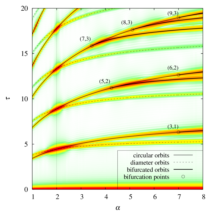
Figure 5: (Color online) Gray-scale plot of the Fourier transform of quantum level density (34) as a function of radial parameter $\alpha$ and scaled period $\tau$. The modulus of the Fourier transform $|F(\tau)|$ has a large value in the dark region. Scaled periods of classical periodic orbits $\tau_{\beta}(\alpha)$ are also shown with lines as functions of $\alpha$. Bifurcation points $(n,m)$ given by Eq. (44) are indicated by open circles.

The scaled periods of classical periodic orbits are also drawn as functions of $\alpha$. One finds an excellent correspondence between Fourier peaks and classical periodic orbits. The peak at $\tau=0$ corresponds to the average level density, which in semiclassical theory is derived from the contribution of the zero-length or direct trajectory. Equally spaced remarkably large peaks for $\alpha=2$ are of a fully degenerate periodic orbit family (and its repetitions) in an isotropic harmonic oscillator [limit of SU(3) symmetry]. If the $\alpha$ is slightly shifted from this value, the orbit family bifurcates into circular orbit and diametric orbit families. With increasing $\alpha$, the circular orbit and its repetitions encounter successive bifurcations at the values given by Eq. (44). One will see that the Fourier peaks associated with the orbits are strongly enhanced around those bifurcation points, indicated by open circles in Fig. 5. This clearly illustrates the significance of periodic-orbit bifurcations to the enhancement of shell effect. One will also note that the maxima of the Fourier amplitudes are slightly shifted towards post-bifurcation side as a general trend. Such shifts have been explained in the semiclassical theory, which is extended to be able to treat bifurcations, e.g., in the improved stationary-phase methodMagner1 ; Magner2 and in the uniform approximationABbridge .

Figure 6: Moduli of Fourier transforms of quantum level density (34) plotted as functions of scaled period $\tau$ for (a) $\alpha=4.0$, (b) 5.0, and (c) 8.0. The peaks associated with the periodic orbits are labeled by their indices $(n,m)$. (2,1) represents a diametric orbit, C represent a circular orbit, and $k(n,m)$ represents the $k$th repetition of the primitive orbit $(n,m)$. In panel (a), the scaled periods of (7,3) and 3C orbits are so closed that the Fourier transform is not resolved into their individual peaks; the same for (5,2) and 2C orbits in panel (b), and for (3,1) and C orbits in panel (c).

III.3 Bifurcation enhancement effect to the shell structures

In order to see the effect of bifurcations of orbits (7,3), (5,2), and (3,1), we examine the shell structures at $\alpha=4.0$, 5.0, and 8.0 where the Fourier amplitudes corresponding to the above orbits are most enhanced. Figure 6 shows the moduli of Fourier amplitudes $|F(\tau)|$ for the above values of radial parameter $\alpha$ (the cross sectional view in Fig. 5 along the vertical lines at those values of $\alpha$). Figure 7 shows the oscillating part of the coarse-grained level densities with two choices of smoothing parameter, $\varGamma=0.24$ for extracting only the gross shell structures and $\varGamma=0.12$ for additional finer structures.

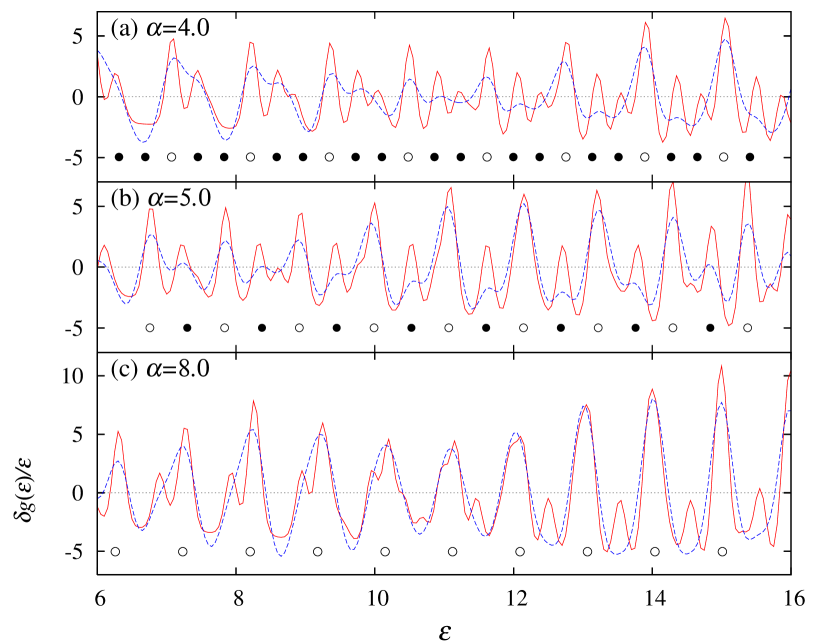
Figure 7: (Color online) Oscillating part of the coarse-grained scaled-energy level density $\delta g(\mathcal{E})$ divided by $\mathcal{E}$ in the spherical power-law potential model with (a) $\alpha=4.0$, (b) 5.0 and (c) 8.0. Solid and dashed lines show results with smoothing width $\varGamma=0.12$ and 0.24, respectively. In panel (a), dots are placed with interval $\delta\mathcal{E}=0.38$, which approximately coincide with the positions of level density maxima. The level density takes relatively larger values at the open dots. The dots in panels (b) and (c) are placed with intervals $\delta\mathcal{E}=0.54$ and 0.97, respectively, which also coincide with the positions of level density maxima. (Physically, the level density minima have more significance, but the supershell structures are clearer for the maxima in these plots.)

In Fig. 6(a), one sees the largest (except for $\tau=0$) peak at $\tau\sim 16.5$, which corresponds to the third repetitions of the circular orbit, 3C ($3\tau_{\rm C}=16.539$), as well as orbit (7,3) ($\tau_{7,3}=16.410$) bifurcated from 3C at $\alpha=31/9=3.44$. These orbits are expected to make dominant contributions in the periodic orbit sum (28), and the pitch of the level density oscillation should be given by $\delta\mathcal{E}=2\pi/\tau_{\beta}\approx 0.38$. The oscillating level density shown in Fig. 7(a) has the period of oscillation just as predicted above. One also note that the oscillation is regularly modulated and the amplitude becomes relatively large for every three oscillations. This is a typical supershell structure caused by the interference of period-3 and period-1 orbits.

Figure 8: Shell energy for (a) $\alpha=4.0$, (b) 5.0, and (c) 8.0, as functions of the cubic root of particle number, taking account of the spin degeneracy factor.

In Fig. 6(b), one sees a prominent peak at $\tau\simeq 11.6$ associated with the second repetitions of the circular orbit, 2C ($2\tau_{\rm C}=11.690$), as well as orbit (5,2) ($\tau_{5,2}=11.609$) bifurcated from 2C at $\alpha=4$. The contribution of these orbit to the level density should be the oscillating function of scaled energy $\mathcal{E}$ with the period $\delta\mathcal{E}\approx 0.54$. The oscillating level density shown in Fig. 7(b) has just the same period as predicted above. One also notes that the supershell structure caused by the interference of period-2 and period-1 orbits is manifested.

In Fig. 6(c), one sees a large peak at $\tau\sim 6.5$ associated with the primitive circular orbit C ($\tau_{\rm C}=6.499$) and the orbit (3,1) ($\tau_{3,1}=6.479$) bifurcated from C at $\alpha=7$. The contributions of these orbits bring about the oscillation of the level density with period $\delta\mathcal{E}\approx 0.97$. The calculated quantum level density in Fig. 7(c) shows the behavior just as expected.

The above shell and supershell structures are also reflected in the shell energy shown in Fig. 8. In panels (a) and (b), the subshell structures due to period-3 and period-2 orbits, respectively, can be found for large $N$ ($N^{1/3}\gtrsim 6$), although they are not so evident in comparison with those found in the level density due to the reduction factor $T_{\beta}^{-2}$ in the trace formula of shell energy (3). In panel (c) of Fig. 8, one sees a remarkable enhancement of major shell effects compared with the other panels. This is regarded as the result of bifurcation enhancement effect of the circular orbit. Note that the plots in Figs. 7 and 8 are extended to large $\mathcal{E}$ and $N$ (far beyond the region of existing nuclei, but this may be meaningful for metallic clusters), where the above shell and supershell structures become more evident. Unfortunately, the subshell structures for $\alpha=4.0$ and 5.0 in shell energies are not very prominent in the existing nuclear region and they might disappear, e.g., after including the spin-orbit coupling, but the pronounced shell effect for $\alpha\sim 8.0$ might survive and be responsible for enhancement of shell effects in real nuclei around the medium-mass to heavy region.

IV Spheroidal deformations

IV.1 Shape parametrization and quantum spectra

Figure 9: Poincaré surface of section $\{(x,p_{x})|z=0\}$ for meridian-plane orbits in spheroidal-shape potentials with axis ratio $\eta=\sqrt{3}$ ($\delta\approx 0.49$) and with several values of radial parameter $\alpha$. The origin $(x=p_{x}=0)$ corresponds to the orbit Z, and the outer boundary corresponds to the orbit X.

An axially symmetric anisotropic harmonic oscillator potential system is integrable, and it has a spheroidal equipotential surface. It is known that a spheroidal deformed cavity (infinite well potential) system is also integrable. For spheroidal deformation, the shape function is expressed as

$$f(\theta)=\left[\frac{\sin^{2}\theta}{(R_{\perp}/R_{0})^{2}}+\frac{\cos^{2}\theta}{(R_{z}/R_{0})^{2}}\right]^{-1/2}$$ (51)

where $R_{z}$ and $R_{\perp}$ represent lengths of semiaxes of the spheroid which are parallel and perpendicular to the symmetry axis ($z$ axis), respectively, and $R_{0}$ is their spherical value. Taking account of the volume conservation condition $R_{\perp}^{2}R_{z}=R_{0}^{3}$, we define the deformation parameter $\delta$ as

$$R_{\perp}=R_{0}e^{-\delta/3},\quad R_{z}=R_{0}e^{2\delta/3}.$$ (52)

It is related to the axis ratio $\eta=R_{z}/R_{\perp}$ by $\eta=e^{\delta}$. The spherical shape $\eta=1$ corresponds to $\delta=0$ and prolate/oblate superdeformed shapes $\eta=2^{\pm 1}$ correspond to $\delta=\pm\ln 2\approx\pm 0.69$. The system with spheroidal power-law potential is nonintegrable except for two limits, $\alpha=2$ (HO) and $\alpha=\infty$ (cavity). In Fig. 9, we show the Poincaré surface of section for $\alpha=2,5,20$, and $\infty$, each with $\eta=\sqrt{3}$ ($\delta\approx 0.49$). It is found that some complex structures emerge in the Poincaré plots with increasing $\alpha>2$, and the surface becomes most chaotic around $\alpha\sim 20$, then it turns into simpler structure for extremely large $\alpha$.

Figure 10: Single-particle level diagram for Hamiltonian (11) with spheroidal deformation (51). Scaled-energy levels are plotted as functions of deformation parameter $\delta$ defined by Eq. (52). Solid and broken lines represents levels with even and odd parities, respectively.

Figure 10 shows the single-particle spectra as functions of spheroidal deformation parameter $\delta$. The value of radial parameter is put at $\alpha=5.0$, corresponding to medium-mass nuclei. The degeneracies of levels at the spherical shape are resolved and shell structure changes with varying deformation. The level diagram is similar to what is obtained for MO or WS/BP models without spin-orbit coupling. One of its characteristic features in comparison with the HO model is the asymmetry of deformed shell structures in prolate and oblate sides. This asymmetry becomes more pronounced for larger $\alpha$, and it might be regarded as the origin of prolate-shape dominance in nuclear ground-state deformations. We shall discuss the semiclassical origin of the above asymmetry in the following subsections.

Figure 11: Same as Fig. 9 but for quadrupole deformations $\beta_{2}=0.3$ and $0.4$ with $\alpha=5.0$.

In order to see the dependence on shape parametrization, we also calculated the deformed quantum spectra for quadrupole deformation, which might be more popular in earlier studies:

$$f(\theta)=\frac{1+\beta_{2}P_{2}(\cos\theta)}{\sqrt[3]{1+\frac{3}{5}\beta_{2}^{2}+\frac{2}{35}\beta_{2}^{3}}}.$$ (53)

The factor in the denominator arranges the conservation of volume surrounded by equipotential surface. Figure 11 show Poincaré surface of section for quadrupole deformations $\beta_{2}=0.3$ and $0.4$ with $\alpha=5.0$. Comparing with the Fig. 9(b), one will see that the particle motions in the quadrupole potential are more chaotic than those in the spheroidal potential.

Figure 12: Same as Fig. 10 but as functions of quadrupole deformation parameter $\beta_{2}$.

Figure 12 shows the level diagram for quadrupole deformation. Although the properties of classical motion are quite different from those in spheroidal potential, the deformed shell structures are very similar to each other. Thus, the above difference of shape parametrization does not cause a serious difference in the gross shell structures at normal deformations. Notable effects of chaoticity in the quadrupole potential can only be seen in the strong level repulsions at large deformations $\beta_{2}\gtrsim 0.3$. Therefore, we shall only consider the spheroidal deformation in the following analysis.

IV.2 Prolate-oblate asymmetry in deformed shell structures

Let us examine the properties of deformed shell structures in the normal deformation region ($|\delta|\lesssim 0.3$). As shown in Figs. 10 and 12, single-particle spectra in a potential with a sharp surface show prolate-oblate asymmetry (in the sense discussed in Sec. I). Hamamoto and MottelsonHamMot paid attention to the different ways of level fanning (from the terminology used in Ref. HamMot ) in oblate and prolate sides; level fanning is considerably suppressed in the oblate side as compared to the prolate side. Due to that suppression of level fanning, shell structures in the oblate shapes are similar to those of the spherical shape, and the system has a smaller chance to gain shell energy by means of oblate deformation. This may explain the feature of prolate-shape dominance. They have shown that the above asymmetric way of level fanning can be understood from the interaction between single-particle levels, which acts to suppress the level repulsions in the oblate side for a potential with sharp surface. It clearly explains the fact that the asymmetry becomes more pronounced for heavier nuclei, e.g., in the Woods-Saxon modelStrMag . The same kind of asymmetry is also found in the spectrum of the Nilsson model.

In the spheroidal power-law potential model, the asymmetry in level fanning becomes more pronounced for larger $\alpha$ as expected. In Fig. 13(b), fannings of some $nl$ levels ($n$ and $l$ represent principal and azimuthal quantum numbers, respectively) are illustrated for $\alpha=5.0$. One sees that the level fannings are considerably suppressed in the oblate side as in the cavity potential.

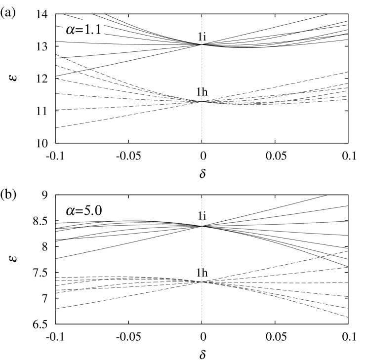
Figure 13: Fanning of single-particle levels 1h (dashed lines) and 1i (solid lines) for (a) $\alpha=1.1$ and (b) 5.0.

It is interesting to note that, if we take the radial parameter $\alpha<2$ (although it does not correspond to actual nuclear situations), the way of level fanning becomes just opposite to the case of $\alpha>2$. As one sees in Fig. 13(a), level spreading is suppressed in the prolate side. We will discuss later if it causes oblate-shape dominance.

Following the analysis in Ref. HamMot , we calculate the deformation energy

$$E_{\rm def}(A,\delta)=E(A,\delta)-E(A,0)$$ (54)

and compare the energies in prolate and oblate sides at each local minima. Here, we assume the same single-particle spectra for neutrons and protons and only consider $N=Z$ even-even nuclei for simplicity. The sum of single-particle energies for nucleus of mass number $A$ is given by

$$E_{\rm sp}(A)=4\sum_{i=1}^{n}e_{i},\quad A=N+Z=4n.$$ (55)

Using the Strutinsky method, the above energy can be decomposed into a smooth part $\tilde{E}_{\rm sp}(A)$ and an oscillating part $\delta E(A)$. As in usual, we can expect that the above oscillating part represents the correct quantum shell effect of a many-body system. In Strutinsky’s shell correction method, the smooth part is replaced with the phenomenological liquid drop model (LDM) energy to get the total many-body energy, but here we try to extract the smooth part also from the single-particle energies. In mean-field approximation, the single particle Hamiltonian is written as

$$\hat{h}=\hat{t}+\hat{u},$$ (56)

where $\hat{t}$ and $\hat{u}$ represent kinetic energy and mean-field potential, respectively, and $\hat{u}$ is currently given by the power-law potential. In this case, by the use of the Virial theorem, the average of $\hat{t}$ and $\hat{u}$ are in the ratio $2\langle\hat{t}\rangle=\alpha\langle\hat{u}\rangle$, and one obtains

$$\langle\hat{t}\rangle=\frac{\alpha}{\alpha+2}\langle\hat{h}\rangle,\quad\langle\hat{u}\rangle=\frac{2}{\alpha+2}\langle\hat{h}\rangle.$$ (57)

Therefore, the smooth (average) part of the $A$-body energy is given approximately by

$$\tilde{E}(A)\approx\left\langle\sum_{i}\hat{t}_{i}+\frac{1}{2}\sum_{i}\hat{u}_{i}\right\rangle=\frac{\alpha+1}{\alpha+2}\,\tilde{E}_{\rm sp}(A)$$ (58)

This expression will be valid for many-body systems interacting with two-body interaction. Thus, we evaluate the $A$-body energy by

$$E(A)=\frac{\alpha+1}{\alpha+2}\tilde{E}_{\rm sp}(A)+\delta E(A)$$ (59)

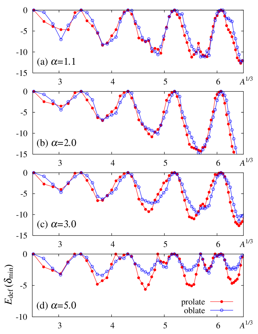
Figure 14: (Color online) Deformation energies (54) of prolate and oblate states at each local minima. Deformation energy $E_{A}(\delta)$ is calculated as a function of deformation $\delta$ and its minimum values for prolate and oblate sides are plotted with filled and open circles, respectively.

Figure 14 compares the local minima of deformation energies (54) in prolate and oblate sides. At the HO value [$\alpha=2.0$, panel (b)], prolate and oblate deformed shell structures are symmetric and the deformation energies are comparable with each other. For $\alpha>2$ [panels (c) and (d) of Fig. 14], the deformation energies in the prolate side become considerably lower than in the oblate side as the radial parameter $\alpha$ becomes larger. The power-law potential model thus reproduce correctly the feature of prolate-shape dominance in nuclear deformation.

For $\alpha<2$, as shown in Fig. 14(a), we find no indication of oblate-shape dominance in spite of the feature of level fanning shown in Fig. 13(a). One finds some lowest energy states at oblate shapes $\delta\sim-0.3$, but the difference in energies between prolate and oblate minima are generally small. Therefore, one cannot fully explain the prolate(oblate)-shape dominance only by the ways of level fanning.

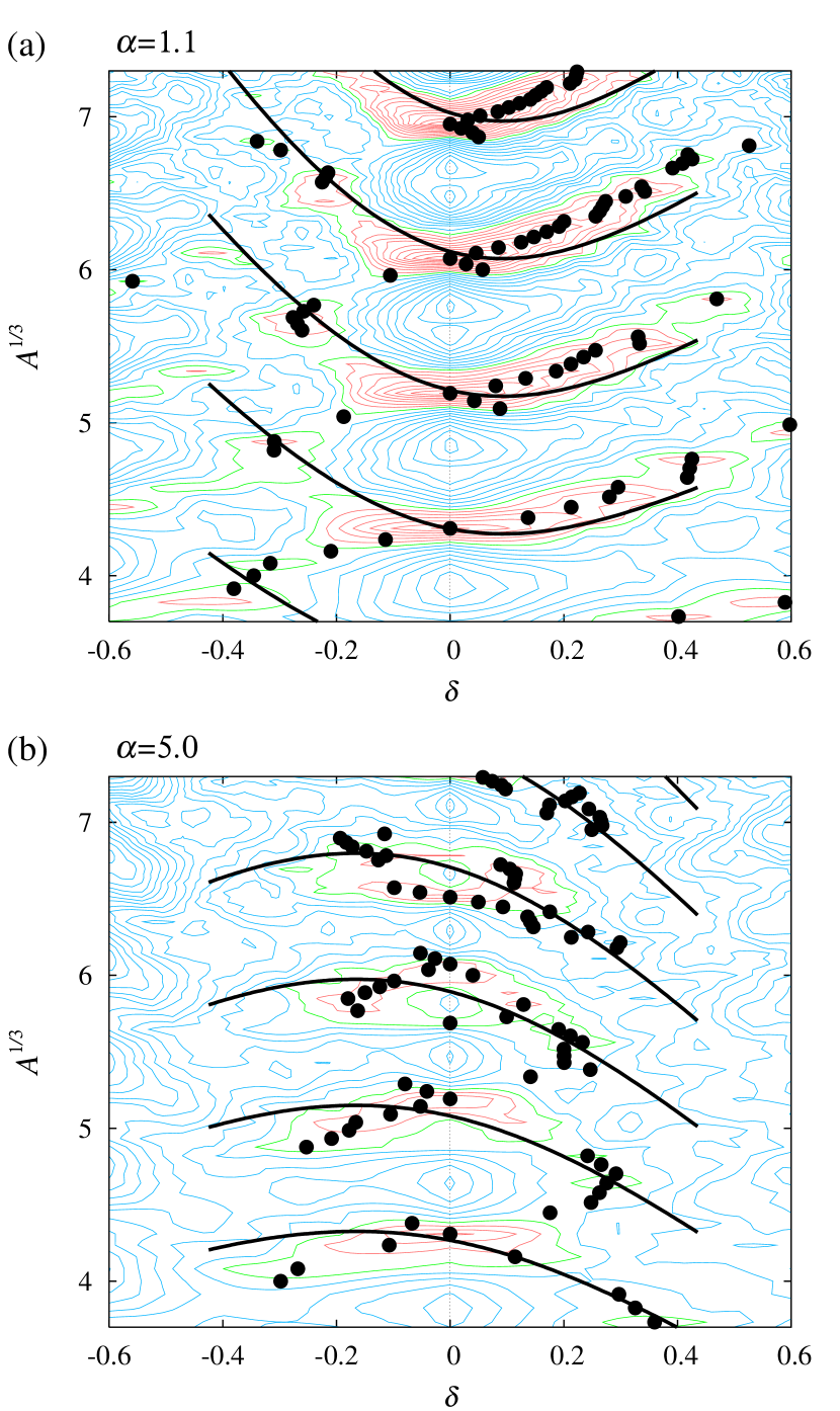
Figure 15: (Color online) Contour plot of the $A$-body shell-deformation energy (60) in the deformation-mass number plane $(\delta,A^{1/3})$ for (a) $\alpha=1.1$ and (b) 5.0. Solid and dashed contour lines represent negative and positive values, respectively. Dots represent values of the deformation parameter at absolute energy minima for each $A$. Thick solid curves represent constant-action lines (66) for bridge orbit M(1,1).

In order to analyze shape stability, we define shell-deformation energy using the smooth part of the energy at spherical shape as a reference,

$$\Delta E(A,\delta)=E(A,\delta)-\tilde{E}(A,0),$$ (60)

with Eqs. (58) and (59). [Note that the second term on the right-hand side of Eq. (60) is not $\tilde{E}(A,\delta)$, so that $\Delta E$ contains the smooth part of the deformation energy.] Figure 15 shows contour plots of $\Delta E$ for $\alpha=1.1$ and $5.0$ as functions of deformation $\delta$ and mass number $A$. They show some deep minima along the $\delta=0$ axis at values of $A$ corresponding to spherical magic numbers. The energy valleys run through these minima and the deformation energy minima distribute along them. For $\alpha=5.0$, the valley lines in the $(\delta,\tau)$ plane have large slopes in the prolate side and deep energy minima are formed around $\delta\sim 0.2$ for mass numbers at the middle of adjacent spherical magic numbers, while the valley lines are almost flat in the oblate side. This is essentially the same behavior as what Frisk found for the spheroidal cavityFrisk . For $\alpha=1.1$, the valley lines have larger slope in the oblate side, but the slope in the prolate side is not as small as in the oblate side for $\alpha=5.0$ and the deformation energy minima distribute mainly along the valley lines in the prolate side. One can find rather deep energy minima at $\delta\sim-0.3$ for particle numbers between the spherical magic numbers, but the energy difference between oblate and prolate local minima are generally small. Thus, for an understanding of prolate-shape dominance, it is critical to explain the asymmetric behavior of the slopes of the energy valleys.

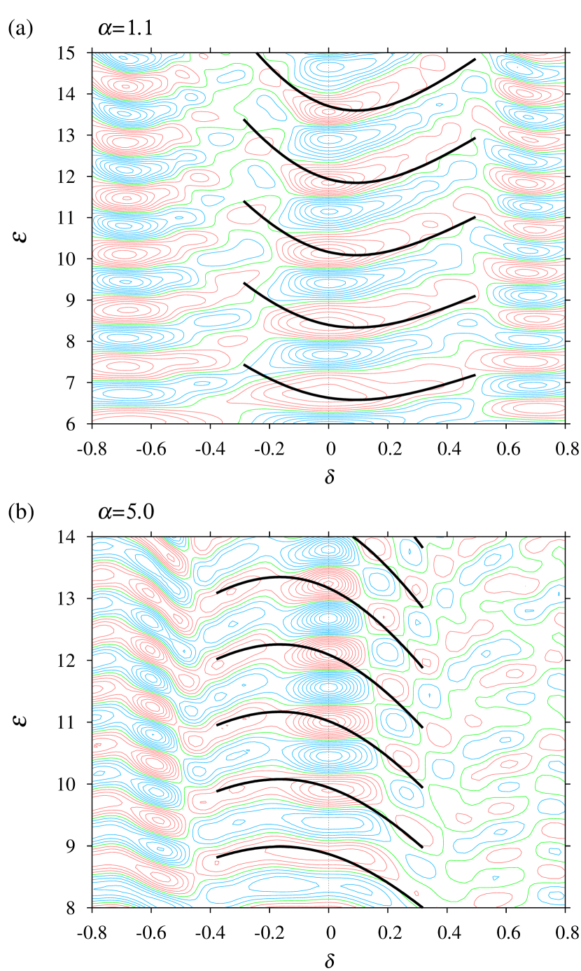
Figure 16: (Color online) Contour plot of oscillating level density for radial parameter (a) $\alpha=1.1$ and (b) 5.0 in deformation-energy plane $(\delta,\mathcal{E})$. For calculation of coarse-grained level density, smoothing width $\Delta\mathcal{E}=3.0$ is taken. Solid and dashed contour lines represent negative and positive values, respectively. Thick solid lines represent constant-action lines (63) for the bridge orbits M(1,1).

Since shell energy takes a deep negative value when the single-particle level density at the Fermi energy is low, let us investigate the coarse-grained single-particle level density as functions of energy and deformation. Figure 16 shows the oscillating part of course-grained single-particle level density for $\alpha=1.1$ and $5.0$ plotted as functions of deformation $\delta$ and scaled energy $\mathcal{E}$. They show regular ridge-valley structures similar to the shell energy. Therefore, for an understanding of prolate-shape dominance, it is essential to investigate the origin of the above ridge-valley structures in the deformed single-particle level density. For the spheroidal cavity potential, Frisk ascribed it to the change of the action integrals along the triangular and rhomboidal orbits in the meridian plane, for which the volume conservation condition plays an important roleFrisk . We are going to study the case of the more realistic power-law potential.

In the following subsections, we will show that the above ridge-valley structure can be explained in connection with classical periodic orbits using semiclassical periodic-orbit theory. The thick solid curves in Figs. 15 and 16 represent the semiclassical prediction of the valley lines which will be discussed in Sec. IV.4.

IV.3 Periodic orbits in spheroidal potential

In order to examine the semiclassical origin of the above asymmetry in a deformed shell structure using periodic orbit theory, we first consider the properties of classical periodic orbits in the spheroidal power-law potential and their bifurcations. For the spherical potential, all the periodic orbits are planar and degenerate with respect to rotations. The degree of degeneracy for the orbit family is described by degeneracy parameter $\mathcal{K}$ which represents the number of independent continuous parameters required to specify a certain orbit in the family. The maximum value of $\mathcal{K}$ is equal to the number of independent symmetric transformations of the system. The isolated orbits have $\mathcal{K}=0$. In the spherical cavity potential, degeneracy parameter is $\mathcal{K}=3$ for generic periodic orbits, and $\mathcal{K}=2$ for diametric and circular orbits which are transformed onto themselves by one of the rotations. If the spheroidal deformation is added to the potential, generic planar orbits bifurcate into two branches: One is the orbit in the equatorial plane and the other is the orbit in the meridian plane (the plane containing the symmetry axis). All but two exceptional orbits degenerate with respect to the rotation about the symmetry axis, and the degeneracy parameter is $\mathcal{K}=1$. The diametric orbit bifurcate into degenerate family of equatorial diametric orbits ($\mathcal{K}=1$) and an isolated diametric orbit along the symmetry axis ($\mathcal{K}=0$). The circular orbit bifurcates into an isolated equatorial circular orbit ($\mathcal{K}=0$) and an oval-shape orbit in the meridian plane ($\mathcal{K}=1$). With increasing deformation towards prolate side $(\delta>0)$, the equatorial orbits undergo successive period $m$-upling bifurcations and new 3D orbits emerge. In the oblate side, the diametric orbit along the symmetry axis undergoes successive period $m$-upling bifurcations and generates new meridian-plane orbits. These new-born 3D and meridian-plane orbits have hyperbolic caustics and are sometimes called hyperbolic orbits.

It is very interesting to note that the above new-born hyperbolic orbits from equatorial orbits are distorted towards the symmetry axis with increasing deformation and finally submerge into the diametric orbit along the symmetry axis. (Some 3D orbits submerge into other hyperbolic orbits before submerging into the symmetry-axis orbit at last.) In this way, the hyperbolic orbits make bridges between the equatorial and symmetry-axis orbits, and we shall call those hyperbolic orbits “bridge orbits”ABbridge ; BarDav87 . With increasing $\delta$, periods of the equatorial orbit decrease while that of the symmetry-axis orbit increases. At each crossing point of the periods (or actions) of repeated equatorial and symmetry-axis orbits, bridge orbits exist to intervene between them.

Accordingly, we shall classify periodic orbits in the spheroidal power-law potential into the following four groups:

1. Isolated orbits ($\mathcal{K}=0$): This group consists of the diametric orbit along the symmetry axis ($z$-axis), denoted Z, and the circular orbit in the equatorial plane, denoted EC. Orbit EC is stable both in the prolate and oblate sides, whose repeated period $m$-upling bifurcations generate 3D bridge orbits. Orbit Z is stable in the oblate side and undergoes successive period $m$-upling bifurcations, while its stability alternates in the prolate side with repeated bifurcations which absorb bridge orbits.

2. Equatorial-plane orbits ($\mathcal{K}=1$): This corresponds to the equatorial-plane branch of the deformation-induced bifurcation. They have the same shapes as those in the spherical potential shown in Fig. 4. They are denoted E$(k,m)$, where $k$ is the number of vertices (corners) and $m$ is the number of rotation. The diametric orbit is specially denoted X (which includes the orbits along the $x$ axis).

3. Meridian-plane orbits ($\mathcal{K}=1$): This corresponds to the meridian-plane branch of the deformation-induced bifurcation. They survive up to any large deformation, keeping their original geometries.

4. Bridge orbits ($\mathcal{K}=1$): These orbits emerge from the bifurcations of equatorial orbits. Meridian-plane orbits emerge from diametric orbits and submerge into repetitions of orbit Z. Nonplanar 3D orbits emerge from nondiametric equatorial orbits, and they also submerge into the orbit Z. Some of them submerge into other bridge orbits before submerging into Z. The meridian-plane bridge which rests between $m$X ($m$th repetition of X) and $n$Z ($n$th repetition of Z) is denoted M$(m,n)$. Except for the M(1,1) bridge, a pair of stable and unstable bridge orbits emerge, and are denoted M$(m,n)_{s}$ and M$(m,n)_{u}$, respectively. 3D bridge B$(m,m,n)$ emerges via pitchfork bifurcation of equatorial $m$EC ($m$th repetitions of EC), and submerges into M$(m,n)$ orbit before finally submerging into $n$Z. The other 3D bridges intervening between equatorial E$(k,m)$ and $n$Z emerge as a stable and unstable pair, and are denoted as B$(k,m,n)_{s,u}$. With increasing deformation, they first submerge into 3D bridge B$(m,m,n)$, which will submerge into M$(m,n)$ and finally into $n$Z.

Figure 17: Bifurcation diagram for the M(1,1) bridge orbit between the X and Z orbits for $\alpha=3.0$. Traces of the symmetry-reduced monodromy matrix $\tilde{\mathbf{M}}$ are plotted as functions of deformation parameter $\delta$. Bifurcation points ($\mathop{\rm Tr}\tilde{\mathbf{M}}=2$) are indicated by open circles. Shapes of the periodic orbits as well as the equipotential surface are also shown.

Figure 17 shows the bifurcation diagram for bridge orbit M(1,1) for $\alpha=3.0$. The traces of $(2\times 2)$ symmetry-reduced monodromy matrices for relevant periodic orbits are plotted as functions of deformation parameter $\delta$. The $\mathcal{K}=1$ family of equatorial diameter orbits X undergoes pitchfork bifurcation at $\delta=-0.34$ and a family of oval-shape meridian-plane orbits M(1,1) emerge. In the limit $\delta\to 0$, the shape of the M(1,1) orbit approaches a circle, and it associates with equatorial circular orbit EC to form a $\mathcal{K}=2$ family. At $\delta>0$ it bifurcates into an equatorial EC and a meridian M(1,1) family again. The meridian branch submerges into the orbit Z at $\delta=0.34$ via pitchfork bifurcation. Thus, the orbits M(1,1) make a bridge between two diametric orbits X and Z.

In the HO limit, $\alpha\to 2$, the bridge shrinks to a crossing point of X and Z orbits and can exist only at $\delta=0$ (spherical shape), where they altogether form a degenerate $\mathcal{K}=2$ family. With increasing $\alpha$, the bridge orbit exists in a wider range of deformation over the crossing point. In the cavity limit, $\alpha\to\infty$, this orbit approaches the so-called creeping orbit or whispering gallery orbit, which runs along the boundary.

IV.4 Semiclassical origin of prolate-oblate asymmetry

To see the effect of the above bifurcation on the shell structure, we calculate Fourier transform of level density (34) with the obtained quantum spectra. In Fig. 18, modulus of Fourier transform $|F(\tau,\delta)|$ is shown in a gray-scale plot as a function of deformation $\delta$ and scaled period $\tau$. Scaled periods of classical periodic orbits $\tau_{\beta}(\delta)$ are also drawn by lines. One sees a nice correspondence between the quantum Fourier amplitude and classical periodic orbits. Particularly, one can find significant peaks along the bridge orbit M(1,1), which indicate that the shell structure in the normal deformation region is mainly determined by the contribution of this bridge orbit.

Let us assume that a contribution of single orbit (or degenerate family) $\beta$ dominates the periodic orbit sum, namely,

$$\delta g(\mathcal{E})\approx A_{\beta}\cos(\mathcal{E}\tau_{\beta}-\tfrac{\pi}{2}\nu_{\beta}).$$ (61)

Then, the valley lines of level density should run along the curves where the above cosine function takes the minimum value $-1$, namely,

$$\mathcal{E}\tau_{\beta}-\frac{\pi}{2}\nu_{\beta}=(2n+1)\pi,\quad n=0,1,2,\cdots.$$ (62)

In Fig. 16, we plot these constant-action lines

$$\mathcal{E}=\frac{(2n+1+\frac{1}{2}\nu_{\beta})\pi}{\tau_{\beta}(\delta)}$$ (63)

for bridge orbit M(1,1). We see that the constant-action lines of the bridge orbit nicely explain the ridge-valley structure in the quantum level density. The slight disagreement of constant-action lines and the bottom of the energy valleys might be due to interference between other PO contributions.

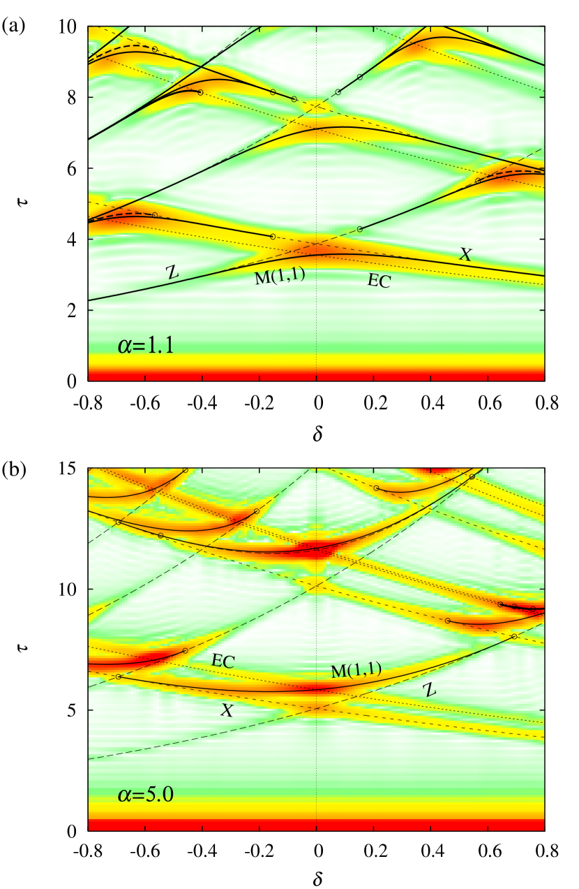
Figure 18: (Color online) Modulus of the Fourier transform of the level density is shown by gray-scale plot as a function of deformation parameter $\delta$ and scaled period $\tau$. Scaled periods of classical periodic orbits are also displayed.

The shell energy is also given by the periodic-orbit contribution as

$$\delta\mathcal{E}(N)\approx\frac{A_{\beta}}{\tau_{\beta}^{2}}\cos[\mathcal{E}_{F}(N)\tau_{\beta}-\tfrac{\pi}{2}\nu_{\beta}],$$ (64)

where $\mathcal{E}_{F}$ represents Fermi level, which is approximately given by

$$\mathcal{E}_{F}(N)\approx\left[3N/c_{0}(\alpha)\right]^{1/3}$$ (65)

which is derived from the leading term of Eq. (25). Thus, the shell energy takes large negative values along the constant-action lines for dominant orbit $\beta$:

$$\mathcal{E}_{F}\approx\left(\frac{3}{c_{0}(\alpha)}\,\frac{A}{4}\right)^{1/3}=\frac{(2n+1+\tfrac{1}{2}\nu_{\beta})\pi}{\tau_{\beta}(\delta)}.$$ (66)

In Fig. 15, we also plot the above constant-action lines for bridge orbits M(1,1) with thick solid lines. They satisfactorily explain the valley lines of shell energy. Distribution of deformed shell energy minima in Fig. 15 are thus understood as the effect of bridge orbit contribution.

For $\alpha>2$, bridge orbits appear upward from the crossing point of two diametric orbits X and Z in the $(\delta,\tau)$ plane. Note that the scaled action of orbit Z has a larger slope than that of orbit X in the $(\delta,\tau)$ plane. This difference comes from the fact that the lengths of semiaxes $R_{z}$ and $R_{\perp}$ in a volume-conserved spheroidal body are proportional to the different powers of deformation parameter $\delta$ as in Eq. (52). The scaled period of the diametric orbit along the $i$th axis is proportional to the length of corresponding semiaxis $R_{i}$,

$$\tau_{i}=\tau_{0}^{D}\frac{R_{i}}{R_{0}},$$

where $\tau_{0}^{D}$ is the scaled period of the diametric orbit at spherical shape. Using Eq. (52), one has

$$\tau_{X}=\tau_{0}^{D}e^{-\frac{1}{3}\delta},\quad\tau_{Z}=\tau_{0}^{D}e^{\frac{2}{3}\delta}.$$ (67)

Therefore, the bridge between X and Z orbits has a large slope in the prolate side while it is almost flat in the oblate side. This clearly explains the profile of ridge-valley structures in level density and shell energy. With increasing $\alpha$, triangular- and square-type orbits emerge at $\alpha=7$ and $14$, respectively, via the isochronous bifurcations of the circular orbit [see Eq. (44) for $m=1$] for spherical shape. With spheroidal deformation, they bifurcate into equatorial and meridian branches, which are both singly degenerated due to the axial symmetry. For finite $\alpha$, they submerge into oval orbits and finally into diametric orbits at large deformations. In this sense, they are also bridge orbits intervening between two diametric orbits. These meridian orbits survive up to larger deformation with increasing $\alpha$, and in the cavity limit ($\alpha\to\infty$), they survive for any large deformation. Therefore, the meridian orbits in the cavity potential can be regarded as a limit of bridge orbits. Thus we see that Frisk’s argument for a spheroidal cavity systemFrisk is continuously extended to the case of finite diffuseness.

For $\alpha<2$, a bridge orbit appear in the opposite side of the crossing point and its slope becomes larger in the oblate side. This also explains the profile of valley lines in level density and shell energy for $\alpha=1.1$ as shown in Figs. 16(a) and 15(a).

IV.5 Superdeformed shell structures

In the axially deformed harmonic oscillator (HO) potential model, one sees simultaneous degeneracy of many energy levels at rational axis ratios. The HO model is often used for the nuclear mean-field potential in the limit of light nuclei. In the HO model, superdeformation is explained as the result of strong level bunching at axis ratio 2:1. A search for much larger deformation originated from the strong level bunching at axis ratio 3:1 (sometimes referred to as hyperdeformation) has also been a challenging experimental and theoretical problem. On the other hand, the spheroidal cavity model, which is used as the limit of potential for heavy nuclei, also shows superdeformed shell structures, while the shell effect is much weaker than that found in the oscillator model. In the spheroidal cavity model, superdeformed shell structures are intimately related with emergence of meridian and 3D orbits which oscillate twice in the short axis direction while they oscillate once in the long-axis direction, just as the degenerate 3D orbits in the 2:1 axially-deformed HO potentialASM . One may expect to have a unified semiclassical understanding of the origin of superdeformed shell structures found in the above two limiting cases by connecting them with the power-law potential model.

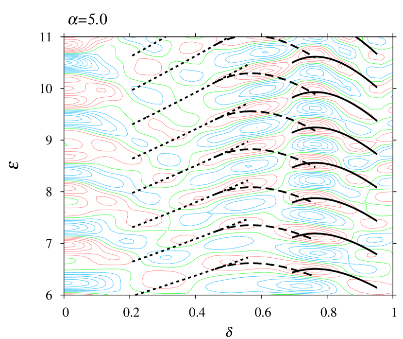
Figure 19: (Color online) Contour plot of oscillating level density for radial parameter $\alpha=5.0$ around a prolate superdeformed region. Smoothing width $\varGamma=0.2$ is used. Solid and dashed contour lines represent negative and positive values, respectively. Thick dotted, dashed and solid lines represent constant action lines (63) of periodic orbits 2X, M(2,1), and B(2,2,1), respectively.

Figure 19 shows the oscillating part of the coarse-grained level density for radial parameter $\alpha=5.0$ and deformation $\delta$ around a superdeformed region. It clearly show that new regularities in shell structure are formed at a superdeformed region. The valley lines are up-going till $\delta\sim 0.5$, and they bend down around $\delta\sim 0.6$. One sees another deep minima at $\delta\gtrsim 0.7$. Let us examine their semiclassical origins.

For $\alpha>2$, one finds bridge orbits M(2,1) which intervenes between orbits 2X (second repetitions of X) and Z. Figure 21 is the bifurcation diagram for the orbits relevant to this bifurcation, calculated for $\alpha=3.0$. The orbit X undergoes a period-doubling bifurcation at $\delta=0.55$ and there emerges a pair of bridge orbits M$(2,1)_{s}$ (stable) and M$(2,1)_{u}$ (unstable). They have shapes of a boomerang and a butterfly as shown in Fig. 21. With increasing $\delta$, those orbits are distorted toward the $z$ axis and finally submerge into the orbit Z at different values of $\delta$ via pitchfork bifurcations.

Figure 20: Same as Fig. 17 but for the M(2,1) bridge orbit between 2X and Z; “2X” represents the second repetition of X. The radial parameter $\alpha=3.0$ is used. A pair of bridge orbits emerge at $\delta=0.55$ via period-doubling bifurcation. The unstable branch M$(2,1)_{u}$ and stable branch M$(2,1)_{s}$ submerge into Z at $\delta=0.80$ and 0.97, respectively, via pitchfork bifurcations.

Figure 21: 3D orbits responsible for the superdeformed shell structure at $\delta\sim 0.7$ and $\alpha=5$. 3D plots and projections on $(x,y)$, $(x,z)$, and $(y,z)$ planes are shown as well as equipotential surfaces. B$(5,2,1)_{s}$ and B$(5,2,1)_{u}$ are a pair of stable and unstable 3D orbits that emerged from equatorial orbit E(5,2). B(2,2,1) emerged from the second repetition of the equatorial circular orbit, 2EC.

For larger $\alpha$, various equatorial orbits appear as shown in Fig. 4, and they also undergo bifurcations by imposing deformation. Each of those bifurcations will generate a pair of 3D bridge orbits, which are also distorted toward the symmetry axis by increasing $\delta$ and finally submerge into Z. Figure 21 shows some 3D bridge orbits important for superdeformed shell structures for $\alpha=5.0$. Equatorial circular orbit EC undergoes a period-doubling bifurcation, which is peculiar to 3D systems, and generates 3D bridge orbit B(2,2,1). Equatorial orbit E(5,2) undergoes a nongeneric period-doubling bifurcation and a pair of 3D bridge orbits B$(5,2,1)_{s,u}$ emerge. All the above 3D orbits finally submerge into the Z orbit by increasing deformation $\delta$. See the Appendix for a detailed description of these 3D bridge orbit bifurcations.

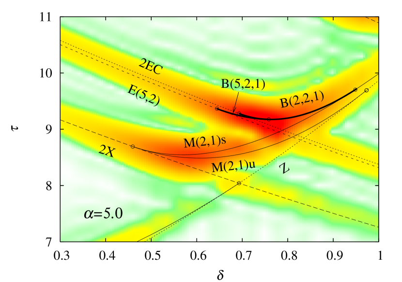
Figure 22: (Color online) Gray-scale plot of the Fourier transform of the quantum level density (34) for radial parameter $\alpha=5.0$ as a function of deformation $\delta$ and scaled period $\tau$. The modulus of the Fourier transform has a large value in the dark region. The scaled periods of classical periodic orbits $\tau_{\beta}$ are displayed with lines. Their bifurcation points are indicated by open circles.

Figure 22 shows the Fourier transform of scaled-energy level density for $\alpha=5.0$ around a superdeformed region. The scaled periods of classical periodic orbits are also drawn with lines. The Fourier amplitude shows remarkable enhancement along the bridge orbits M(2,1) and B(5,2,1), indicating their significant roles in superdeformed shell structures.

The constant action lines (63) for M(2,1) and B(2,2,1) are shown in Fig. 19 with thick solid and broken lines. They perfectly explain the ridge-valley structures of quantum level densities. This shows the significant roles of bifurcations of M(2,1) and B$(n,2,1)$ orbits for enhanced shell effects at $\delta\sim 0.5$ and 0.7, respectively.

M(2,1) and B(2,2,1) orbits shrink to the crossing point of 2X (2EC) and Z orbits in the HO limit, $\alpha\to 2$, and turn into a $\mathcal{K}=4$ degenerate family. With increasing $\alpha$, the deformation range in which a bridge orbit can exist becomes wider. Therefore, the bifurcation deformation of the orbits 2X and 2EC becomes smaller with increasing $\alpha$, and the effect of these orbits takes place at smaller deformation. This may explain the experimental fact that deformations of the superdeformed states are smaller for heavier nuclei; e.g., $\beta_{2}\sim 0.6$ for the Dy region and $\beta_{2}=0.4\mbox{--}0.5$ for the Hg regionTwin ; AAberg . In the cavity limit $\alpha\to\infty$, the two meridian orbits M(2,1) and the two 3D orbits B($n$,2,1) respectively join to form $\mathcal{K}=1$ families, which survive for arbitrary large deformations.Hide ; ASM

In conclusion, the highly degenerate family of orbits in the rational HO potential ($\alpha=2$) are resolved at $\alpha>2$ into two orbits: equatorial and symmetry-axis orbits that have fewer degeneracies, and the bridge orbit which mediates between them within a finite deformation range. The “length” of the bridge in the $(\delta,\tau)$ plane grows with radial parameter $\alpha$, and the superdeformed shell structures are formed in smaller $\delta$ for large $\alpha$, corresponding to heavier nuclei, due to the strong shell effect brought about by the bridge-orbit bifurcation. In the $\alpha\to\infty$ limit, some of the simplest bridge orbits coincide with meridian and 3D orbits emerging from the bifurcation of equatorial orbits at $\delta=0.5\mbox{--}0.6$ which play a significant role in superdeformed shell structures in the spheroidal cavity modelASM ; Magner2 . Thus, the semiclassical origins of superdeformed and hyperdeformed shell structures in the HO and the cavity models are unified as the two limiting cases of the contribution of bridge-orbit bifurcations in power-law potential model.

V Summary

We have made a semiclassical analysis of deformed shell structures with the radial power-law potential model, which we introduce as a realistic nuclear mean-field model (except for the lack of a spin-orbit term in the current version) for stable nuclei in place of WS/BP models. We have shown that bridge orbits mediating equatorial and symmetry-axis orbits play a significant role in normal and superdeformed shell structures. Particularly, prolate-oblate asymmetry of deformed shell structures, which is responsible for the prolate dominance in nuclear deformations, is clearly understood as the asymmetric slopes of bridge orbits in the $(\delta,\tau)$ plane. This asymmetry grows with increasing radial parameter $\alpha$, and thus with increasing mass number $A$, which explains the fact that the prolate dominance is more remarkable in heavier nuclei. Some of these bridge orbits coincide with triangular and rhomboidal orbits in the cavity limit $\alpha=\infty$, whose significant contribution to the coarse-grained level density in a spheroidal cavity and their roles in prolate-shape dominance were discussed by Frisk. Our results elucidate that the essence of the semiclassical origin of prolate-shape dominance in the cavity model also applies to the more realistic power-law potential model. The semiclassical origin of superdeformed shell structures which have been discussed separately for oscillator and cavity models are continuously connected via bridge orbits in power-law potential models.

In this paper we have explored the contribution of periodic orbits via Fourier transform of the quantum level density. In order to clarify the role of periodic-orbit bifurcation to the level density, it is important to establish a semiclassical method with which we can evaluate contribution of classical periodic orbits in the bifurcation region. Some preliminary results for the spherical power-law potential using the improved stationary phase method have been reported in Ref. MAB2011 . Application of a uniform approximation to this problem is also in progress.

Another important subject is the inclusion of spin degrees of freedom. Since the nuclear mean field has strong spin-orbit coupling, it should be crucial to take account of its effect to analyze realistic nuclear shell structures. It is shown that the qualitative characters of deformed shell structures are not very sensitive to the spin-orbit couplingStrMag ; however, it is reported that the prolate-shape dominance in nuclear ground-state deformation is realized after strong correlation with surface diffuseness and spin-orbit coupling. In subsequent work, we will expand the model Hamiltonian to incorporate the spin-orbit potential and discuss the nuclear problems which are closely related to spin degrees of freedom due to the strong spin-orbit coupling. Some preliminary results have been reported in Ref. IJMPE .

Appendix: Bifurcations of 3D bridge orbits

For a periodic orbit in a 2D autonomous Hamiltonian system, one can examine its bifurcation scenario by evaluating the trace of $(2\times 2)$ monodromy matrix as a function of control parameter such as deformation, strength of external field, or energy. 3D orbits in an axially symmetric potential have a $(2\times 2)$ symmetry-reduced monodromy matrix, but the ignored degree of freedom corresponding to symmetric rotation also plays a role in bifurcation.

Figure 23: Bifurcation diagram for periodic orbits around a superdeformed region for $\alpha=5.0$. Values of traces of the symmetry-reduced monodromy matrices are plotted as functions of deformation parameter $\delta$. Panel (b) is the magnified plot of the rectangular region indicated in panel (a). For the orbit 2EC, traces of two $(2\times 2)$ sub-blocks in a total $(4\times 4)$ monodromy matrix, denoted by 2EC(1) and 2EC(2), are plotted (see text). In panel (b), $\mathop{\rm Tr}\tilde{\mathbf{M}}$ for orbits marked * and ** are plotted in different scales indicated on the right vertical axis.

Figure 23 shows a bifurcation diagram of periodic orbits responsible for superdeformed shell structures for $\alpha=5.0$. The orbit X undergoes a period-doubling bifurcation at $\delta=0.42$ and generates a pair of bridges M$(2,1)_{u}$ and M$(2,1)_{s}$, which submerge into the orbit Z at $\delta=0.78$ and 0.94, respectively. Equatorial circular orbit EC undergoes a period-doubling bifurcation at $\delta=0.6$ and generates 3D bridge B(2,2,1), which submerges into M$(2,1)_{s}$ at $\delta=0.77$ before finally submerging into Z. Since EC is isolated, the monodromy matrix has size $(4\times 4)$ and its four eigenvalues consists of two conjugate/reciprocal pairs. One pair are $e^{\pm iv_{c}}$, which represent stability against displacement in the equatorial plane, whose values are independent of deformation $\delta$ [2EC(1) in Fig. 23]. The other pair $e^{\pm iv_{z}}$, which represent stability against displacement toward the off-planar direction, change their values as a function of deformation [2EC(2) in Fig. 23(b)]. Bifurcation occurs when the latter eigenvalues become unity ($v_{z}=0$). The monodromy matrix of bridge B(2,2,1) has eigenvalues $(e^{iv_{c}},e^{-iv_{c}},1,1)$ at its birth, and the first two eigenvalues change with increasing deformation. Therefore, the bifurcation point does not correspond to $\mathop{\rm Tr}\tilde{\mathbf{M}}=2$ for this bifurcation. The orbit B(2,2,1) submerge into M(2,1) at $\delta=0.77$. This bifurcation point does not correspond to $\mathop{\rm Tr}\tilde{\mathbf{M}}=2$, either. Here, with decreasing $\delta$, the mother orbit M$(2,1)_{s}$ pushes out a new orbit B(2,2,1) in the direction of the eigenvector of $\mathbf{M}$ belonging to one of the unit eigenvalues (other than the one which corresponds to the rotation about the symmetry axis).

In general, the real symplectic matrix $\mathbf{M}$ can be transformed into a Jordan canonical form by a suitable orthogonal transformation, and its $(2\times 2)$ sub-block associated with the unit eigenvalue generally has off-diagonal element $v$:

$$\mathbf{M}\sim\left(\begin{array}[]{cc|c}1&v&\\ 0&1&\\ \hline\cr&&\tilde{\mathbf{M}}\end{array}\right)$$

For finite $v$, there is only one eigenvector belonging to the unit eigenvalue, corresponding to the direction of symmetric rotation. This off-diagonal element varies as a function of deformation, and vanishes at the bifurcation point, where $\mathbf{M}$ acquires a new eigenvector perpendicular to the former one. Here, the symmetry-reduced monodromy matrix $\tilde{\mathbf{M}}$ generally does not have unit eigenvalues. This is what occurs in the case of a 3D orbit bifurcation in an axially symmetric potential, which is not detected from the trace of a symmetry-reduced monodromy matrix.

References

- (1) M. C. Gutzwiller, J. Math. Phys. 12, 343 (1971).
- (2) R. Balian and C. Bloch, Ann. Phys. (NY) 69, 76 (1972).
- (3) A. Bohr and B. R. Mottelson, Nuclear Structure (Benjamin, Reading, MA, 1975), Vol. II.
- (4) N. Tajima, S. Takahara and N. Onishi, Nucl. Phys. A 603, 23 (1996).
- (5) N. Tajima and N. Suzuki, Phys. Rev. C 64, 037301 (2001); N. Tajima, Y. R. Shimizu and N. Suzuki, Prog. Theor. Phys. Suppl. 146,628 (2002).
-
(6)
S. Takahara, N. Onishi, Y. R. Shimizu and N. Tajima,
Phys. Lett. B 702, 429 (2011);
S. Takahara, N. Tajima, and Y. R. Shimizu, preprint arXiv:1208.6356 (2012). - (7) I. Hamamoto and B. R. Mottelson, Phys. Rev. C 79, 034317 (2009).
- (8) V. M. Strutinsky, Nucl. Phys. A 95, 420 (1967); 122, 1 (1968).
- (9) M. Brack and H. C. Pauli, Nucl. Phys. A 207, 401 (1973).
- (10) M. Brack and R. K. Bhaduri, Semiclassical Physics, (Addison Wesley, New York, 1997).
- (11) H. Nishioka, K. Hansen and B. R. Mottelson, Phys. Rev. B 42, 9377 (1990).
- (12) V. M. Strutinsky, A. G. Magner, S. R. Ofengenden and T. Døssing, Z. Phys. A 283, 269 (1977).
- (13) H. Frisk, Nucl. Phys. A 511, 309 (1990).
- (14) K. Arita, A. Sugita and K. Matsuyanagi, Prog. Theor. Phys. 100, 1223 (1998).
- (15) A. G. Magner, K. Arita, S. N. Fedotkin and K. Matsuyanagi, Prog. Theor. Phys. 108, 853 (2002).
- (16) J. Carbonell, F. Brut, R. Arvieu and J. Touchard, J. of Phys. G 11, 325 (1985).
- (17) R. Arvieu, F. Brut, J. Carbonell and J. Touchard, Phys. Rev. A 35, 2389 (1987).
- (18) K. Arita, Int. J. Mod. Phys. E 13, 191 (2004) (10th Workshop on Nuclear Physics “Marie and Pierre Curie”, Proceedings, 2003, Kazimierz Dolny, Poland).
- (19) S. Cwiok, J. Dudek, W. Nazarewicz, J. Skalski and T. Werner, Comp. Phys. Comm. 46, 379 (1987).
- (20) B. Buck and and A. Pilt, Nucl. Phys. A 280, 133 (1977).
- (21) B. K. Jennings, Ann. Phys. (N.Y.) 84, 1 (1974).
- (22) M. Baranger, K. T. R. Davies and J. H. Mahoney, Ann. Phys. (N.Y.) 186, 95 (1988).
- (23) A. M. Ozorio de Almeida and J. H. Hannay, J. Phys. A 20, 5873 (1987).
- (24) S. C. Creagh and R. G. Littlejohn, Phys. Rev. A 44, 836 (1991).
- (25) M. V. Berry and M. Tabor, Proc. R. Soc. Lond. A 349, 101 (1976).
- (26) M. Sieber, J. Phys. A 29, 4715 (1996).
- (27) H. Schomerus and M. Sieber, J. Phys. A 30, 4537 (1997).
- (28) M. Sieber and H. Schomerus, J. Phys. A 31, 165 (1998).
- (29) A. G. Magner, S. N. Fedotkin, K. Arita, T. Misu, K. Matsuyanagi, T. Schachner and M. Brack, Prog. Theor. Phys. 102, 551 (1999).
- (30) J. Kaidel and M. Brack, Phys. Rev. E 70, 016206 (2004).
- (31) K. Arita and M. Brack, Phys. Rev. E 77, 056211 (2008).
- (32) A. Sugita, K. Arita, and K. Matsuyanagi, Prog. Theor. Phys. 100, 597 (1998).
- (33) K. Arita and M. Brack, J. Phys. A 41, 385207 (2008).
- (34) Some bridge orbit bifurcations are exemplified in Ref. ABbridge , and other ones are also found in M. Baranger and K. T. R. Davies, Ann. Phys. (NY) 177, 330 (1987).
- (35) P. J. Twin, Nucl. Phys. A 520, 17c (1990).
- (36) S. Åberg, Nucl. Phys. A 520, 35c (1990).
- (37) H. Nishioka, M. Ohta and S. Okai, Mem. Konan Univ. Sci. Ser. 38(2), 1 (1991). (unpublished)
- (38) A. G. Magner, I. S. Yatsyshyn, K. Arita, and M. Brack, Phys. Atom. Nucl. 74, 1445 (2011).