Wave scattering on a domain wall in a chain of $\mathcal{PT}$-symmetric couplers

Abstract

We study wave propagation in linear arrays composed of pairs of conjugate waveguides with balanced gain and loss, i.e. arrays of the $\mathcal{PT}$-symmetric couplers, where the linear spectrum is known to feature high-frequency and low-frequency branches. We introduce a domain wall by switching the gain and loss in a half of the array, and analyze the scattering of linear waves on this defect. The analysis reveals two major effects: amplification of both reflected and transmitted waves, and excitation of the reflected and transmitted low-frequency and high-frequency waves by the incident high-frequency and low-frequency waves, respectively.

I Introduction

It is well established that non-Hermitian Hamiltonians, subject to the constraint of the parity-time ($\mathcal{PT}$) symmetry, i.e., the equilibrium between spatially separated loss and gain, which are set as mirror images of each other, may give rise to entirely real spectra, provided that the strength of the gain and loss does not exceeds a critical level Bender . Although, generally speaking, $\mathcal{PT}$-symmetric settings belong to the class of dissipative systems, they can support continuous families of both linear and nonlinear modes, thus resembling the main properties of conservative systems. In fact, $\mathcal{PT}$-symmetric models lie at the borderline between conservative and truly dissipative dynamical systems.

It is straightforward to implement $\mathcal{PT}$-symmetric complex potentials, $V(x)$, which must be subject to the aforementioned equilibrium condition, $V(x)=V^{\ast}(-x)$, by symmetrically juxtaposing elements accounting for the gain and loss Ruschhaupt . This possibility was elaborated in a number of theoretical theory -we and experimental experiment studies.

In optics, the basic $\mathcal{PT}$-symmetric element can be realized as a pair of linearly coupled waveguides, one with a lossy core and the other one carrying a matched compensating gain Coupler . A chain composed of such coupled elements was introduced in Ref. OL , assuming that each amplified and dissipative waveguide was linearly linked to an adjacent waveguide of the opposite sign, belonging to the neighboring pair.

Another type of such a $\mathcal{PT}$-symmetric system was proposed in Ref. we , with the gain- and loss-carrying units coupled to their neighboring counterparts of the same sign [see Fig. 1(a) below]. Assuming that each unit also carried the conservative cubic nonlinearity, discrete solitons were found in this setting.

The subject of this paper is a system of the general same type (although without nonlinearity), but including a defect in the form of the domain wall (DW), as shown below in Fig. 1(b). A natural dynamical problem to consider in such an array, in addition to the DW itself, is the scattering of linear waves on the DW, which is another subject of the present work (the scattering of linear waves on an isolated $\mathcal{PT}$-symmetric complex, including such specific features as amplification of transmitted and reflected waves and Fano resonances, was analyzed in Refs. Miroshnichenko and DS ). Below we demonstrate that the scattering of waves on the DW gives rise to nontrivial effects, including the transformations between different branches of the traveling-wave modes and their amplification. The fact that we consider the scattering of incident waves with real frequencies, and the generation of transmitted and reflected waves which are carried by real frequencies too, implies that we are dealing with the case when the spectrum of the $\mathcal{PT}$-invariant system is purely real, under the condition that the gain-loss coefficient is kept below the critical value [see Eq. (18) below].

It is relevant to mention that this scattering problem is related to the analysis of transport and scattering processes governed by non-Hermitian Hamiltonians transport . In the general case, such Hamiltonians are not subject to the $\mathcal{PT}$-symmetry constraint, therefore the corresponding spectrum is complex. In particular, the analysis of the generic spectra demonstrates that they contain a few eigenvalues with especially large imaginary parts. The rapid decay of the corresponding eigenstates may be considered as an analog of superradiance in optics superradiance , and, naturally, it strongly affects dynamical features of such systems. It remains to understand if $\mathcal{PT}$-symmetric systems may give rise to similar “superradiant” states in the respective complex spectrum (above the transition from the real spectrum).

The paper is organized as follows. Section II introduces the model, and also it discusses the geometry of a domain-wall defect introduced into the chain. Analytical results for the transmission and reflection coefficients are presented in Sec. III, whereas the dependence of the scattering coefficients on the system parameters is analyzed in Sec. IV. Finally, Sec. V concludes the paper.

II The model

We consider the array of paired waveguides with balanced gain and loss ($\gamma$), i.e., $\mathcal{PT}$-symmetric couplers, as shown in Fig. 1(a). The linear-coupling constant for the waveguides in the $\mathcal{PT}$ elements is normalized to be $1$, while the coefficient of the linear coupling between adjacent elements in the array is $C_{1}$. Thus, the model is based on the following system of linear Schrödinger equations:

$$\frac{d}{dz}\left\{\begin{array}[]{c}u_{n}\\ v_{n}\end{array}\right\} = \gamma\left\{\begin{array}[]{c}u_{n}\\ -v_{n}\end{array}\right\}+i\left\{\begin{array}[]{c}v_{n}\\ u_{n}\end{array}\right\}$$ (10)

$$+iC_{1}\left\{\begin{array}[]{c}u_{n+1}+u_{n-1}-2u_{n}\\ v_{n+1}+v_{n-1}-2v_{n}\end{array}\right\},$$

where $u_{n}(z)$ and $v_{n}(z)$ are the complex amplitudes in the amplified and damped waveguides at each site of the array. Actually, Eq. (10) is a linearized version of the model introduced in recent work we .

The DW in the array is created by switching the gain and loss in a half of the chain; generally, the constant of the linear coupling between the halves, $C_{2}$, may be different from the regular value, $C_{1}$ [see Fig. 1(b)]. Thus, the array with the embedded DW is described by the following equations:

$$\frac{du_{n}}{dz} = \gamma u_{n}+iv_{n}+iC_{1}(u_{n+1}+u_{n-1}-2u_{n}),$$

$$\frac{dv_{n}}{dz} = -\gamma v_{n}+iu_{n}+iC_{1}(v_{n+1}+v_{n-1}-2v_{n}),$$

$$n \leq -1,$$ (11)

$$\frac{du_{n}}{dz} = -\gamma u_{n}+iv_{n}+iC_{1}(u_{n+1}+u_{n-1}-2u_{n}),$$

$$\frac{dv_{n}}{dz} = \gamma v_{n}+iu_{n}+iC_{1}(v_{n+1}+v_{n-1}-2v_{n}),$$

$$n \geq 2,$$ (12)

$$\frac{du_{0}}{dz} = \gamma u_{0}+iv_{0}+iC_{1}(u_{-1}-u_{0})+iC_{2}(u_{1}-u_{0}),$$

$$\frac{dv_{0}}{dz} = -\gamma v_{0}+iu_{0}+iC_{1}(v_{-1}-v_{0})+iC_{2}(v_{1}-v_{0}),\,\,\,\,\,\,$$ (13)

$$\frac{du_{1}}{dz} = -\gamma u_{1}+iv_{1}+iC_{1}(u_{2}-u_{1})+iC_{2}(u_{0}-u_{1}),$$

$$\frac{dv_{1}}{dz} = \gamma v_{1}+iu_{1}+iC_{1}(v_{2}-v_{1})+iC_{2}(v_{0}-v_{1}),$$ (14)

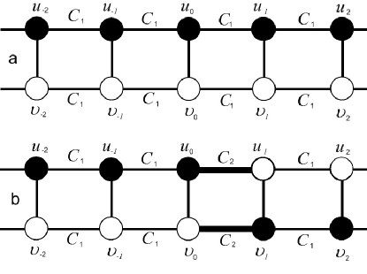
Figure 1: (a) A schematic of the chain of $\mathcal{PT}$-symmetric couplers composed of waveguides with gain and loss, which are designated by dark and bright circles, respectively. (b) The model with the domain wall, created by inverting gain and loss in a half of the chain.

III Analytical results

First, we consider the wave propagation in the array without the DW. The corresponding solution to Eq. (10) in looked for as

$$\left\{\begin{array}[]{c}u_{n}\\ v_{n}\end{array}\right\}=\left\{\begin{array}[]{c}e^{i\delta}\\ 1\end{array}\right\}\exp[i(kn-\omega z)],$$ (15)

where wavenumber $k$ may be complex, while frequency $\omega$ is real. Substituting Eq. (15) into Eq. (10), one finds the high-frequency (HF) and low-frequency (LF) branches of the dispersion relation for the linear waves, denoted by subscripts $h$ and $l$, respectively:

$$\omega_{h} = 2C_{1}\left(1-\frac{e^{ik}+e^{-ik}}{2}\right)-\cos\delta_{h},$$

$$\sin\delta_{h} = -\gamma,\quad\cos\delta_{h}=-\sqrt{1-\gamma^{2}},$$ (16)

$$\omega_{l} = 2C_{1}\left(1-\frac{e^{ik}+e^{-ik}}{2}\right)-\cos\delta_{l},$$

$$\sin\delta_{l} = -\gamma,\quad\cos\delta_{l}=\sqrt{1-\gamma^{2}}.$$ (17)

In particular, for $k=i\kappa$ with real $\kappa$ we obtain an exponential-wave (EW) solution to Eq. (10), while $k=i\kappa+\pi$ gives rise to a staggered exponential-wave (SEW) one. Continuous-wave (CW) solutions correspond to $k=\kappa$, i.e., real wavenumbers. Only these three types of the waves admit real frequencies $\omega$, which, in addition, requires that the gain/loss coefficient must be smaller than the constant of the coupling between the amplified and dissipative waveguides in each $\mathcal{PT}$ element, i.e.,

$$|\gamma|\leq 1.$$ (18)

An example of the spectrum determined by Eqs. (16) and (17) is presented in Fig. 2. In the EW region, $-\infty<\kappa<0$, $\omega_{h}(i\kappa)$ and $\omega_{l}(i\kappa)$ are plotted. The range of $0\leq\kappa\leq\pi$ corresponds to the CW solutions, where we show the frequencies as $\omega_{h}(\kappa)$ and $\omega_{l}(\kappa)$. At $\kappa>\pi$, we have the SEW region, in which the branches of the dispersion relation are plotted as $\omega_{h}(\pi+i[\kappa-\pi])$ and $\omega_{l}(\pi+i[\kappa-\pi])$.

Figure 2: Spectrum of the array without the domain wall, obtained from Eq. (10) for $C_{1}=2$, $\gamma=0.5$. The HF and LF branches, $\omega_{h}$ and $\omega_{l}$, are defined by Eqs. (16),(17), with $k=i\kappa$ for $-\infty<\kappa<0$ (the EW region), $k=\kappa$ for $0\leq\kappa\leq\pi$ (the CW region), and $k=\pi+i(\kappa-\pi)$ for $\pi<\kappa<\infty$ (the SEW region).

Now we proceed to the scattering of linear waves on the DW, within the framework of Eqs. (11)-(14). To this end, we consider an incident wave, with frequency $\omega_{I}$ (and the intensity set equal to $1$), which approaches the DW from the left. Only the case when the incident wave belongs to the LF branch is studied below in an explicit form, as the case of the HF incident wave can be considered similarly.

We look for the scattering solution to Eqs. (11)-(14) as follows:

$$\left\{\begin{array}[]{c}u_{n}\\ v_{n}\end{array}\right\}=e^{i(k_{l}n-\omega_{I}z)}\left\{\begin{array}[]{c}e^{i\delta_{l}}\\ 1\end{array}\right\}$$ (23)

$$+R_{h}e^{i(-k_{h}n-\omega_{I}z)}\left\{\begin{array}[]{c}e^{i\delta_{h}}\\ 1\end{array}\right\}+R_{l}e^{i(-k_{l}n-\omega_{I}z)}\left\{\begin{array}[]{c}e^{i\delta_{l}}\\ 1\end{array}\right\},$$ (28)

for $n\leq 0$, and

$$\left\{\begin{array}[]{c}u_{n}\\ v_{n}\end{array}\right\} = T_{h}e^{i(k_{h}n-\omega_{I}z)}\left\{\begin{array}[]{c}1\\ e^{i\delta_{h}}\end{array}\right\}$$ (36)

$$+T_{l}e^{i(k_{l}n-\omega_{I}z)}\left\{\begin{array}[]{c}1\\ e^{i\delta_{l}}\end{array}\right\},$$

for $n\geq 1$. Here the characteristic of the plane-wave components of the solution are $\sin\delta_{l}=\sin\delta_{h}=-\gamma$, $\cos\delta_{l}=-\cos\delta_{h}=\sqrt{1-\gamma^{2}}$, and $k_{h}$, $k_{l}$ are to be found from Eqs. (16) and Eqs. (17), respectively, where we set $\omega_{h}=\omega_{l}=\omega_{I}$.

Amplitudes $R_{l},\,T_{l}$ and $R_{h},\,T_{h}$, defined in expressions (23) and (36) are complex reflection and transmission coefficients for the LF and HF waves. Substituting these expressions into Eqs. (11)-(14), we obtain

$$R_{l} = \frac{e^{ik_{l}}}{D}\biggl{\{}e_{2}\,(e_{3}-1)+(1-\gamma^{2})\Bigl{[}e_{1}-2e^{2ik_{l}}$$

$$+ e_{3}(e_{1}+4(e^{ik_{h}}-1)-2e_{3})-\overline{C}^{2}\left(1-e_{1}+e_{3}\right)^{2}$$

$$+ \overline{C}\left(1-e^{ik_{l}}\right)^{2}\left(1-e^{ik_{h}}\right)\left(1-3e^{ik_{h}}\right)\Bigr{]}\biggr{\}},$$

$$R_{h} = \frac{e^{ik_{h}}}{D}\left(1-e^{2ik_{l}}\right)\,e_{2}\,\gamma\,(\gamma+i\sqrt{1-\gamma^{2}}),$$

$$T_{l} = \frac{1}{D}\left(-1+e^{2ik_{l}}\right)\left(-1+e^{ik_{h}}\right)\times$$

$$\left[-2e^{ik_{h}}+\overline{C}\left(-1+e^{ik_{h}}\right)\right]\sqrt{1-{\gamma}^{2}},$$

$$T_{h} = -\frac{1}{D}\left(e^{2ik_{l}}-1\right)\left(e_{1}-2e_{3}+{\overline{C}}(e_{3}-e_{1}+1)\right)\times$$ (37)

$$\gamma\sqrt{1-\gamma^{2}}\left(\gamma+i\,\sqrt{1-{\gamma}^{2}}\right)$$

where we define

$$D\equiv{e_{2}}^{2}-\left(1-{\gamma}^{2}\right)\biggl{\{}{e_{1}}^{2}-4e_{3}(e_{1}-e_{3})$$

$$+{\overline{C}}(e_{3}-e_{1}+1)\left[2e_{1}-4e_{3}+{\overline{C}}(e_{3}-e_{1}+1)\right]\biggr{\}},$$ (38)

$$\overline{C} \equiv C_{1}/C_{2},\quad e_{1}\equiv e^{ik_{h}}+e^{ik_{l}},$$ (39)

$$e_{2} \equiv e^{ik_{l}}-e^{ik_{h}},\quad e_{3}\equiv e^{i\,(k_{h}+k_{l})}.$$ (40)

The so obtained reflection and transmission coefficients can be analyzed for the LF incident wave of any of the three types, EW, CW, or SEW. As seen from Eqs. (23) and (36), the incident wave of the LF type generates, generally speaking, both LF and HF reflected and transmitted wave components, whose frequencies are identical to $\omega_{I}$.

We start by considering two examples, which are designated in Fig. 2. Taking $\omega_{I}=\omega_{I}^{\ast}$, we conclude that both $k_{h}=\kappa_{h}^{\ast}$ and $k_{l}=\kappa_{l}^{\ast}$ are in the CW region, meaning that the reflected and transmitted HF and LF waves are all of CW type (here, the asterisk does not stand for the complex conjugate). On the other hand, for $\omega_{I}=\omega_{I}^{\ast\ast}$ we have $k_{h}=-i\kappa_{h}^{\ast\ast}$ and $k_{l}=\kappa_{l}^{\ast\ast}$, meaning that the incident wave is the LF of the CW type, while the reflected and transmitted ones have the HF and LF components of the EW and CW types, respectively.

Care should be taken as concerns the choice of the sign in front of imaginary part of $k_{h}$ and $k_{l}$ for the EW. For the plus (minus) sign, the reflected and transmitted waves of the EW type exponentially decrease (increase) with the increase of the distance from the DW. Both cases are physically meaningful in the $\mathcal{PT}$ system, but in the following we focus only on the evanescent (exponentially decaying) EWs.

Several generic examples of the wave-intensity profiles are present in Fig. 3 in the array of couplers for different frequencies of the incident wave, $\omega_{I}$, which are chosen with regard to the dispersion relation displayed in Fig. 2. As mentioned above, the LF incident wave generates reflected and transmitted waves belonging to the HF and LF branches, with the same frequency $\omega_{I}$. The following four cases are present in Fig. 3: (a) $\omega_{I}=-1$, with $k_{h}=0.931843\,i$, $k_{l}=0.258102\,i$, hence the incident wave is the EW of the LF type, the corresponding HF and LF components also being EWs [see Fig. 3 (a), where the logarithmic scale is used on the vertical axis]. The intensity of the incident wave increases with distance form the DW, while the reflected and transmitted waves are evanescent. (b) $\omega_{I}=0.5$, with $k_{h}=0.424603\,i$, $k_{l}=0.851981$, hence the incident LF wave is a CW, while the reflected and transmitted waves include LF CW and HF evanescent component, the latter rapidly decaying with the distance from the defect [Fig. 3(b)]. (c) $\omega_{I}=6$, with $k_{h}=1.85823$, $k_{l}=2.36958$, in which case all the waves are of the CW type [Fig. 3 (c)]. (d) $\omega_{I}=7.5$, with $k_{h}=2.28961$, $k_{l}=\pi+0.424603\,i$, which makes the incident LF wave an SEW, while the reflected and transmitted waves include the HF CW and LF SEW terms [see Fig. 3 (d), where the logarithmic scale is again used on the vertical axis].

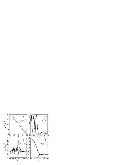
Figure 3: Examples of solutions of the scattering problem in the array of couplers for $C_{1}=2$, $C_{2}=1$, $\gamma=0.5$, and different values of the incident-wave’s frequency, $\omega_{I}$. (a) The incident low-frequency exponential wave excites the high-frequency evanescent wave, with $\omega_{I}=-1$, $k_{h}=0.931843\,i$, $k_{l}=0.258102\,i$. (b) The incident low-frequency CW excites a high-frequency exponential wave, with $\omega_{I}=0.5$, $k_{h}=0.424603\,i$, $k_{l}=0.851981$. (c) The incident low-frequency CW excites a high-frequency CW, with $\omega_{I}=6$, $k_{h}=1.85823$, $k_{l}=2.36958$. (d) The incident low-frequency staggered exponential wave excites a high-frequency CW, with $\omega_{I}=7.5$, $k_{h}=2.28961$, $k_{l}=\pi+0.424603\,i$. Dots and open circles show $|u_{n}|^{2}$ and $|v_{n}|^{2}$, respectively.

Note that, at

$$\sqrt{1-\gamma^{2}}>2C_{1},$$ (41)

the splitting between the LF and HF branches in Fig. 2 becomes so large that their CW regions do not have common frequencies. Under this condition, the case presented in Fig. 3(c), with all the wave components being of the CW type, is impossible. In terms of $\omega_{\min}=\sqrt{1-\gamma^{2}}$ and $\omega_{\max}=4C_{1}-\sqrt{1-\gamma^{2}}$, which are the smallest and the largest frequencies of the HF and LF branches in the CW region (see 2), condition (41) is tantamount to $\omega_{\max}<\omega_{\min}$.

In the following we take $C_{1}\geq 0.5$, which rules out condition (41) for all $0\leq\gamma<1$. We thus always include the possibility of having all the reflected and transmitted waves of the CW type, excited by the incident LF CW.

In the following Section we present the analysis of the transmission and reflection coefficients as functions of parameters of the system, assuming, as said above, $\omega_{\min}<\omega_{\max}$, and focusing on the range of the incident-wave’s frequency $\omega_{\min}<\omega_{I}<\omega_{\max}$, when this wave is of the most relevant CW type. Further, it is convenient to define the normalized frequency,

$$\omega_{I}^{\prime}=\frac{\omega_{I}-\omega_{\min}}{\omega_{\max}-\omega_{\min},}$$ (42)

so that $\omega_{I}^{\prime}=0$ at $\omega_{I}=\omega_{\min}$, and $\omega_{I}^{\prime}=1$ at $\omega_{I}=\omega_{\max}$.

IV Transmission and reflection coefficients

Here we analyze the transmission and reflection coefficients for the LF incident wave, given by Eq. (37) and Eq. (38), varying parameters $\gamma$, $C_{1}$, and $\overline{C}\equiv C_{1}/C_{2}$. As mentioned above, we consider only the case of the CW incident wave as the most natural one. Then, two possibility may be expected, with the incident LF wave exciting either HF-EW or HF-CW.

It is useful to study first the case with no gain and loss, $\gamma=0$. Under this condition, Eq. (37) reduces to

$$R_{l} = \frac{(\overline{C}-1)e^{ik_{l}}(e^{ik_{l}}-1)}{\overline{C}(e^{ik_{l}}-1)-2e^{ik_{l}}},$$

$$R_{h} = 0,$$

$$T_{l} = -\frac{1+e^{ik_{l}}}{\overline{C}(e^{ik_{l}}-1)-2e^{ik_{l}}},$$

$$T_{h} = 0.$$ (43)

From here, we immediately arrive at the conclusion that the LF incident wave excites only the LF reflected and transmitted waves, satisfying condition $|R_{l}|^{2}+|T_{l}|^{2}=1$ due to the energy conservation. Thus, the excitation of the HF reflected and transmitted waves by the LF input is a specific effect of the $\mathcal{PT}$ system, due to the presence of the gain and loss in it. Expressions for $R_{l}$ and $T_{l}$ in Eqs. (43) become singular, with a vanishing denominator, only when $\overline{C}=1$ and $k_{l}=\pi$, which means the absence of the DW in the system (in which case $T_{l}=1$ and $R_{l}=0$). Figure 4 displays $|R_{l}|^{2}$ and $|T_{l}|^{2}$ as functions of $\omega_{I}$ for parameters $\gamma=0$ and $\overline{C}=2$.

Figure 4: $|R_{l}|^{2}$ (the thick line) and $|T_{l}|^{2}$ (the thin line) as functions of $\omega_{I}$ in the case of the incident low-frequency CW for $C_{1}=2$, $C_{2}=1$, and $\gamma=0$ (no gain and loss). In this case, the high-frequency waves are not excited by the low-frequency input ($R_{h}=0$, $T_{h}=0$).

In the presence of the gain and loss ($\gamma>0$) the solution of the scattering problem for the LF incident wave contains $R_{h},T_{h}\neq 0$, i.e., the HF components are excited. Note, however, that $R_{h}=T_{h}=T_{l}$ at $k_{l}=0$ or $k_{l}=\pi$, i.e., at the borders of the considered range of the incident-wave’s frequency, $\omega_{I}$. Also, $T_{l}=0$ if $k_{h}=0$ or $\overline{C}=2/(1-e^{-ik_{h}})$ (the latter is possible in the SEW region, which is not under consideration here).

We now fix $\gamma=0.5$, $C_{1}=2$, and plot the (typical) results, produced by Eqs. (37) for $\overline{C}=2$, $\overline{C}=1$, and $\overline{C}=0.5$.

Figure 5 shows that, at $\overline{C}=2$, all four reflection and transmission coefficients have finite maxima close to the point $\omega_{I}^{\prime}=0.001$ ($\omega_{I}=0.872$). Note that (a’) and (b’) show blowups of (a) and (b), respectively, in the vicinity of the maxima. Also, $T_{l}$ vanishes at $\omega_{I}^{\prime}=0$ ($\omega_{I}=0.866025$).

Figure 5: Relative intensities of the reflected and transmitted waves as functions of $\omega_{I}^{\prime}$ in the case of the low-frequency incident CW, for $\gamma=0.5$ an $\overline{C}=2$. Thick and thin lines depict $|R_{l}|^{2}$, $|R_{h}|^{2}$ in (a) and $|T_{l}|^{2}$, $|T_{h}|^{2}$ in (b), respectively. (a’) and (b’) are the blowups of (a) and (b), respectively.

For $\overline{C}=1$, the reflection and transmission coefficients are presented in Fig. 6. All four coefficients diverge at $\omega_{I}^{\prime}=0.0022$ ($\omega_{I}=0.88$ ) and $\omega_{I}^{\prime}=0.999$ ($\omega_{I}=7.1225$) because at these two points the denominator $D$ in Eq. (37), which is common for all coefficients, vanishes. On (a’),(b’) we show the blowups of (a),(b) for the maxima close to $\omega_{I}^{\prime}=0$, while in (a”),(b”) for the maxima close to $\omega_{I}^{\prime}=1$. The coefficient $T_{l}$ drops to zero at $\omega_{I}^{\prime}=0$ ($\omega_{I}=0.866$).

Figure 6: Same as in Fig. 5, but for $\overline{C}=1$.

For $\overline{C}=0.5$, the reflection and transmission coefficients are displayed in Fig. 7. All the four coefficients have finite maxima at $\omega_{I}^{\prime}=0.00446$ ($\omega_{I}=0.894$), and $T_{l}$ vanishes at $\omega_{I}^{\prime}=0$ ($\omega_{I}=0.86603$).

Figure 7: Same as in Figs. 5 and 6, but for $\overline{C}=0.5$.

The above results can be summarized by saying that for $\overline{C}\neq 1$ all the four reflection and transmission coefficients attain finite maxima at $\omega_{I}^{\prime}$ close (but not equal) to zero. For the special case of $\overline{C}=1$ all four coefficients diverge at $\omega_{I}^{\prime}$ close to zero and close to unity.

It is relevant to note that, if $R_{l}=0$ at a particular value of $\omega_{I}$, then $T_{l}=1$, and, conversely, $R_{l}=1$ if $T_{l}=0$. These cases correspond to the full transmission and full reflection for the LF waves, respectively. However, at $\gamma\neq 0$ the HF reflection and transmission waves are excited too, therefore, in fact, these cases imply not full transmission and reflection, but rather full conversion of LF waves into their HF counterparts.

It is also interesting to consider the effect of amplification of the reflected and transmitted waves, which is possible in the presence of the gain and loss, $\gamma>0$ Miroshnichenko . To this end, we fix $C_{1}=2$ and $C_{2}=1$ and vary the gain/loss parameter within the range of $0\leq\gamma<1$ at fixed $k_{l}$, which leads to the variation of $\omega_{I}$ from $4C_{1}(1-\cos{k_{l}})-1$ to $4C_{1}(1-\cos{k_{l}})$. Accordingly, $k_{h}$ changes too, taking both real and imaginary values. For this case, coefficients $|R_{l}|^{2}$, $|T_{l}|^{2}$, $|R_{h}|^{2}$, and $|T_{h}|^{2}$ are shown versus $\gamma$ in Fig. 8, for $k_{l}=2$ (a) and $k_{l}=1$ (b). Note that $k_{h}$ remains real in (a) for all $\gamma$, while in (b) $k_{h}$ changes from imaginary to real at $\gamma=0.39$. As seen in the figure, in (a) all the reflection and transmission coefficients increase with $\gamma$. On the other hand, in panel (b) they feature additional extrema in a vicinity of the point where $k_{h}$ changes from imaginary to real.

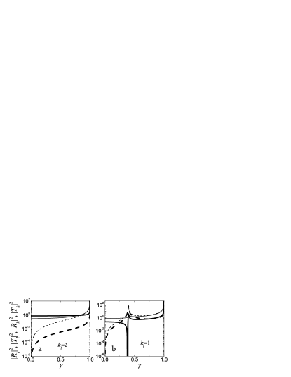
Figure 8: $|R_{l}|^{2}$ (thick line), $|T_{l}|^{2}$ (thin line), $|R_{h}|^{2}$ (dashed thick line), $|T_{h}|^{2}$ (dashed thin line) as functions of $\gamma$ in the case of low-frequency incident CW for $C_{1}=2$, $C_{2}=1$. (a) $k_{l}=2$ with real $k_{h}$, and (b) $k_{l}=1$ with $k_{h}$ changing from imaginary to real at $\gamma=0.39$.

Figure 9: $|R_{l}|^{2}+|R_{h}|^{2}$ and $|T_{l}|^{2}+|T_{h}|^{2}$ (thick and thin lines, respectively) as functions of $\omega_{I}^{\prime}$ in the case of low-frequency incident CW for $C_{1}=2$, $C_{2}=1$, and $\gamma=0.01$ (a), $\gamma=0.5$ (b), $\gamma=0.9$ (c), $\gamma=0.999$ (d) Note that the vertical scale is logarithmic.

The amplification of the reflected and transmitted waves can be defined in terms of their total intensities. Thus, in the case of the incident LF CW, when both reflected and transmitted HF waves are of CW type, the amplification of reflection and transmission takes place when $|R_{l}|^{2}+|R_{h}|^{2}>1$ and $|T_{l}|^{2}+|T_{h}|^{2}>1$, respectively (as shown in Fig. 9). We notice that the range of the incident-wave’s frequency, $\omega_{I}$, where the amplification occurs, increases with $\gamma$. Also note that in Fig. 9 (a) the reflection and transmission coefficients feature sharp maxima in a vicinity of $\omega_{I}^{\prime}=0$. In the limit $\gamma=0$, as it has been already mentioned, the system becomes conservative and these maxima disappear.

V Conclusions

We have studied the scattering of linear waves on a domain wall introduced into a waveguide array composed of $\mathcal{PT}$-symmetric waveguide pairs. Such arrays support the propagation of HF (high-frequency) and LF (low-frequency) waves. Considering incident LF waves of various types (continuous waves or unstaggered and staggered exponential waves), we have derived the corresponding reflection and transmission coefficients and analyzed their dependence on the system parameters. The case of the HF incident wave can be analyzed similarly.

We have found that the LF incident wave generates both LF and HF reflected and transmitted waves, provided that the gain and loss are present ($\gamma>0$). We also demonstrated that both reflected and transmitted waves can be substantially amplified, provided that the gain $\gamma>0$ is present. The range of the incident-wave’s frequency where the amplification takes place expands with the increase of $\gamma$.

Our results suggest that the use of $\mathcal{PT}$-symmetric elements in waveguide arrays offers various possibilities for manipulations of optical signals in photonic lattices. It may be interesting to add nonlinearity to the system. In addition to the formation of solitons we , the nonlinearity may give rise to spontaneous symmetry breaking Miroshnichenko . Obviously, these effects may strongly affect the scattering problem. Finally, a challenging problem is to extend the analysis to the case of two-dimensional $\mathcal{PT}$-invariant networks.

References

- (1) C. M. Bender, S. Boettcher, Phys. Rev. Lett. 80, 5243 (1998); C. M. Bender, D.C. Brody, H. F. Jones, ibid. 89, 270401 (2002); C. M. Bender, D.C. Brody, and H. F. Jones, ibid. 92, 119902(E) (2004); C. M. Bender, Rep. Progr. Phys. 70, 947 (2007).
- (2) A. Ruschhaupt, F. Delgado, and J. G. Muga, J. Phys. A 38, L171 (2005); R. El-Ganainy, K. G. Makris, D. N. Christodoulides, and Z. H. Musslimani, Opt. Lett. 32, 2632 (2007).
- (3) M. V. Berry, J. Phys. A 41, 244007 (2008); K. G. Makris, R. El-Ganainy, D. N. Christodoulides, and Z. H. Musslimani, Phys. Rev. Lett. 100, 103904 (2008); S. Klaiman, U. Günther, and N. Moiseyev, ibid. 101, 080402 (2008); S. Longhi, ibid. 103, 123601 (2009); K. G. Makris, R. El-Ganainy, D. N. Christodoulides, and Z. H. Musslimani, Phys. Rev. A 81, 063807 (2010); S. Longhi Phys. Rev. A 82, 031801(R)(2010); Y. N. Joglekar, D. Scott, M. Babbey, and A. Saxena, ibid. 82, 030103(R) (2010); G. L. Giorgi, Phys. Rev. B 82, 052404 (2010); C. T. West, T. Kottos, and T. Prosen, Phys. Rev. Lett. 104, 054102 (2010); K. Li and P. G. Kevrekidis, Phys. Rev. E 83, 066608 (2011); Z. Lin, H. Ramezani, T. Eichelkraut, T. Kottos, H. Cao, and D. N. Christodoulides, Phys. Rev. Lett. 106, 213901 (2011); C. He, M.-H. Lu, X. Heng, L. Feng, and Y.-F. Chen, Phys. Rev. B 83, 075117 (2011).
- (4) A. A. Sukhorukov, Z. Xu, and Yu. S. Kivshar, Phys. Rev. A 82, 043818 (2010); R. Driben and B. A. Malomed, Stability of solitons in -symmetric couplers, Opt. Lett., in press.
- (5) S. V. Dmitriev, A. A. Sukhorukov, and Yu. S. Kivshar, Opt. Lett. 35, 2976 (2010).
- (6) A. E. Miroshnichenko, B. A. Malomed, and Yu. S. Kivshar, Phys. Rev. A 84, 012123 (2011).
- (7) S. V. Dmitriev, S. V. Suchkov, A. A. Sukhorukov, Yu. S. Kivshar, Phys. Rev. A 84, 013833 (2011).
- (8) S. V. Suchkov, B. A. Malomed, S. V. Dmitriev, and Yu. S. Kivshar, Phys. Rev. E 84, 046609 (2011).
- (9) A. Guo, G. J. Salamo, D. Duchesne, R. Morandotti, M. Volatier-Ravat, V. Aimez, G. A. Siviloglou, and D. N. Christodoulides, Phys. Rev. Lett. 103, 093902 (2009); C. E. Ruter, K. G. Makris, R. El-Ganainy, D. N. Christodoulides, M. Segev, and D. Kip, Nature Physics 6, 192 (2010); J. Schindler, A. Li, M. C. Zheng, F. M. Ellis, and T. Kottos Phys. Rev. A 84, 040101(R) (2011).
- (10) A. F. Sadreev and I. Rotter, J. Phys. A: Math. Gen. 36, 11413 (2003); G. L. Celardo, A. M. Smith, S. Sorathia, V. G. Zelevinsky, R. A. Sen’kov, and L. Kaplan, Phys. Rev. B 82, 165437 (2010).
- (11) V. V. Sokolov and V. G. Zelevinsky, Nucl. Phys. B 202, 10 (1988); Nucl. Phys. A 504, 562 (1989); Ann. Phys. 216, 323 (1992); G. L. Celardo and L. Kaplan, Phys. Rev. B 79, 155108 (2009).