Anisotropy-induced Fano resonance

Abstract

An optical Fano resonance, which is caused by birefringence control rather than frequency selection, is discovered. Such birefringence-induced Fano resonance comes with fast-switching radiation. The resonance condition $\varepsilon_{t}<1/\varepsilon_{r}$ is revealed and a tiny perturbation in birefringence is found to result in a giant switch in the principal light pole induced near surface plasmon resonance. The loss and size effects upon the Fano resonance have been studied Fano resonance is still pronounced, even if the loss and size of the object increase. The evolutions of the radiation patterns and energy singularities illustrate clearly the sensitive dependence of Fano resonance upon the birefringence.

PACS numbers: 78.20.Fm,42.65.Es,46.40.Ff,78.67.Bf

Light scattering by a small particle is one of the most fundamental problems in electrodynamics and potential applications in information processing, nanotechnologies and engineering. The essence of extraordinary light scattering is the localized surface plasmon which is oscillating with the frequency of the incident wave Tsai . For particles with the size much smaller than the incident wavelength, Rayleigh approximation can be adopted Hulst. Nonetheless, recent studies show that for small particle with weak dissipation near plasmon resonance frequencies, anomalous light scattering takes place with unexpected features, e.g., sharp giant optical resonances with inverse hierarchy, unusual frequency and particle size dependence, and complicated near-field energy circulation Tribelsky ; Luk'yanchuk1 ; Qiu . Recently, a lot of studies were related to the resonances in plasmonic nanostructures Maier_ACS09 ; Giessen09 ; Tribelsky2 ; Boris_NM , coherent nanocavities Maier_NL , and metallic films Stockman ; Garcia . However, they were discussed for isotropic materials or elements, and also Fano resonance was observed versus the fine tuning of frequency.

In this letter, we provide a new paradigm to realize Fano resonance via the birefringence (anisotropy) of a single particle, instead of controlling frequency. This novel resonant mechanism may be a new paradigm for sensitive optical identification of molecular groups, calculation of heating, radiation pressure and trapping. The anisotropy is found to be able to tailor the surface plasmon resonance and induce additional plasmonic resonances. It is thus revealed that birefringence-induced Fano resonance occurs to the anisotropic rod and its radiation pattern is affected by the subtle perturbation of the rod’s birefringence. We also look into the near field where Poynting bifurcation and vortex analysis are investigated against the birefringence-induced Fano resonant cases. Note that the anisotropic parameters are homogeneous, i.e., position-independent, which is in contrast to the parameters of a cloak Pendry . Here we would like to consider the homogeneous rod with constant radial anisotropy in both $\mathord{\buildrel{\lower 3.0pt\hbox{$\scriptscriptstyle\leftrightarrow$}}\over{\varepsilon}}$ and $\mathord{\buildrel{\lower 3.0pt\hbox{$\scriptscriptstyle\leftrightarrow$}}\over{\mu}}$, i.e., they are diagonal in cylindrical coordinates with values $\varepsilon_{r}(\mu_{r})$ in the radial ($\mathord{\buildrel{\lower 3.0pt\hbox{$\scriptscriptstyle\rightharpoonup$}}\over{r}}$) direction and $\varepsilon_{t}(\mu_{t})$ in the other two directions ($\mathord{\buildrel{\lower 3.0pt\hbox{$\scriptscriptstyle\rightharpoonup$}}\over{\theta}}$ and $\mathord{\buildrel{\lower 3.0pt\hbox{$\scriptscriptstyle\rightharpoonup$}}\over{z}}$). Actually, such birefringence can be realized by graphitic multishells Lucas or stratified mediums Sten , and in practice, it has been found in phospholipid vesicle systems Lange ; Peterlin and in cell membranes containing mobile charges Sukhorukov ; Ambjornsson .

The magnetic field only exists in the z-direction. The constitutive tensors of the relative permittivity and permeability are expressed as $\mathord{\buildrel{\lower 3.0pt\hbox{$\scriptscriptstyle\leftrightarrow$}}\over{\varepsilon}}=\varepsilon_{r}\mathord{\buildrel{\lower 3.0pt\hbox{$\scriptscriptstyle\rightharpoonup$}}\over{r}}\mathord{\buildrel{\lower 3.0pt\hbox{$\scriptscriptstyle\rightharpoonup$}}\over{r}}+\varepsilon_{t}\mathord{\buildrel{\lower 3.0pt\hbox{$\scriptscriptstyle\rightharpoonup$}}\over{\theta}}\mathord{\buildrel{\lower 3.0pt\hbox{$\scriptscriptstyle\rightharpoonup$}}\over{\theta}}+\varepsilon_{t}\mathord{\buildrel{\lower 3.0pt\hbox{$\scriptscriptstyle\rightharpoonup$}}\over{z}}\mathord{\buildrel{\lower 3.0pt\hbox{$\scriptscriptstyle\rightharpoonup$}}\over{z}}$ and $\mathord{\buildrel{\lower 3.0pt\hbox{$\scriptscriptstyle\leftrightarrow$}}\over{\mu}}=\mu_{r}\mathord{\buildrel{\lower 3.0pt\hbox{$\scriptscriptstyle\rightharpoonup$}}\over{r}}\mathord{\buildrel{\lower 3.0pt\hbox{$\scriptscriptstyle\rightharpoonup$}}\over{r}}+\mu_{t}\mathord{\buildrel{\lower 3.0pt\hbox{$\scriptscriptstyle\rightharpoonup$}}\over{\theta}}\mathord{\buildrel{\lower 3.0pt\hbox{$\scriptscriptstyle\rightharpoonup$}}\over{\theta}}+\mu_{t}\mathord{\buildrel{\lower 3.0pt\hbox{$\scriptscriptstyle\rightharpoonup$}}\over{z}}\mathord{\buildrel{\lower 3.0pt\hbox{$\scriptscriptstyle\rightharpoonup$}}\over{z}}$ respectively in cylindrical coordinates, where $\varepsilon_{r}(\mu_{r})$ and $\varepsilon_{t}(\mu_{t})$ stand for the permittivity (permeability) elements corresponding to the electric- and magnetic- field vector normal to and tangential to the local optical axis, respectively. The time dependence $e^{-i\omega t}$ is assumed. We rely on Mathematica^TM to produce all the results throughout.

For the TE mode, we have the wave equation

$$\frac{1}{r}\left[{\frac{\partial}{{\partial r}}\left({\frac{r}{{\varepsilon_{t}}}\frac{{\partial H_{z}}}{{\partial r}}}\right)}\right]+\frac{1}{{r^{2}}}\frac{\partial}{{\partial\theta}}\left({\frac{1}{{\varepsilon_{r}}}\frac{{\partial H_{z}}}{{\partial\theta}}}\right)+k_{0}^{2}\mu_{t}H_{z}=0.$$ (1)

The local field solutions in the inner and outer region of the wire can be described as $H_{z}^{in}=\sum\limits_{m=-\infty}^{\infty}{i^{m}A_{m}J_{m^{\prime}}(kr)e^{im\theta}}$ and $H_{z}^{out}=\sum\limits_{m=-\infty}^{\infty}{i^{m}[J_{m}(k_{0}r)+B_{m}H_{m}^{(1)}(k_{0}r)]e^{im\theta}}$, respectively, where $k=k_{0}\sqrt{\varepsilon_{t}\mu_{t}}$ and $k_{0}=\omega\sqrt{\varepsilon_{0}\mu_{0}}$. Note that the Bessel function index m’, i.e., $m^{\prime 2}=m^{2}\varepsilon_{t}/\varepsilon_{r}$ is no longer a conventional integer, which is different from the uniaxial material considered in Bohren . Under TE (or TM) incidence, the uniaxial material in Bohren is actually isotropic, while our birefringent material is defined in cylindrical coordinate and is not isotropic under TE (or TM) incidence Lucas ; Sten ; Lange ; Peterlin ; Sukhorukov ; Ambjornsson . To solve the scattering problem, the scattering coefficient $B_{m}$ now becomes the most important issue:

$$B_{m}=-\frac{\sqrt{\varepsilon_{t}\mu_{t}}J_{m^{\prime}}(\sqrt{\varepsilon_{t}\mu_{t}}q)J_{m}^{{}^{\prime}}(q)-\mu_{t}J_{m}(q)J_{m^{\prime}}^{{}^{\prime}}(\sqrt{\varepsilon_{t}\mu_{t}}q)}{{\sqrt{\varepsilon_{t}\mu_{t}}J_{m^{\prime}}(\sqrt{\varepsilon_{t}\mu_{t}}q)H_{m}^{(1)^{\prime}}(q)-\mu_{t}J_{m^{\prime}}^{{}^{\prime}}(\sqrt{\varepsilon_{t}\mu_{t}}q)}H_{m}^{(1)}(q)}$$ (2)

where the prime denotes the derivative with respect to the argument and the size parameter is $\emph{q}=k_{0}a$. It is evident that $B_{m}$ reduces to the isotropic case by replacing $\varepsilon_{r}(\varepsilon_{t})$ and $\mu_{r}(\mu_{t})$ with $\varepsilon$ and $\mu$, respectively Bohren .

Note that the “effective” permittivity and permeability can be isotropic even for a radially birefringent object Fung . In search of the effective response for such a birefringent cylinder, one assumes that the rod with radial anisotropy is embedded in an effective medium with isotropic effective permittivity $\varepsilon_{eff}$ and permeability $\mu_{eff}$ and when no scattering arises, the search stops, i.e., “effective” parameters are found. In this sense, we replace $\varepsilon_{0}$ and $\mu_{0}$ by $\varepsilon_{0}\varepsilon_{eff}$ and $\mu_{0}\mu_{eff}$, and they can be determined. By considering the equivalence to the isotropic case for $q\to 0$, the surface resonant condition tends to be $\varepsilon_{eff}=\sqrt{\varepsilon_{r}}\sqrt{\varepsilon_{t}}=-1$, i.e., $\varepsilon_{t}=1/\varepsilon_{r}$ for negative $\varepsilon_{r}$.

To explain the optical resonances numerically, let us present the amplitude

$$B_{m}=-\frac{{\Re_{m}}}{{\Re_{m}+i\Im_{m}}}$$ (3)

by separating the real and imaginary parts, then we have

$$\Re_{m}=\sqrt{\varepsilon_{t}\mu_{t}}J_{m^{\prime}}(\sqrt{\varepsilon_{t}\mu_{t}}q)J_{m}^{\prime}(q)-\mu_{t}J_{m}(q)J_{m^{\prime}}^{\prime}(\sqrt{\varepsilon_{t}\mu_{t}}q)$$ (4)

$$\Im_{m}=\sqrt{\varepsilon_{t}\mu_{t}}J_{m^{\prime}}(\sqrt{\varepsilon_{t}\mu_{t}}q)Y_{m}^{\prime}(q)-\mu_{t}J_{m^{\prime}}^{\prime}(\sqrt{\varepsilon_{t}\mu_{t}}q)Y_{m}(q)$$ (5)

where $Y_{m}$ is the Neumann function. The exact optical resonance corresponds to the situation when $\Im_{m}=0$, which leads to $\left|{B_{m}}\right|=1$. For simplicity, the material is assumed to be non-magnetic, i.e., $\mu_{t}=1$.

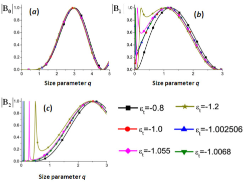
Figure 1: (Color online) Analysis of resonant conditions and dominant modes versus size parameter q for monopole resonance m=0 (a); dipole resonance m=1 (b), and quadrupole resonance m=2 (c). (a-c) show how the new additional resonances will be induced by the tiny perturbation in birefringence for high-order resonances (e.g., dipole, quadrupole, etc). Here we keep $\varepsilon_{r}=-1$, and $\delta=\varepsilon_{t}-\varepsilon_{r}$ which serves the measure of birefringence. Hence $\varepsilon_{t}=-1$ (i.e., $\delta=0$) corresponds to the isotropic situation.

In Fig. 1(a), it indicates that there is no surface resonance at small q and the maximum magnitude of $B_{0}$ always occurs in the vicinity of $q\approx 2.8$ no matter how the transversal permittivity $\varepsilon_{t}$ deviates from the radial permittivity $\varepsilon_{r}$. Nevertheless, new resonances will be excited in higher-order modes (e.g., dipolar, quadrupolar, etc) as shown in Figs. 1(b,c) at small size parameter q. In Fig. 1(c), one can see the isotropic case (the red line), i.e., $\varepsilon_{t}=-1=\varepsilon_{r}$, does not have the additional optical surface resonance at very small q. Under the resonant condition $\varepsilon_{t}<\varepsilon_{r}$, Figs. 1(b,c) reveal that a slight deviation from the isotropic case ($\varepsilon_{t}=-1$), i.e., the perturbation of birefringence $\delta\neq 0$, will give rise to a new surface resonance for small particles. When $\varepsilon_{t}$ is very closer to $-1$, the additional optical resonance for higher-order modes will be more isolated from the volume resonance (which is still found to be insensitive as the monopole). When $\varepsilon_{t}$ is more deviated from $-1$, the optical resonance will be merging with the volume resonance. Obviously, the case of $\varepsilon_{t}=0.8$ in Fig. 1 does not satisfy the surface resonant condition, so it only possesses a volume resonance. Considering the resonance trajectory, it is not difficult to propose $d\varepsilon_{t}/dq$. Negative (positive) value denotes surface (volume) resonance.

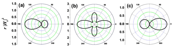
Figure 2: (Color online) Polar diagrams for light intensity versus observation angle $\theta$ associated with Fano resonance and fast-switching radiation pattern. We assume $q=0.1$ and $\varepsilon_{r}=-1$. (a) $\delta=-0.0065$; (b) $\delta=-0.0067835$; (c) $\delta=-0.0071$. The switching radiation pattern versus the change of birefringence has been demonstrated (Media 1).

Strong variations of the total scattered intensity are caused by a tiny change in birefringence. As is shown in Fig. 2, when the parameters $\varepsilon_{r}$ and $\varepsilon_{t}$ fit the condition of the surface plasmon resonance, an equilibrium state with a symmetrical pattern is yielded, and in the vicinity of the equilibrium, the radiation pattern flips fast just because of a tiny perturbation of the birefringence ( here we change $\varepsilon_{t}$ while keeping $\varepsilon_{r}=-1$). With the increase in $\varepsilon_{t}$, more and more light is directed into the forward direction “before” it passes the equilibrium state; but after right passing that symmetrical state, light starts to be directed back into the backward direction, and such switch is quite sensitive to the variation of birefringence.

To reveal the near-field distribution when Fano resonance occurs, we investigate Poynting vector ${\bf S}$ bifurcation and distribution of singularity points which is sensitively altered by the birefringence of the particle. In Fig. 3, we investigate 4 typical situations: 1) no birefringence is present (Fig. 3(a)); 2) birefringent case at equilibrium resonant state (in Fig. 3(c)); 3) birefringent cases “before” and “after” the equilibrium resonant state (in Figs. 3(b,d) respectively). Based on our approach and analysis, the Poynting vector lines and their bifurcations demonstrate various types of singular points: (1) ordinary singularities defined as the zeroes of the vector ${\bf S}$; (2) so-called boundary singular points defined as $S_{r}(r=a,\varphi)=0$. It shows that the ordinary singularities (red dots in Media 2) outside the particle will be shifted further away (out of the plot area) but those inside the particle will be moving towards the center and gradually merging into one common singularity in the center eventually.

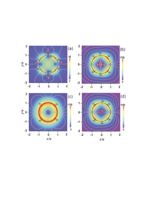
Figure 3: (Color online) Poynting vector $|{\bf S}|$ distribution, lines of Poynting vector ${\bf S}$, and singular points for (a) isotropic cylinder $\delta=0$ and anisotropic ones (b) $\delta=-0.0065$; (c) $\delta=-0.0067835$; (d) $\delta=-0.0071$. Parameters: $q=0.1$ and $\varepsilon_{r}=-1$. In the figures two types of singularities are shown: usual singularities (red points) and boundary singularities (black points at the cylinder boundary). The sensitive dependence of singularities along the change of anisotropy can be seen (Media 2).

The number of boundary singularities keeps unaffected when the object becomes anisotropic, except at the equilibrium resonant state. However, the positions of those boundary singularities will be sensitively dependent on the degree of anisotropy. The points 1b–4b appear for all cases, where $b$ denotes boundary singular points. Points 5b and 6b are more interesting. If no anisotropy exists as in Fig. 3(a), 5b and 6b are located on the crossing points of the object’s boundary and the vertical line passing through the center (0,0). When radial anisotropy is introduced as in Figs. 3(b,d), points 5b and 6b will be shifted away from the centered vertical line. Of particular interest is the situation of Fig. 3(c), where a symmetrical radiation pattern holds in both near and far regions. In such an equilibrium state, points 1b-4b are located symmetrically on the boundary while Points 5b and 6b disappear. It is found that the change of singular points is not continuous in birefringent situations, and points 5b and 6b are either shifted away from the center line or not present (see the black dots in Media 2).

Figure 3(a) also reveals that there are eight normal singularities in the vicinity of the isotropic cylinder (more points exist afar). The points 1–4 (5–8) are situated outside (inside) the cylinder. Birefringent cylinder offers the fundamental distinction: a saddle point arises exactly at the center (0,0). The numbers of singular points become less near a birefringent cylinder, but some points exist outside the ranges of the figures. The singularity investigation gives us more physical insights of how energy is directed and localized, which may be helpful in exploring calculation of heating, radiation pressure and trapping furthermore.

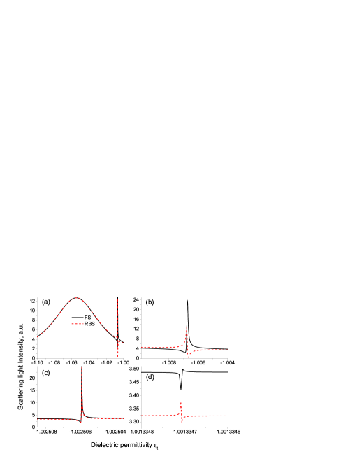
Figure 4: (Color online) The far-field scattering intensity (a.u.) versus transversal permittivity $\varepsilon_{t}$ when $q=0.1$ and $\varepsilon_{r}=-1$. (a) Forward scattering (FS) and radar backscattering (RBS) in the region of $-1.1<\varepsilon_{t}<-1$, i.e., $-0.1<\delta<0$. (b) Asymmetric resonance corresponding to fast-switching radiation pattern near $\varepsilon_{t}\approx-1.0068$ shown in Fig. 3. (c) Symmetric resonance near $\varepsilon_{t}\approx-1.002506$ which leads to almost symmetrical radiation pattern (see the evolution in Media 3). (d) Symmetric resonance near $\varepsilon_{t}\approx-1.0013347$ which is less dominant.

To have a better understanding of the birefringence-induced Fano resonance, we investigate birefringence dependence of the far-field scattering intensity, particularly for forward scattering (FS) and radar backscattering (RBS). In Fig. 4(a), it is clear that there are very sensitive resonances in the narrow region of $-1.01<\varepsilon_{t}<-1$. Specifically, we found three resonances as shown in Fig. 4(b), 4(c) and 4(d), respectively. The fast-switching radiation (i.e., FS and RBS flip over), which attributes to similar Fano resonance in Figs. 2 and 3, is corresponding to the first resonance reported in Fig. 4(b). It can be found in Media 1 that such resonance is quite asymmetric. On the contrary, Media 3 clearly demonstrates that the resonance in Fig. 4(c) is quite symmetric along the change of birefringence near $delta\approx-0.002506$. The additional resonance in Fig. 4(d) appears to be also asymmetric but less dominant compared to the other resonances, which is not discussed herein.

Does it mean that the last sentence above is not true after your recent checks (your previous comments were as below)? If it is still true, i think the current Fig.5 is not 100% targeted to the reviewer’s concern. Fig.5 is great, but presents too much information (without matching discussion) and didn’t selectively address reviewer’s question.

We only need to show two cases (e.g., $\alpha=0.01$ and $\alpha=0.1$) or just only one case $\alpha=0.01$, if we can exactly illustrate the process of first resonance being broadened and one high-order resonance being narrower, and we can tune different $\epsilon_{r}$ to let it pronounce.

The birefringence-induced Fano resonance with extreme sensitivity is presented and can be used for different applications, e.g., data storage and optical recording. For more detailed information, we investigate the both near-field and far field phenomena by using the full-wave approach. The localized field distributions in the vicinity of the resonant condition agrees with the directivity switch in far-field due to the Fano resonance and high-order modes’ interference. Such Fano resonance is found to be existing even when the loss is not negligible or the particle’s size is large. In conclusion, Fano resonances are generated with the condition $\varepsilon_{t}<1/\varepsilon_{r}$, which leads to a giant switch in the principal light pole induced near surface plasmon resonance with a tiny perturbation in birefringence.

Media 1, 2, and 3 are movies, supplied as supplementary files. This work was supported by the National University of Singapore under Grant No. R-263-000-574-133.

References

- (1) W.L. Barnes, A. Dereux, and T.W. Ebbesen, Nature 424, 824 (2003). S.A. Maier et al., Nat. Mater. 2, 229 (2003).
- (2) C. F. Bohren and D. R. Huffman, Absorption and Scattering of Light by Small Particles (Willey, New York, 1983). H. C. Van De Hulst, Light Scattering by Small Particles (Dover, New York, 2000.)
- (3) M. I. Tribelsky and B. S. Luk’yanchuk, Phys. Rev. Lett. 97, 263902 (2006).
- (4) B. S. Luk’yanchuk and V. Ternovsky, Phys. Rev. B 73, 235432 (2006).
- (5) C.-W. Qiu and B.S. Luk’yanchuk, J. Opt. Soc. Am. A 25, 1623 (2008).
- (6) F. Hao et al., ACS Nano 3, 643 (2009).
- (7) N. Liu et al., Nat. Mater. 8, 758 (2009).
- (8) M. I. Tribelsky et al., Phys. Rev. Lett. 100, 043903 (2008).
- (9) B. Luk‘yanchuk et al., Nat. Mater. 9, 707 (2010).
- (10) N. Verellen et al., Nano Lett. 9, 1663 (2009).
- (11) M.I. Stockman, S.V. Faleev, and D.J. Bergman, Phys. Rev. Lett. 87, 167401 (2001).
- (12) F. J. Garcia-Vidal, L. Martin-Moreno, T. W. Ebbesen, and L. Kuipers, Rev. Mod. Phys. 82, 729 (2010).
- (13) J.B. Pendry, D. Schurig, and D.R. Smith, Science 312, 1780 (2006).
- (14) A.A. Lucas, L. Henrard, Ph. Lambin, Phys. Rev. B 49, 2888 (1994).
- (15) J.C.E. Sten, IEEE Trans. Dielectr. Electr. Insul. 2, 360 (1995).
- (16) B. Lange and S.R. Aragon, J. Chem. Phys. 92, 4643 (1990).
- (17) P. Peterlin, S. Svetina, and B. Zeks, J. Phys.: Condens. Matter 19, 136220 (2007).
- (18) V.L. Sukhorukov, G. Meedt, M. Kurschner, U. Zimmermann, J. Electrost. 50, 191 (2001).
- (19) T. Ambjornsson, G. Mukhopadhyay, S.P. Apell, and M. Kall, Phys. Rev. B 73, 085412 (2006).
- (20) L. Gao et al., Phys. Rev. E 78, 046609 (2008). Y. Wu et al., Phys. Rev. B 74, 085111 (2006).