A cluster expansion approach to exponential random graph models

Abstract

The exponential family of random graphs is among the most widely-studied network models. We show that any exponential random graph model may alternatively be viewed as a lattice gas model with a finite Banach space norm. The system may then be treated by cluster expansion methods from statistical mechanics. In particular, we derive a convergent power series expansion for the limiting free energy in the case of small parameters. Since the free energy is the generating function for the expectations of other random variables, this characterizes the structure and behavior of the limiting network in this parameter region.

1 Introduction

Random graphs have been widely studied (see [1, 2] for surveys of recent work) since the pioneering work on the independent case. The first serious attempt was made by Solomonoff and Rapoport [3] in the early 1950s, who proposed the “random net” model in their investigation into mathematical biology. A decade later, Erdős and Rényi [4] independently rediscovered this model and studied it exhaustively, hence the namesake “Erdős-Rényi random graph”. Their construction was straightforward: Take $n$ identical vertices, and connect each pair by undirected edges independently with probability $p$. Many properties of this simple random graph are exactly solvable in the large $n$ limit. Perhaps the most important feature is that it possesses a phase transition: From a low-density, low-$p$ state in which there are few edges to a high-density, high-$p$ state in which an extensive fraction of all vertices are joined together in a single giant component.

The Erdős-Rényi random graph, while illuminating, is a poor model for most real-world networks, as has been argued by many authors [5, 6, 7], and so it has been extended in a variety of ways. To address its unrealistic degree distribution, generalized random graph models such as the configuration model [8] and the multipartite graph model [9] have been developed. However, these models have a serious shortcoming, in that they fail to capture the common phenomenon of transitivity exhibited in social and biological networks of various kinds.

The main hope for progress in this direction seems to lie in formulating a model that incorporates graph structure in more detail. A top candidate is the exponential random graph model, in which dependence between the random edges is defined through certain finite subgraphs, in imitation of the use of potential energy to provide dependence between particle states in a grand canonical ensemble of statistical physics. These exponential models were first studied by Holland and Leinhardt [10] in the directed case, and later developed extensively by Frank and Strauss [11], who related the random graph edges to a Markov random field. More developments are summarized in [12, 13, 14].

The past few years have witnessed a surge of interest in the study of the limiting behavior of exponential random graphs. A major problem in this field is the evaluation of the free energy, a quantity that is crucial for carrying out maximum likelihood and Bayesian inference. A particular motivation for people in the statistical mechanics community to study the free energy is that it provides information on phase transition in these sophisticated models. Many people have made substantial contributions in this area: Häggström and Jonasson [15] examined the phase structure and percolation phenomenon of the random triangle model. Park and Newman [16, 17] constructed mean-field approximations and analyzed the phase diagram for the edge-two-star and edge-triangle models. Borgs et al. [18] established a lower bound on the largest component above the critical threshold for random subgraphs of the $n$-cube. Bollobás et al. [19] showed that for inhomogeneous random graphs with (conditional) independence between the edges, the critical point of the phase transition and the size of the giant component above the transition could be determined under one very weak assumption. Bhamidi et al. [20] focused on the mixing time of the Glauber dynamics and proposed that in the high temperature regime the exponential random graph is not appreciably different from the Erdős-Rényi random graph. Dembo and Montanari [21] discovered that for the Ising model on a sparse graph phase transitions and coexistence phenomena are related to Gibbs measures on infinite trees. Using the emerging tools of graph limits as developed by Lovász and coworkers [22], Chatterjee and Diaconis [23] gave the first rigorous proof of singular behavior in the edge-triangle model. They also suggested that, quite generally, models with repulsion exhibit a transition qualitatively like the solid/fluid transition, in which one phase has nontrivial structure, as distinguished from the “disordered” Erdős-Rényi graphs. Radin and Yin [24] derived the full phase diagram for a large family of $2$-parameter exponential random graph models with attraction and showed that they all contain a first order transition curve ending in a second order critical point (qualitatively similar to the gas/liquid transition in equilibrium materials). Aristoff and Radin [25] considered random graph models with repulsion and proved that the region of parameter space corresponding to multipartite structure is separated by a phase transition from the region of disordered graphs (proof recently improved by Yin [26]).

As is usual in statistical mechanics, we work with a finite probability space, and interpret our results in some more sophisticated limiting sense. We consider general $k$-parameter families of exponential random graphs.

• A complete graph $K_{n}$ on $n$ vertices consists of a vertex set $V_{n}$ ($|V_{n}|=n$) and an edge set $E_{n}$ ($|E_{n}|={n\choose 2}$). A vertex pair $e$ is a two-element subset of $V_{n}$, and the set of all vertex pairs constitute $E_{n}$.

• $\mathcal{G}_{n}$ is the set of simple graphs $G$ on $n$ vertices, where a graph $G$ with vertex set $V(G)=V_{n}$ is simple if its edge set $E(G)$ is a subset of $E_{n}$.

• $H_{1},...,H_{k}$ are pre-chosen finite simple graphs. Each $H_{i}$ has $m_{i}$ vertices ($2\leq m_{i}\leq m$) and $p_{i}$ edges ($1\leq p_{i}\leq p$). In particular, $H_{1}$ is $K_{2}$ (i.e. a single edge).

• A vertex map $f:V(H_{i})\to V(G)$ is a homomorphism if the induced edge map $f_{*}:E(H_{i})\to E_{n}$ sends $E(H_{i})$ into $E(G)$. $t(H_{i},G)$ is the density of graph homomorphisms $H_{i}\to G$:

  $$t(H_{i},G)=\frac{|\text{hom}(H_{i},G)|}{|\text{hom}(H_{i},K_{n})|},$$ (1)

  where the denominator $|\text{hom}(H_{i},K_{n})|=n^{m_{i}}$ counts the total number of mappings from $V(H_{i})$ to $V(G)$.

• $\beta=(\beta_{1},...,\beta_{k})$ are $k$ real parameters. They tune the influence of the pre-chosen graphs $H_{1},...,H_{k}$.

Let $T^{\beta}(G)$ be the weighted sum of graph homomorphism densities $t(H_{i},G)$:

$$T^{\beta}(G)=\sum_{i=1}^{k}\beta_{i}t(H_{i},G).$$ (2)

There is a probability mass function that assigns to every $G$

$$\mathbb{P}_{n}^{\beta}(G)=\exp\left(n^{2}(T^{\beta}(G)-\psi_{n}^{\beta})\right),$$ (3)

where $\psi^{\beta}_{n}$ is the normalization constant, i.e., it satisfies

$$\sum_{G\in\mathcal{G}_{n}}\exp\left(n^{2}T^{\beta}(G)\right)=\exp\left(n^{2}\psi^{\beta}_{n}\right).$$ (4)

The rest of this paper is organized as follows. In Section 2 we show that the general exponential random graph model may alternatively be viewed as a lattice gas model with a finite Banach space norm (Propositions 2.3 and 2.4). This transforms the probability model into a statistical mechanics model (Theorem 2.5). In Section 3 we apply cluster expansion techniques [27] and derive a convergent power series expansion (high-temperature expansion) for the limiting free energy in the case of small parameters (Theorem 3.5). Finally, Section 4 is devoted to concluding remarks.

2 Alternative view

In this section we will transform the exponential random graph model into a lattice gas model with a finite Banach space norm. We begin by presenting an alternative view of the homomorphism density $t(H_{i},G)$ (1).

Definition 2.1.

Let $G\in\mathcal{G}_{n}$. Let $\sigma$ be the indicator function of $E(G)$. For every vertex pair $e=\{i,j\}$,

$$\sigma_{e}=\left\{\begin{array}[]{ll}1,&\hbox{an edge exists between vertices $i$ and $j$;}\\ 0,&\hbox{otherwise.}\\ \end{array}\right.$$

Definition 2.2.

Let $X\subseteq E_{n}$. Fix a finite simple graph $H$ with $p$ edges. Define the exact graph homomorphism density $d(H,X)$ by

$$d(H,X)=\frac{|\text{ehom}(H,X)|}{|\text{hom}(H,K_{n})|},$$ (5)

where the numerator $|\text{ehom}(H,X)|$ counts the number of homomorphisms $f:V(H)\to V_{n}$ whose induced map $f_{*}:E(H)\to E_{n}$ sends $E(H)$ onto $X$. It is clear that $d(H,X)$ is finite-body: $d(H,X)=0$ for $|X|>p$.

Proposition 2.3.

Let $G\in\mathcal{G}_{n}$. Let $\sigma$ be the indicator function of $E(G)$. Fix a finite simple graph $H$. The graph homomorphism density $t(H,G)$ has a lattice gas representation

$$t(H,G)=\sum_{X\subseteq E_{n}}d(H,X)\sigma_{X},$$ (6)

where $\sigma_{X}=\prod_{e\in X}\sigma_{e}$.

Proof.

By Definition 2.2, the graph homomorphism density (1) is given by

$$t(H,G)=\sum_{X\subseteq E(G)}d(H,X).$$ (7)

Our claim easily follows once we realize that $\sigma_{X}=1$ if and only if $X\subseteq E(G)$. ∎

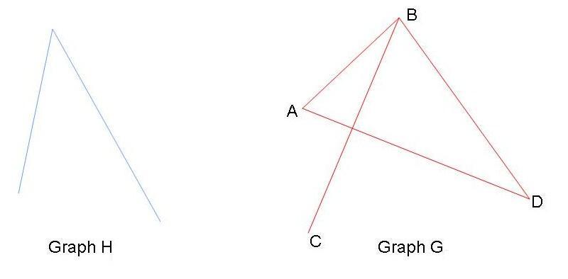
Figure 1: Constructing a lattice gas representation for the graph homomorphism density $t(H,G)$.

The above construction might be better explained with a concrete example. Take $H$ a two-star (with $m=3$ vertices and $p=2$ edges). Let $G$ (see Figure 1) be a finite simple graph on $4$ vertices ($n=4$): $A$, $B$, $C$, and $D$. There are $18$ homomorphisms and $4^{3}=64$ total mappings from $V(H)$ to $V(G)$. By (1), the homomorphism density of $H$ in $G$ is $t(H,G)=18/64$.

The density $t(H,G)$ may be derived through a lattice gas representation as well. For notational convenience, we denote $d(H,X)$ by $J(X)$. The image of $H$ in $G$ under a homomorphic mapping is either an edge or a two-star. The exact homomorphism density for an edge is $2/64$, and we have $J(\{A,B\})=J(\{A,C\})=J(\{A,D\})=J(\{B,C\})=J(\{B,D\})=J(\{C,D\})=2/64$. The exact homomorphism density for a two-star is also $2/64$, and we have $J(\{A,B\},\{B,C\})=J(\{B,A\},\{A,C\})=J(\{A,C\},\{C,B\})=J(\{A,B\},\{B,D\})=J(\{B,A\},\{A,D\})=J(\{A,D\},\{D,B\})=J(\{A,C\},\{C,D\})=J(\{C,A\},\{A,D\})=J(\{A,D\},\{D,C\})=J(\{B,C\},\{C,D\})=J(\{C,B\},\{B,D\})=J(\{B,D\},\{D,C\})=2/64$. For all other $X\subseteq E_{4}$, we have $J(X)=0$. The indicator function $\sigma$ of this particular $E(G)$ is given by: $\sigma_{\{A,B\}}=\sigma_{\{A,D\}}=\sigma_{\{B,C\}}=\sigma_{\{B,D\}}=1$ and $\sigma_{\{A,C\}}=\sigma_{\{C,D\}}=0$. Therefore the valid images of $H$ in $G$ are: edges $AB$, $AD$, $BC$, $BD$, each carrying density $2/64$; two-stars $(AB,BC)$, $(AB,BD)$, $(CB,BD)$, $(BA,AD)$, $(AD,DB)$, each carrying density $2/64$, making the combined density $\sum_{X\subseteq E_{4}}J(X)\sigma_{X}=18/64$.

As $n$ gets large, it would seem hard to keep track of all the densities $d(H,X)$ in the lattice gas representation, nevertheless, we will show that the pinned densities have a universal upper bound.

Proposition 2.4.

Let $G\in\mathcal{G}_{n}$. Fix a finite simple graph $H$ with $m$ vertices. Fix a vertex pair $e=\{i,j\}$ of $G$. Denote by $t_{e}(H,G)$ the sum of the exact homomorphism densities $d(H,X)$ with $e\in X\subseteq E(G)$. Then in the lattice gas representation (cf. Proposition 2.3), we have

$$t_{e}(H,G)=\sum_{X:e\in X\subseteq E(G)}d(H,X)\leq\frac{m(m-1)}{n^{2}}.$$ (8)

Proof.

The homomorphisms under consideration must satisfy that the image of $V(H)$ in $V(G)$ contain vertices $i$ and $j$ of $G$. To count these homomorphisms, we regard such a mapping as consisting of two steps. Step $1$: We construct vertex maps from $V(H)$ to $V(G)$: First select two vertices of $H$ to map onto $i$ and $j$, of which there are $m(m-1)$ choices. Then map the remaining vertices of $H$ onto $G$, of which there are $n^{m-2}$ ways. Step $2$: We check whether these vertex maps are valid homomorphisms (i.e. edge-preserving). The number of homomorphisms is thus bounded by $m(m-1)n^{m-2}$. Our claim easily follows once we recall that the total number of mappings from $V(H)$ to $V(G)$ is $n^{m}$. ∎

Our next theorem formulates the exponential random graph model as a lattice gas model. The lattice is $E_{n}$, the set of all vertex pairs $e$ of $V_{n}$. For each site $e=\{i,j\}$, we attach a lattice gas variable $\sigma_{e}$ which takes on the value $1$ or $0$. This specifies a simple graph $G$ on $V_{n}$ by Definition 2.1. The Hamiltonian $H(\sigma)$ is a weighted sum of graph homomorphism densities $t(H_{i},G)$ and varies according to the structure of the graph $G$ (cf. Proposition 2.3). It has a finite Banach space norm which depends on the universal upper bound for the pinned densities $d(H_{i},X)$ (cf. Proposition 2.4). This model is somewhat unconventional in the sense that the underlying lattice is “infinite-dimensional” (a vertex pair $e_{1}$ is a nearest neighbor of another vertex pair $e_{2}$ as long as they have a vertex in common, so the number of nearest neighbors of a given site grows with $n$, rather than being fixed at $2^{d}$ in a $d$-dimensional lattice), yet the associated interaction is finite-body. A key interest in this model is its behavior in the large $n$ limit. For that purpose, we will pay special attention to the limiting free energy as it is the generating function for the expectations of other random variables.

Theorem 2.5.

The general exponential random graph model (3) is equivalent to a lattice gas model with a finite Banach space norm.

Proof.

The Hamiltonian is the negative of the exponent of the probability mass function (3) (without normalization):

$$H(\sigma)=-n^{2}\sum_{i=1}^{k}\beta_{i}t(H_{i},G),$$ (9)

where $\sigma$ is the indicator function of $E(G)$. By Proposition 2.3, it has a lattice gas representation

$$H(\sigma)=-n^{2}\sum_{i=1}^{k}\beta_{i}\sum_{X\subseteq E_{n}}d(H_{i},X)\sigma_{X}.$$ (10)

Let $K(X)$ be the weighted sum of exact homomorphism densities $d(H_{i},X)$:

$$K(X)=n^{2}\sum_{i=1}^{k}\beta_{i}d(H_{i},X).$$ (11)

The Hamiltonian notation may then be simplified,

$$H(\sigma)=-\sum_{X\subseteq E_{n}}K(X)\sigma_{X}.$$ (12)

The interactions $K=\{K(X):X\subseteq E_{n}\}$ vary with the tuning parameters $\beta_{i}$ and form a Banach space $\mathcal{B}$. Define the $\mathcal{B}$-norm of $K$ by

$$||K||=\sup_{e}\sum_{X:e\in X}|K(X)|.$$ (13)

By Proposition 2.4,

$$||K||\leq m(m-1)\sum_{i=1}^{k}|\beta_{i}|.$$ (14)

This Banach space construction will be useful later on. ∎

Notice that $K(X)$, being a weighted sum of $d(H_{i},X)$, satisfies the finite-body property: $K(X)=0$ for $|X|>p$ (its importance to be illustrated in the proof of Lemma 3.6). Moreover, summing over $G\in\mathcal{G}_{n}$ (4) is equivalent to summing over indicator functions $\sigma$ of $E(G)\subseteq E_{n}$:

$$\sum_{G\in\mathcal{G}_{n}}\exp\left(n^{2}\sum_{i=1}^{k}\beta_{i}t(H_{i},G)\right)=\sum_{\sigma}\exp\left(-H(\sigma)\right).$$ (15)

Define $\psi^{\beta}$ to be the limiting free energy of the random graph model, i.e., $\psi^{\beta}=\lim_{n\rightarrow\infty}\psi^{\beta}_{n}$. By (4), (12), and (15), we have

$$\psi^{\beta}=\lim_{n\rightarrow\infty}\frac{1}{n^{2}}\log\left(\sum_{\sigma}\exp\left(\sum_{X\subseteq E_{n}}K(X)\sigma_{X}\right)\right).$$ (16)

We normalize the sum over $\sigma$ for the ease of cluster expansion. Henceforth $\sum^{\text{norm}}_{\sigma}$ will denote the normalized sum and satisfy $\sum^{\text{norm}}_{\sigma}1=1$, i.e., $\sum^{\text{norm}}_{\sigma}=2^{-|E_{n}|}\sum_{\sigma}=2^{-{n\choose 2}}\sum_{\sigma}$. Define the partition function $W$ by

$$W=\sum^{\text{norm}}_{\sigma}\exp\left(-H(\sigma)\right)=\sum^{\text{norm}}_{\sigma}\exp\left(\sum_{X\subseteq E_{n}}K(X)\sigma_{X}\right).$$ (17)

According to standard statistical mechanics, the limiting free energy $\phi^{\beta}$ of the lattice gas model is then given by

$$\phi^{\beta}=\lim_{n\rightarrow\infty}\frac{1}{|E_{n}|}\log W.$$ (18)

We explore the relationship between the two limiting free energies $\psi^{\beta}$ and $\phi^{\beta}$:

$$\psi^{\beta} = \lim_{n\rightarrow\infty}\frac{1}{n^{2}}\log\left(2^{n\choose 2}W\right)=\frac{1}{2}\left(\log 2+\lim_{n\rightarrow\infty}\frac{1}{{n\choose 2}}\log W\right)$$ (19)

$$= \frac{1}{2}\left(\log 2+\lim_{n\rightarrow\infty}\frac{1}{|E_{n}|}\log W\right)=\frac{1}{2}(\log 2+\phi^{\beta}).$$ (20)

The two interpretations of the limiting free energy are thus not appreciably different, and we may interpret it in either way to help with the understanding of the structure and behavior of the limiting network.

3 Cluster expansion

In this section we will apply cluster expansion techniques to derive a convergent power series expansion (high-temperature expansion) for the limiting free energy in the case of small parameters. The cluster expansion expressions presented here are completely rigorous for finite models, and may be interpreted in some more sophisticated limiting sense. We begin by introducing some combinatorial concepts. A hypergraph is a set of sites together with a collection $\Gamma$ of nonempty subsets. Such a nonempty set is referred to as a hyper-edge or link. Two links are connected if they overlap. The support of a hypergraph is the set $\cup\Gamma$ of sites that belong to some set in $\Gamma$. A hypergraph $\Gamma$ is connected if the support of $\Gamma$ is nonempty and cannot be partitioned into nonempty sets with no connected links. We use $\Gamma_{c}$ to indicate connectivity of the hypergraph $\Gamma_{c}$. Our first proposition gives a cluster representation for the partition function of the exponential random graph model.

Proposition 3.1.

Let $W$ be the partition function of the exponential random graph model on $n$ vertices (17). Then $W$ has a formal cluster representation

$$W=\sum_{\Delta}\prod_{N\in\Delta}w_{N},$$ (21)

where:

• $\Delta$ is a set of disjoint subsets $N$ of $E_{n}$.

• $w_{N}=\sum_{\cup\Gamma_{c}=N}\sum^{\text{norm}}_{\sigma|N}\prod_{X\in\Gamma_{c}}(\rme^{K(X)\sigma_{X}}-1).$

Proof.

We rewrite $\exp\left(\sum_{X\subseteq E_{n}}K(X)\sigma_{X}\right)$ as a perturbation around zero interaction,

$$W=\sum^{\text{norm}}_{\sigma}\prod_{X\subseteq E_{n}}\left(1+\rme^{K(X)\sigma_{X}}-1\right)=\sum^{\text{norm}}_{\sigma}\sum_{\Gamma}\prod_{X\in\Gamma}\left(\rme^{K(X)\sigma_{X}}-1\right),$$ (22)

where $\Gamma$ is a set of subsets $X$ of $E_{n}$.

We are going to organize the sum over hypergraphs in (22) in the following way. Let $N$ be a possible support for a connected hypergraph. Let $\Delta$ be a disjoint set of such sets $N$. Let $S$ be a function that takes $N\in\Delta$ to a hypergraph with support $N$, i.e., $\cup S(N)=N$. Then summing over hypergraphs $\Gamma$ is equivalent to summing over $\Delta$ and functions $S$ with the appropriate property. Furthermore, the product over $N$ in $\Delta$ and the links in $S(N)$ is equivalent to the product over the corresponding $\Gamma$. We have

$$W=\sum^{\text{norm}}_{\sigma}\sum_{\Delta}\sum_{S}\prod_{N\in\Delta}\prod_{X\in S(N)}\left(\rme^{K(X)\sigma_{X}}-1\right).$$ (23)

By independence, the sum over $\sigma$ can be factored over $\Delta$. Denote by $\sum^{\text{norm}}_{\sigma|N}$ the normalized sum restricted to subset $N$, i.e., $\sum^{\text{norm}}_{\sigma|N}=2^{-|N|}\sum_{\sigma|N}$. Similarly, denote by $\sum^{\text{norm}}_{\sigma|e}$ the normalized sum restriced to vertex pair $e$. This gives

$$W=\sum_{\Delta}\left(\prod_{e\notin\cup\Delta}\sum^{\text{norm}}_{\sigma|e}1\right)\sum_{S}\prod_{N\in\Delta}\sum^{\text{norm}}_{\sigma|N}\prod_{X\in S(N)}\left(\rme^{K(X)\sigma_{X}}-1\right).$$ (24)

Because of the normalization, $\sum^{\text{norm}}_{\sigma|e}1=1$, (24) can be simplified,

$$W=\sum_{\Delta}\sum_{S}\prod_{N\in\Delta}\sum^{\text{norm}}_{\sigma|N}\prod_{X\in S(N)}\left(\rme^{K(X)\sigma_{X}}-1\right).$$ (25)

Rearranging the terms by the distributive law, we have

$$W=\sum_{\Delta}\prod_{N\in\Delta}\sum_{\cup\Gamma_{c}=N}\sum^{\text{norm}}_{\sigma|N}\prod_{X\in\Gamma_{c}}\left(\rme^{K(X)\sigma_{X}}-1\right).$$ (26)

Our claim follows once we recall the definition of $w_{N}$. ∎

Notice that (21) has a graphical representation:

$$W = \sum_{n=0}^{\infty}\frac{1}{n!}\sum_{N_{1},...,N_{n}}\prod_{\{i,j\}}\left(1-t(N_{i},N_{j})\right)w_{N_{1}}\cdots w_{N_{n}}$$ (27)

$$= \sum_{n=0}^{\infty}\frac{1}{n!}\sum_{N_{1},...,N_{n}}c\left(N_{1},...,N_{n}\right)w_{N_{1}}\cdots w_{N_{n}},$$ (28)

where

$$c\left(N_{1},...,N_{n}\right)=\sum_{R}\prod_{\{i,j\}\in R}\left(-t(N_{i},N_{j})\right),$$ (29)

$R$ is a graph with vertex set $\{1,...,n\}$, and

$$t(N_{i},N_{j})=\left\{\begin{array}[]{ll}1&\mbox{if $N_{i}$ and $N_{j}$ overlap};\\ 0&\mbox{otherwise}.\end{array}\right.$$ (32)

This alternate expression of the partition function $W$ facilitates the application of cluster expansion ideas, which roughly summarized, state that a sum over arbitrary graphs can be written as the exponential of a sum over connected graphs. Taking the logarithm of the partition function (28) thus replaces the sum over graphs by the sum over connected graphs. The log operation is physically significant in that the resulting connected function $\log W$ is proportional to the limiting free energy $\phi^{\beta}$ (18). A detailed explanation of this phenomenon may be found, for instance, in a survey article by Faris [28].

Proposition 3.2.

Let $W$ be the partition function of the exponential random graph model on $n$ vertices (28). Then the connected function $\log W$ is given by the cluster expansion

$$\log W=\sum_{n=1}^{\infty}\frac{1}{n!}\sum_{N_{1},...,N_{n}}C\left(N_{1},...,N_{n}\right)w_{N_{1}}\cdots w_{N_{n}},$$ (33)

where

$$C\left(N_{1},...,N_{n}\right)=\sum_{R_{c}}\prod_{\{i,j\}\in R_{c}}\left(-t(N_{i},N_{j})\right),$$ (34)

and $R_{c}$ is a connected graph with vertex set $\{1,...,n\}$.

Now that we have derived an explicit expression for the connected function $\log W$, we explore criteria that guarantee the convergence of this expansion. This provides information on the limiting free energy $\phi^{\beta}$ (18) and characterizes the structure and behavior of the limiting network. The celebrated theorem of Kotecký and Preiss says that if the interaction is sufficiently weak, then the cluster expansion for the pinned connected function converges.

Theorem 3.3 (Kotecký-Preiss [29]).

Consider arbitrary family of activities $v_{N}\geq 0$. Suppose there are finite $B_{N}\geq 0$ such that for all $N_{0}$,

$$\sum_{N}t(N,N_{0})v_{N}B_{N}\leq\log B_{N_{0}}.$$ (35)

Then the pinned connected function has a convergent power series expansion in the polydisc $|w_{N}|\leq v_{N}$:

$$\sum_{n=1}^{\infty}\frac{1}{n!}\sum_{N_{1},...,N_{n}:\exists iN_{i}=N}\left|C\left(N_{1},...,N_{n}\right)\right||w_{N_{1}}|\cdots|w_{N_{n}}|\leq v_{N}B_{N}.$$ (36)

Remark.

In application it is convenient to take $B_{N}=M^{|N|}$ with $M>1$. With this choice of $B_{N}$ the Kotecký-Preiss condition is equivalent to the condition that (35) holds for all one point sets $N_{0}=\{e\}$:

$$\sum_{N:e\in N}v_{N}M^{|N|}\leq\log M.$$ (37)

This reduced version of the Kotecký-Preiss condition will be used throughout the rest of this section.

At first sight, the Kotecký-Preiss condition (37) seems very abstract and difficult to verify. It is a weighted sum of activities $v_{N}$ pinned at the vertex pair $e$, and each $v_{N}$ is an upper bound for $|w_{N}|$, whose expression involves a hypergraph decomposition and is rather complicated by itself (cf. Proposition 3.1). The following proposition gives a handy criterion for weak interaction in the small parameter region ($\sum_{i=1}^{k}|\beta_{i}|$ small).

Proposition 3.4.

Fix $M>1$. Take $w_{N}$ as in Proposition 3.1. It is clear that

$$|w_{N}|\leq v_{N}=\sum_{\cup\Gamma_{c}=N}\prod_{X\in\Gamma_{c}}(\rme^{|K(X)|}-1).$$ (38)

Consider the interaction $K$ with the Banach space norm $||K||$ (cf. Theorem 2.5). Suppose $\sum_{i=1}^{k}|\beta_{i}|$ is small:

$$||K||\leq m(m-1)\sum_{i=1}^{k}|\beta_{i}|\leq\frac{\log M(p-1)^{p}}{2(Mp)^{p}\left(1+(p-1)\log M\right)}.$$ (39)

Then (37) holds for every vertex pair $e$.

Remark.

The maximal region of parameters $\{\beta_{i}\}$ is obtained by setting

$$\log M=\frac{-p+\sqrt{5p^{2}-4p}}{2p(p-1)}.$$ (40)

Our ultimate goal is to examine convergence of the limiting free energy $\phi^{\beta}$ (18), which is proportional to the connected function $\log W$ (33). As the Kotecký-Preiss result concerns convergence of the pinned connected function (36), it appears to be inapplicable. However, our next theorem shows that pinning is actually the central ingredient that ties these two seemingly unrelated issues together.

Theorem 3.5 (Main Theorem).

Fix $M>1$. Consider the interaction $K$ with the Banach space norm $||K||$ (cf. Theorem 2.5). Suppose $\sum_{i=1}^{k}|\beta_{i}|$ is small (39). Then the limiting free energy $\phi^{\beta}$ (18) is analytic in $\beta$ and the rate of convergence is uniform.

Proof.

By Proposition 3.4, (37) holds for every vertex pair $e$. The pinned connected function (36) thus converges absolutely by Theorem 3.3, which further implies

$$|\log W| \leq \sum_{N\subseteq E_{n}}\sum_{n=1}^{\infty}\frac{1}{n!}\sum_{N_{1},...,N_{n}:\exists iN_{i}=N}\left|C\left(N_{1},...,N_{n}\right)\right||w_{N_{1}}|\cdots|w_{N_{n}}|$$ (41)

$$\leq \sum_{N\subseteq E_{n}}v_{N}M^{|N|}\leq\sum_{e\in E_{n}}\sum_{N:e\in N}v_{N}M^{|N|}\leq|E_{n}|\log M.$$ (42)

We conclude that the limiting free energy $\phi^{\beta}$ is absolutely convergent and bounded above by $\log M$. ∎

The rest of this section is devoted to the proof of Proposition 3.4. The weighted activity sum in the Kotecký-Preiss weak interaction condition (37) is rewritten as a power series, whose terms are then shown to be exponentially small under (39) by a series of lemmas.

Proof of Proposition 3.4. We notice that when $||K||$ is small (say $||K||\leq\frac{1}{2}$), $\rme^{|K(X)|}-1\leq 2|K(X)|$ by the mean value theorem. For $\cup\Gamma_{c}=N$, $|N|\leq\sum|X|$ with $X$ in $\Gamma_{c}$. We have

$$\sum_{N:e\in N}v_{N}M^{|N|} \leq \sum_{N:e\in N}\sum_{\cup\Gamma_{c}=N}M^{|N|}\prod_{X\in\Gamma_{c}}2|K(X)|$$ (43)

$$\leq \sum_{\Gamma_{c}:e\in\cup\Gamma_{c}}\prod_{X\in\Gamma_{c}}2|K(X)|M^{|X|}.$$ (44)

We say that a hypergraph $\Gamma_{c}$ is rooted at the vertex pair $e$ if $e\in\cup\Gamma_{c}$. Let $a_{n}(e)$ be the contribution of all connected hypergraphs with $n$ links that are rooted at $e$,

$$a_{n}(e)=\sum_{e\in\cup\Gamma_{c}:|\Gamma_{c}|=n}\prod_{X\in\Gamma_{c}}2|K(X)|M^{|X|}.$$ (45)

Then

$$\sum_{N:e\in N}v_{N}M^{|N|}\leq\sum_{n=1}^{\infty}\sup_{e\in E_{n}}a_{n}(e):=\sum_{n=1}^{\infty}a_{n}.$$ (46)

It seems that once we show that $a_{n}$ is exponentially small, the power series above will converge, and our claim might follow. To estimate $a_{n}$, we relate to some standard combinatorial facts [30]. ∎

Lemma 3.6.

Let $a_{n}$ be the supremum over $e$ of the contribution of connected hypergraphs with $n$ links that are rooted at $e$. Then $a_{n}$ satisfies the recursive bound

$$a_{n}\leq 2||K||M^{p}\sum_{k=0}^{p}{p\choose k}\sum_{a_{n_{1}},...,a_{n_{k}}:n_{1}+...+n_{k}+1=n}a_{n_{1}}\cdots a_{n_{k}}$$ (47)

for $n\geq 1$, where ${p\choose k}$ is the binomial coefficient.

Proof.

We linearly order the vertex pairs $e$ in $E_{n}$ and also linearly order the subsets $X$ of $E_{n}$. For a fixed but arbitrarily chosen $e$ in $E_{n}$, we examine (45). Write $\Gamma_{c}=\{X_{1}\}\cup\Gamma^{1}_{c}$, where $X_{1}$ is the least $X$ in $\Gamma_{c}$ with $e\in X_{1}$. As $K(X_{1})\neq 0$ only for $|X_{1}|\leq p$,

$$a_{n}(e)\leq 2||K||M^{p}\sum_{\Gamma^{1}_{c}}\prod_{X\in\Gamma^{1}_{c}}2|K(X)|M^{|X|}.$$ (48)

The remaining hypergraph $\Gamma^{1}_{c}$ has $n-1$ subsets and breaks into $k:k\leq p$ connected components (which again follows from the finite-body property of $K$). Say they are $\Gamma_{1},...,\Gamma_{k}$ of sizes $n_{1},...,n_{k}$, with $n_{1}+...+n_{k}=n-1$. For each component $\Gamma_{i}$, there is a least vertex pair $e_{i}$ through which it is connected to $X_{1}$, i.e., $e_{i}\in X_{1}$ is a root of $\Gamma_{i}$. As $|X_{1}|\leq p$ and $\Gamma^{1}_{c}$ consists of $k$ components, the number of possible choices for the root locations is at most ${p\choose k}$. We have

$$a_{n}(e)\leq 2||K||M^{p}\sum_{k=0}^{p}{p\choose k}\sum_{a_{n_{1}},...,a_{n_{k}}:n_{1}+...+n_{k}+1=n}a_{n_{1}}\cdots a_{n_{k}}.$$ (49)

Our inductive claim follows by taking the supremum over all $e$ in $E_{n}$. Finally, we look at the base step: $n=1$. In this simple case, as reasoned above, we have

$$a_{1}=\sup_{e\in E_{n}}\sum_{e\in\cup\Gamma_{c}:|\Gamma_{c}|=1}\prod_{X\in\Gamma_{c}}2|K(X)|M^{|X|}\leq 2||K||M^{p},$$ (50)

and this verifies our claim. ∎

Clearly, $\sum_{N:e\in N}v_{N}M^{|N|}$ will be bounded above by $\sum_{n=1}^{\infty}\bar{a}_{n}$, if

$$\bar{a}_{n}=2||K||M^{p}\sum_{k=0}^{p}{p\choose k}\sum_{\bar{a}_{n_{1}},...,\bar{a}_{n_{k}}:n_{1}+...+n_{k}+1=n}\bar{a}_{n_{1}}\cdots\bar{a}_{n_{k}}$$ (51)

for $n\geq 1$, i.e., equality is obtained in the above lemma. Observe that when $n=1$, the empty product (corresponding to $k=0$) is the only nonzero term on the right side of (51), so we have $\bar{a}_{1}=2||K||M^{p}$, matching the bound in (50).

Lemma 3.7.

Consider the coefficients $\bar{a}_{n}$ that bound the contributions of connected and rooted hypergraphs with $n$ links. Let $w=\sum_{n=1}^{\infty}\bar{a}_{n}z^{n}$ be the generating function of these coefficients. The recursion relation (51) for the coefficients is equivalent to the formal power series generating function identity

$$w=2||K||M^{p}z(1+w)^{p}.$$ (52)

Proof.

Notice that $(1+w)^{p}=\sum_{k=0}^{p}{p\choose k}w^{k}$, thus

$$w=2||K||M^{p}z\sum_{k=0}^{p}{p\choose k}w^{k}.$$ (53)

Writing completely in terms of $z$, we have

$$\sum_{n=1}^{\infty}\bar{a}_{n}z^{n}=2||K||M^{p}\sum_{k=0}^{p}{p\choose k}\sum_{\bar{a}_{n_{1}},...,\bar{a}_{n_{k}}:n_{1}+...+n_{k}+1=n}\bar{a}_{n_{1}}\cdots\bar{a}_{n_{k}}z^{n}.$$ (54)

We compare the coefficient of $z$ on both sides of (54): On the left it is given by $\bar{a}_{1}$, and on the right it is given by $2||K||M^{p}$ times the empty product, thus $\bar{a}_{1}=2||K||M^{p}$. Our general claim follows from term-by-term comparison. ∎

Lemma 3.8.

If $w$ is given as a function of $z$ as a formal power series by the generating function identity (52), then this power series has a nonzero radius of convergence $|z|\leq\frac{(p-1)^{p-1}}{2||K||(Mp)^{p}}$.

Proof.

Without loss of generality, assume $z\geq 0$. Set $z_{1}=2||K||M^{p}z$. Solving (52) for $z_{1}$ gives $z_{1}=w/(1+w)^{p}$. As $z_{1}$ goes from $0$ to $(p-1)^{p-1}/{p^{p}}$, the $w$ values range from $0$ to $1/(p-1)$. ∎

Proof of Proposition 3.4 continued. We notice that in the above lemma, $w=\sum_{n=1}^{\infty}\bar{a}_{n}z^{n}=1/(p-1)$ corresponds to $2||K||M^{p}z=(p-1)^{p-1}/{p^{p}}$, which implies that for each $n$,

$$\bar{a}_{n}\leq\left(2||K||(Mp)^{p}\right)^{n}\left(p-1\right)^{-\left(1+(p-1)n\right)}.$$ (55)

Gathering all the information we have obtained so far,

$$\sum_{N:e\in N}v_{N}M^{|N|} \leq \sum_{n=1}^{\infty}\left(2||K||(Mp)^{p}\right)^{n}\left(p-1\right)^{-\left(1+(p-1)n\right)}$$ (56)

$$= \frac{\frac{2||K||(Mp)^{p}}{(p-1)^{p}}}{1-\frac{2||K||(Mp)^{p}}{(p-1)^{p-1}}}\leq\log M.$$ (57)

by (39). ∎

4 Concluding remarks

This paper reveals a deep connection between random graphs and lattice gas (Ising) systems, making the exponential random graph model treatable by cluster expansion techniques from statistical mechanics. We show that any exponential random graph model may alternatively be viewed as a lattice gas model with a finite Banach space norm and derive a convergent power series expansion (high-temperature expansion) for the limiting free energy in the case of small parameters. Since the free energy is the generating function for the expectations of other random variables, this characterizes the structure and behavior of the limiting network in this parameter region. We hope this rigorous expansion will provide insight into the limiting structure of exponential random graphs in other parameter regions and shed light on the application of renormalization group ideas to these models.

References

References

- [1] Fienberg S, Introduction to papers on the modeling and analysis of network data, 2010 Ann. Appl. Statist. 4 1
- [2] Fienberg S, Introduction to papers on the modeling and analysis of network data II, 2010 Ann. Appl. Statist. 4 533
- [3] Solomonoff R and Rapoport A, Connectivity of random nets, 1951 Bull. Math. Biophys. 13 107
- [4] Erdős P and Rényi A, On the evolution of random graphs, 1960 Publ. Math. Inst. Hung. Acad. Sci 5 17
- [5] Watts D and Strogatz S, Collective dynamics of ‘small-world’ networks, 1998 Nature 393 440
- [6] Strogatz S, Exploring complex networks, 2001 Nature 410 268
- [7] Dorogovtsev S and Mendes J, Evolution of Networks: From Biological Nets to the Internet and WWW, 2003 Oxford University Press, Oxford
- [8] Meyers L, Newman M, Martin M and Schrag S, Applying network theory to epidemics: Control measures for outbreaks of Mycoplasma pneumoniae, 2001 Emerging Infectious Diseases 9 204
- [9] Newman M, Watts D and Strogatz S, Random graph models of social networks, 2002 Proc. Natl. Acad. Sci. USA 99 2566
- [10] Holland P and Leinhardt S, An exponential family of probability distributions for directed graphs, 1981 J. Amer. Statist. Assoc. 76 33
- [11] Frank O and Strauss D, Markov graphs, 1986 J. Amer. Statist. Assoc. 81 832
- [12] Wasserman S and Faust K, Social Network Analysis: Methods and Applications, 2010 Structural Analysis in the Social Sciences, Cambridge University Press, Cambridge
- [13] Snijders T, Pattison P, Robins G and Handcock M, New specifications for exponential random graph models, 2006 Sociol. Method. 36 99
- [14] Rinaldo A, Fienberg S and Zhou Y, On the geometry of discrete exponential families with application to exponential random graph models, 2009 Electron. J. Stat. 3 446
- [15] Häggström O and Jonasson J, Phase transition in the random triangle model, 1999 J. Appl. Probab. 36 1101
- [16] Park J and Newman M, Solution of the two-star model of a network, 2004 Phys. Rev. E 70 066146
- [17] Park J and Newman M, Solution for the properties of a clustered network, 2005 Phys. Rev. E 72 026136
- [18] Borgs C, Chayes J, van der Hofstad R, Slade G and Spencer J, Random subgraphs of finite graphs: III. The phase transition for the -cube, 2006 Combinatorica 26 395
- [19] Bollobás B, Janson S and Riordan O, The phase transition in inhomogeneous random graphs, 2007 Random Structures Algorithms 31 3
- [20] Bhamidi S, Bresler G and Sly A, Mixing time of exponential random graphs, 2008 Ann. Appl. Probab. 21 2146
- [21] Dembo A and Montanari A, Gibbs measures and phase transitions on sparse random graphs, 2010 Braz. J. Probab. Stat. 24 137
- [22] Lovász L and Szegedy B, Limits of dense graph sequences, 2006 J. Combin. Theory Ser. B 96 933
- [23] Chatterjee S and Diaconis P, Estimating and understanding exponential random graph models, 2011 arXiv: 1102.2650v3
- [24] Radin C and Yin M, Phase transitions in exponential random graphs, 2011 arXiv: 1108.0649v2
- [25] Aristoff D and Radin C, Emergent structures in large networks, 2011 arXiv: 1110.1912v1
-
[26]
Yin M, Understanding exponential random graph models, 2012
http://www.ma.utexas.edu/users/myin/Talk.pdf - [27] Yin M, Renormalization group transformations near the critical point: Some rigorous results, 2011 J. Math. Phys. 52 113507
- [28] Faris W, Combinatorics and cluster expansions, 2010 Probab. Surv. 7 157
- [29] Kotecký R and Preiss D, Cluster expansion for abstract polymer models, 1986 Commun. Math. Phys. 103 491
- [30] Malyshev V and Minlos R, Gibbs Random Fields: Cluster Expansions, 1991 Kluwer Academic Publishers, Dordrecht