A UBV Photometric Survey of the Kepler Field

Abstract

We present the motivations for and methods we used to create a new ground-based photometric survey of the field targeted by the NASA Kepler Mission. The survey contains magnitudes for 4414002 sources in one or more of the $UBV$ filters, including 1862902 sources detected in all three filters. The typical completeness limit is $U\sim 18.7$, $B\sim 19.3$, and $V\sim 19.1$ magnitudes, but varies by location. The area covered is 191 square degrees and includes the areas on and between the 42 Kepler CCDs as well as additional areas around the perimeter of the Kepler field. The major significance of this survey is our addition of $U$ to the optical bandpass coverage available in the Kepler Input Catalog, which was primarily limited to the redder SDSS griz and D51 filters. The $U$ coverage reveals a sample of the hottest sources in the field, many of which are not currently targeted by Kepler, but may be objects of astrophysical interest.

1 Introduction

The NASA Kepler Mission uses a 0.95m aperture space telescope targeting $>165000$ targets in a 115 square degree field in order to produce long-term light curves with the primary mission of detecting and characterizing transiting exoplanets (Borucki et al., 2010). In addition to the exoplanetary mission, the high-precision, long-term light curves have proved invaluable for studying many other astrophysical phenomena (e.g., Balona et al., 2011; Barth et al., 2011; Basri et al., 2011; Chaplin et al., 2011; Kawaler et al., 2010). Some of these astrophysical studies use stars selected on the basis of properties other than those indicating suitability as transiting exoplanet targets.

We carried out our survey of the Kepler field in $UBV$ filters primarily to create a resource for selecting new Kepler targets, although the new bandpass coverage also provides information that can help characterize the existing target list. Previous to this survey, the only similarly deep, optical survey covering the entire Kepler field in optical bandpasses had been the effort to create the Kepler Input Catalog (hereafter KIC; Brown et al. (2011)) for mission planning and target selection. The KIC is mainly limited to the SDSS $griz$ filters and gravity-sensitive $D51$ bandpass near 515 nm. Our new survey in $UBV$ provides photometric information across the Balmer Jump, and should be especially helpful in selecting new blue targets like O and B stars, hot white dwarfs, hot subdwarfs, planetary nebula central stars, cataclysmic variables, and AGN. At the same time, the Kepler-INT Survey, a collaboration of the UVEX (Groot et al., 2009) and IPHAS (Drew et al., 2005) surveys, is surveying the Kepler field using $Ugri$ and H$\alpha$ filters (see Greiss et al., 2012).

In this paper we describe our new 191 square degree $UBV$ photometric survey of the Kepler field. In § 2 we describe our observations. In § 3 we describe the image reductions, our methods to find instrumental magnitudes for sources in each exposure (under conditions that were not always photometric), and how we tied those magnitudes to the same scale using existing photometry from the KIC. In § 4 we present some basic results from the survey describing the usefulness of a photometric catalog produced by this survey as a resource for selecting new Kepler targets. In § 5 we announce the public availability of the data.

2 Observations

We observed the Kepler field using the NOAO Mosaic-1.1 Wide Field Imager and the WIYN 0.9m telescope on Kitt Peak, Arizona over the course of 5 nights between UT 2011 June 23-27. The observing conditions were partial moon illumination with a mixture of photometric skies and light clouds. The seeing FWHM ranged from $1\farcs 3-3\farcs 4$ in $U$, $1\farcs 2-2\farcs 9$ in $B$, and $1\farcs 2-2\farcs 5$ in $V$ with median seeing values of $1\farcs 7$, $1\farcs 5$, and $1\farcs 5$ in $U$, $B$, and $V$ respectively. The Mosaic-1.1 Wide Field Imager employs a mosaic of 8 $2048\times 4096$ pixel, thinned, AR-coated e2v CCDs (see Sawyer et al., 2010). Each CCD is read out through 2 amplifiers that read out $1024\times 4096$ pixel subarrays. On the 0.9m telescope, the CCD mosaic is arranged in a $4\times 2$ (North-South by East-West) pattern and spans a $59\arcmin\times 59\arcmin$ field-of-view with approximately $35\arcsec$ wide gaps between the CCDs and a plate scale of $0\farcs 43$ pixel^-1. The controllers provide 18-bit resolution in counts with a well depth exceeding 200,000 electrons. Details of the Mosaic-1.1 imager can be found at the Kitt Peak National Observatory web site. We observed using Johnson/Harris filters (Kitt Peak serial numbers k1001, k1002, and k1003 for $U$, $B$, and $V$ respectively).

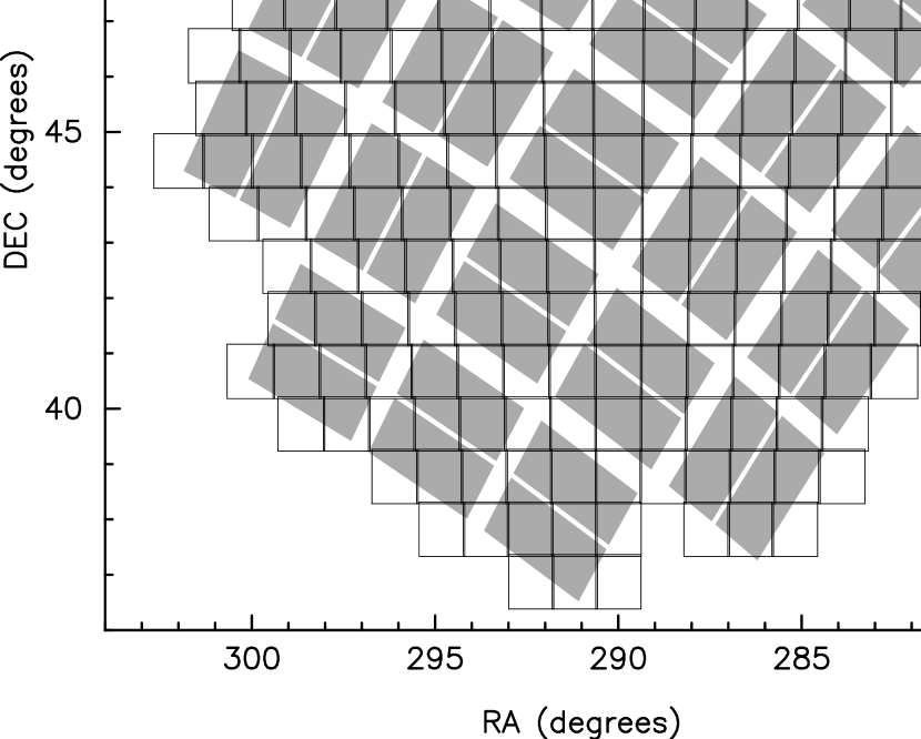
Figure 1: The grid of 206 slightly-overlapping $59\arcmin\times 59\arcmin$ pointings in our 191 square degree survey are shown as boxes overlaid on the grey regions representing the 42 Kepler CCDs.

We selected a set of 206 pointings that covered the Kepler field and surrounding areas in a grid pattern with $\sim 1$ arcmin overlaps between images at adjacent pointings. The position of our pointings and their relationship to the Kepler CCDs is shown in Figure 1. A few small areas at the edges of the Kepler field, the gaps between the Mosaic-1.1 CCDs, and a few areas masked out in our images account for the only areas within the survey region lacking photometry. These masks are defined to exclude bad or saturated pixels, cosmic rays, areas within halos surrounding the brightest stars, reflections in the optics that probably arise from stars lying just outside the images, and satellite trails. We estimate the total area covered at 191 square degrees.

At each pointing, we took consecutive exposures in $U$, $B$ and $V$ with exposure times of 180, 40, and 40 seconds respectively before moving to the next pointing. We observed some pointings (usually in all 3 filters) more than once after inspecting the quality of each image for poor seeing or lack of focus (the telescope focus drifted significantly during some exposures). Ultimately, only one exposure per filter per pointing is used in the survey. We tried whenever possible to use images that were taken in close succession (within $\sim 5$ minutes of one another). Our observations span an airmass range of $1.0-1.6$.

We obtained bias frames and dome flats each night for data calibration purposes.

3 Data Reduction

3.1 Pipeline Image Processing

Our image reduction methods start with a NOAO-based reduction pipeline that was developed for the Mosaic Camera and the Mayall 4-m Telescope (Swaters & Valdes, 2007; Valdes & Swaters, 2007). The 618 images (206 pointings with exposures in 3 filters at each) are input to the pipeline along with bias and dome flat data. The pipeline subtracts an overscan bias level from each image and a residual bias pattern for each CCD based on bias frames taken during the observing run. It then flatfields each image using the dome flats. Because the dome flat field screen is not ideal, the flattened images at this point have residual, large-scale non-flatness patterns. To correct these, the pipeline constructs a master sky flat using all dome flat corrected on-sky images taken during the run with deviant pixels (e.g., stars) filtered out. The sky flat is then applied to each image. The resulting product, known as “InstCal” images, is the basis of our survey photometry.

Unfortunately, there appeared to be a time-variable component in the 2-D bias pattern that manifested itself as changes to a low spatial frequency “bounce” or “ringing” pattern in the bias level across the beginning of each row next to the output amplifiers. Since this pattern wasn’t successfully subtracted from each individual image, it remained in the dome flat corrected images. From there, the same pattern emerged in the sky flat fields, where, if not removed, would have imposed an artificial pattern on fluxes along the edges of each CCD. In order to correct this problem, we chose to correct the sky flats by fitting a single 1-D function to the average of all rows of the flats in each readout region. We fitted the flux of the flats, $f$, for each readout region separately, parameterized using the coefficients $a_{1}...a_{6}$:

$$f(x)=a_{1}sin\left(\frac{x-a_{2}}{a_{3}}\right)\left(\frac{2}{2+e^{x/a_{4}}+e^{-x/a_{4}}}\right)+a_{5}+a_{6}x$$ (1)

Here, $x$ is the column number of each readout region as measured from the side with the amplifier. This function has a form that is a damped sine wave tilted to follow a line of constant slope. A correction to each sky flat is made by creating an image with values along each row of the readout regions given by $f(x)/(a_{5}+a_{6}x)$. We corrected the sky flats by dividing them by these corrections. Photometry of stars that are found on multiple overlapping images confirms the success of this procedure.

The pipeline reduction also detects saturated pixels, cosmic rays, CCD crosstalk features, and maps known bad pixels to create a bad pixel mask for each image. In addition, we manually inspected images for artifacts such as halos surrounding the brightest stars, reflections, and satellite trails. We added these features to the bad pixel masks to exclude the affected stars from our photometry.

Our astrometric plate solutions are also taken from the NOAO pipeline. To find plate solutions, the pipeline locates USNO-B1.0 Catalog stars (Monet et al., 2003) in each image. From the plate solution, we find coordinates for the photocenter of each source.

3.2 DAOPHOT Photometry

Our first step toward getting photometry of all the sources in our images is based on a recent version of DAOPHOT (Stetson, 1987) that is run separately on the exposure of each CCD. Our use of DAOPHOT consists of usual methods, and a minimum number of iterative steps which seem to be sufficient at the stellar densities encountered. The first step in the process is to find objects in each image using the “find” routine. Find detects the locations of flux peaks above a certain threshold relative to the expected noise on each CCD. The detection threshold can be varied, as can the allowable bounds on the “sharp” and “round” criteria describing the shapes of objects at each peak. We selected detection parameters in an attempt to maximize the detection of real sources and to minimize false detections. This method is fairly reliable in finding point sources and some galaxies with bright centers, but tends to avoid detecting galaxies with more diffuse light. Following object detection, we run the aperture photometry routine on each object, recording instrumental magnitudes in a series of concentric circular apertures around each star. In this case, the sky flux is estimated and subtracted based on measurements in an annulus centered on the stars and ranging between radii of $8\farcs 6$ and $15\farcs 1$. One aperture, with a radius of $1\farcs 3$, forms an initial estimate for the flux of each star.

We start DAOPHOT PSF-fitting photometry by picking a set of 40 optimal stars in each CCD that appear relatively bright and uncrowded. We use the “psf” routine to construct a single PSF model based on fitting a Penny model (Penny & Dickens, 1986) to the 40 stars. The PSF combines elliptical Gaussian and Lorentz functions in which the Gaussian component is rotated at an arbitrary angle but the Lorentz function is constrained to be elongated only along the array axes. Once the Penny model parameters are fitted to match the selected stars, the remaining component necessary to define the PSF is stored as a grid of look-up values. The resulting PSF can be scaled appropriately in flux and subtracted to “remove” stars from the image. We do this to remove stars close to our set of 40 PSF modelling stars and repeat our model fit to improve the PSF. After this step, we adopt the PSF model as our final solution and run the “allstar” routine to perform PSF-fitting photometry on every star in the image. In allstar, we fit the PSF model to each star out to a radius of $2\farcs 75$ and simultaneously estimate the sky level at each star based on a concentric annulus with inner and outer radii of $1\farcs 3$ and $8\farcs 6$.

The final steps that we apply to the lists of instrumental magnitudes for each exposure are aimed at removing stars that are false detections of background noise or artifacts like diffraction spikes from stars. Since the PSF-fitting process produces various outputs that correlate with false detections, we require that any sources remaining in the photometry lists require no more than a maximum number of iterations to be fit, that the $\chi^{2}_{\nu}$ of the PSF fits not be too large, and that the “sharp” shape parameter not be too high (as it would be for single-pixel features that are narrower than the characteristic PSF of the image). Lastly, even after applying our automatic methods to remove false detections, we found 73 CCD images that contained an anomalously high number of faint detections that could not be confirmed as valid objects upon visual inspection. These images are affected by unusually noisy readout patterns, and the false detections were identified in these patterns. For these images, we determined (by trial) a strict instrumental magnitude cut-off and we removed all detections fainter than these limits.

Once we had a final list of magnitudes, we cross-matched (by pixel coordinates) the data taken in each filter for each CCD of each pointing using the “daomatch” and “daomaster” programs, producing a single set of stars for each pointing (see the algorithm of Groth, 1986). We applied our plate solutions to define a single set of positions for each star. Since adjacent pointings overlap, we also have some stars that are common to between 2 and 4 neighboring pointings. We associate all of the photometry of these stars by cross-matching the data by their celestial coordinates. The cross-matched sources are all found by searching within a radius of $1\farcs 0$ to allow for some error in the plate solutions in field corners, although the mean separation between matched sources was $0\farcs 1$.

3.3 Photometric Calibration

The process of transforming our instrumental magnitudes measured in each image to either a common magnitude scale or an established photometric system is a complex task. It is made more difficult due to our desire to deliver this catalog to the public in a timely manner, the considerable area of the survey, the occasional non-photometric weather, and detailed calibration issues we would likely encounter in transforming photometry obtained with the Mosaic-1.1 Imager and Kitt Peak filters to photometric systems established using different instruments. Fortunately, optical photometry in the Kepler field already exists with the KIC and we were able to use stars common to both our data and the KIC to tie the magnitudes in our survey to a common scale. This is the most practical method to accomplish our primary objective of obtaining a sample of hot, $U$-band enhanced sources for use as future Kepler targets.

To correct our instrumental magnitudes to this common scale, we compared the photometry obtained on each of our CCDs separately to matching stars in the KIC, and to the same sources we observed on adjacent, overlapping pointings. We found a need to correct our instrumental magnitudes using three correction factors:

$$m(f,p,c)=m_{instr}(f,p,c)+C_{1}(f,p)+C_{2}(f,c)+C_{3}(f,p)$$ (2)

Here, $m$ is the corrected magnitude we wish to obtain, $m_{instr}$ is the instrumental magnitude we get from DAOPHOT as described in § 3.2, and $C_{1}$, $C_{2}$, and $C_{3}$ are separate magnitude corrections that have distinct values that depend variously on $f$, the filter used, $p$, the pointing observed, and $c$, the CCD on which a star is found. Although $C_{1}$ and $C_{3}$ have the same dependencies, we calculate them separately.

Our first step in correcting instrumental magnitudes was to apply a single offset, $C_{1}$, to the magnitudes measured in each exposure. This correction simultaneously corrects for a number of effects including first order atmospheric extinction, cloud extinction, and exposure-to-exposure differences in an aperture correction.

To find $C_{1}$, we selected a sample of 33610 calibrator stars from the KIC that are classified with $5500<T_{\rm eff}<6000$ K, log(gravity)$>4.2$, and have $g<15$ magnitudes. These stars were chosen because they are bright, fall among a relatively narrow range of colors, would be relatively unreddened, and are common in both surveys. We detected an average of 158 of these stars in each exposure. For each of these stars, we predicted a $B$ magnitude using the transformation from Jester et al. (2005):

$$B=g+0.39(g-r)+0.21$$ (3)

To predict $U$ and $V$ magnitudes for the same stars, we took the empirical broadband colors from Schmidt-Kaler (1982) for G5 dwarfs ($U-B=0.20$; $B-V=0.68$) and G0 dwarfs ($U-B=0.06$; $B-V=0.58$) to represent the predicted colors of stars with $T_{\rm eff}$ of 5500 K and 6000 K respectively. We predicted the colors of our calibrator stars by linearly interpolating the colors in this range based on values of $T_{\rm eff}$ in the KIC. Initial values for $C_{1}$ for each exposure could then be calculated as the median of the differences between our instrumental and the predicted magnitudes (with $C_{2}$ and $C_{3}$ momentarily set to zero).

The success of this procedure can be gauged by how well the magnitudes agree for stars that are detected more than once in a given filter. After our initial correction using $C_{1}$, the mean differences in magnitudes between overlapping pointings were generally low (the mean was 0.01 with standard deviation 0.02 magnitudes), but the range was $-0.15$ to 0.09 magnitudes. Additionally, we found some offsets of $\sim 0.05$ magnitudes when we considered the mean differences in magnitudes for individual pairs of overlapping CCDs. Thus, we deemed an additional correction $C_{2}$ to be necessary. To find $C_{2}$, we repeated the method we used to find $C_{1}$, but this time on a CCD-by-CCD rather than exposure-by-exposure basis. For each CCD, the different values of $C_{2}$ calculated for each exposure showed more scatter than did $C_{1}$, probably due to the smaller number of comparison stars available in each CCD. However, there was a similar pattern in each exposure, so we defined a set of 24 initial $C_{2}$ values (for the 8 CCDs and 3 filters) to be the median of the remaining corrections needed on each CCD after $C_{1}$ had been applied. The range of $C_{2}$ values (comparing the most disparate CCDs) spanned 0.090 magnitudes in $U$, 0.082 magnitudes in $B$ and 0.048 magnitudes in $V$.

Once we had initial values for both $C_{1}$ and $C_{2}$, we repeated the process once to recalculate a final set of $C_{1}$ values with our initial $C_{2}$ corrections applied. We then recalculated final values for $C_{2}$ with the final $C_{1}$ values applied. At this point, some of our exposures, which were scattered across the survey area, still showed magnitude offsets relative to neighboring pointings (as seen by systematic offsets in the magnitudes in overlapping image edges). The reason for these problematic exposures is unknown, but because $\sim 50$% or more of the adjacent exposures showed good agreement with one another, they can be used to anchor the magnitude scale across the field in each filter. We found a final set of corrections, $C_{3}$, to apply to 110 out of 206 $U$-band exposures, 91 out of 206 $B$-band exposures, and 65 out of 206 $V$-band exposures that reduces the remaining differences in magnitude measured in adjacent pointings. The values of $C_{3}$ were defined as the minimum correction needed to bring the mean difference in magnitudes of the deviant exposures to within 0.02 magnitudes of the mean of their overlapping neighbors, or set to zero otherwise. Standard deviations among the non-zero values of $C_{3}$ were 0.019, 0.015, 0.012 magnitudes for $U$, $B$, and $V$ filters respectively, but absolute values of $C_{3}$ ranged as high as 0.061 magnitudes for one exposure.

Finally, we associate each magnitude with an uncertainty arising from both random noise characteristics and systematic errors. We define the magnitude uncertainties as the quadrature sum of an error assigned by DAOPHOT, that incorporates the effects of noise and errors associated with fitting the PSF and sky subtraction, and a mostly systematic error that we find from our multiple exposures of the same stars. To determine the latter error component, we compare the mean differences in magnitudes observed on different CCDs for pairs of overlapping pointings. We define this systematic error component to be equal to $1/\sqrt{2}$ times the standard deviations of the magnitude differences, or 0.020 magnitudes in $U$, 0.023 magnitudes in $B$, and 0.017 magnitudes in $V$.

4 Results

Our survey contains magnitudes for 4414002 sources in one or more of the $UBV$ filters, including 1862902 sources detected in all three filters. This completeness in all three filters is primarily limited by the $U$-band data, for which we have 1895173 detections. In $B$ we have 3089223 detections, and in $V$, our most complete bandpass, we find 4363394 sources. A few sources remain that are spurious detections of background noise or features like diffraction spikes from other stars. These false detections could be essentially eliminated from a sample of catalog entries by requiring detections in two or more filters.

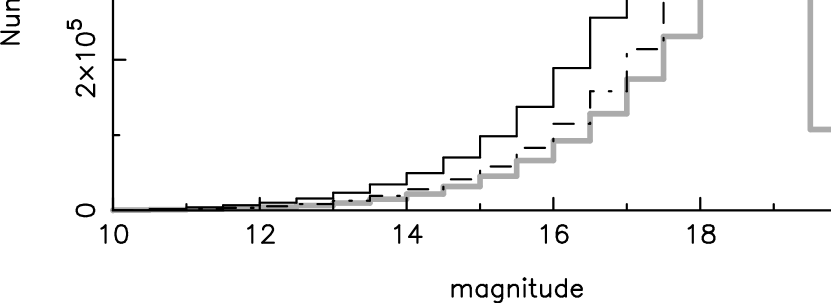
Figure 2: A histogram of the number of detected sources as functions of $U$, $B$, and $V$ magnitudes.

We plot the distribution of magnitudes in Fig. 2, which shows the wide dynamic range of the survey. The shape of the distribution is similar in each filter, but shifted toward slightly fainter magnitudes in $B$ and brighter magnitudes in $U$ when compared to $V$. While there is variation in our sensitivity from one pointing to another, we wished to estimate a rough, survey-wide completeness limit, the faint end of our magnitude range within which we expect to find almost all point sources in the field that lie on our detectors. To do this, we note that a logarithmically-scaled plot of number of sources vs. magnitude increases steadily with magnitude until some appreciable fraction of sources ($\sim 2$%) remain undetected in some exposures (probably due to relatively poor seeing). The overall survey appears complete to magnitudes $U\sim 18.7$, $B\sim 19.3$ and $V\sim 19.1$. Of course there are fainter sources in the survey (to about 1 magnitude fainter). The bright limits in our exposures are sensitive to the observing conditions, in particular the seeing. We estimate the bright limit, and its variation with location in our survey from the mean and standard deviations of the magnitudes of the brightest star in each exposure. For $U$ we find the mean and standard deviation to be 10.12 and 0.34, for $B$ it is 10.60 and 0.33, and for $V$ it is 10.55 and 0.30.

In Fig. 3 we plot the distribution of our uncertainties in magnitude as a function of magnitude for each filter. The uncertainties in each filter show a quantized distribution at low values of error due to the limited precision quoted for our data. With increasing brightness, the errors trend toward multiple lower limits (two of a total of four in each filter are most easily seen). The highest of these lower limits corresponds to the systematic photometric uncertainties discussed in § 3.3. For sources measured multiple times in overlapping pointings, our uncertainty is lower, accounting for the secondary lower limits. In addition to the systematic error component, which was applied to calculate each magnitude error, there are also exposure-to-exposure or star-to-star differences in uncertainties that show up in the plot as a broader scatter around the general trend versus magnitude. These errors can depend on the varying PSF in each image and source crowding. There are also uncertainties in our colors that can be propagated from these magnitude uncertainties. Color uncertainties reach lower limits of 0.030 for $U-B$ and 0.029 for $B-V$ for sources measured once in each filter. Once again, the errors for bright sources are mostly limited by the systematic errors discussed in § 3.3.

At this point we wish make a comparison of our magnitudes to those in the Hipparcos Catalogue (ESA, 1997) because it is known to be a source of well-calibrated photometry and was calibrated to match a standard magnitude scale. Unfortunately, the Hipparcos Catalogue contains mostly sources brighter than those in our survey. Nevertheless, there are 19 sources in common to the two catalogs that are not listed in the Hipparcos Catalogue as being known or suspected variables according to the coarse variability or HvarType flags. In Fig. 4 we plot the differences in $B$ and $V$ magnitudes between our survey and Johnson magnitudes in the Hipparcos Catalogue as a function of their $B-V$ colors. While most of the $B-V$ colors plotted are Johnson colors from Hipparcos, we use our own $B-V$ for the two stars lacking Hipparcos $B$ magnitudes. There is one very discrepant datum of $B-B_{\rm Hip}=-1.036$ for HIP95024, but with $B_{\rm Hip}=12.91$, this star has a Hipparcos magnitude 0.87 magnitudes fainter than any of the other stars we are comparing. Magnitude errors increase rapidly toward the faint limits of Hipparcos (ESA, 1997), so we leave this datum out of our analysis. Other stars with Hipparcos magnitudes fainter than 11.5 are shown using open symbols, but are considered in our analysis.

A comparison of our magnitudes to Hipparcos Johnson magnitudes reveals that there is an offset in the two magnitude scales of $V-V_{\rm Hip}=-0.023$ with a standard deviation $\sigma_{\rm{\Delta}V}=0.114$ and $B-B_{\rm Hip}=-0.008$ with a standard deviation $\sigma_{\rm{\Delta}B}=0.100$. Thus, any differences between the $B$ and $V$ magnitude scales of the two surveys are small. The lack of a larger magnitude offset is perhaps surprising given the considerable differences in the photometric methods used.

In Fig. 5 we show a two-color diagram of sources in the entire survey. As expected, most sources lie along the loci of the Main Sequence and Giant Branch. To define a subsample of the bluest sources in the survey, we select sources defined to satisfy both of the following color conditions: $U-B<-0.3$ and $U-B<-0.971(B-V)-0.057$. This area of color space lies above the lines in Fig. 5 and contains 3092 sources. The location of different stellar sources within this color region depends on factors like effective temperature, reddening, and composition. In order to refine our sample to sources that are most likely to be useful as new Kepler target stars, we define rectangular regions for each Kepler CCD using coordinates provided by the mission for one quarter of Kepler data. We find a subset of 1929 Kepler field sources among our blue sample. A histogram showing the magnitude distribution of these sources is given in Fig. 6. While most of these sources are fainter than the sample used for the mission’s exoplanet search (ie. fainter than $V\sim 16$), they are sufficiently bright to allow high-precision Kepler light curves and are good targets for ground-based classification spectroscopy. We anticipate that the photometric catalog produced from our survey will serve as a rich source of such targets.

5 Data Availability

The product of this survey is a publicly-available data catalog available for downloading or use as part of a cross-matched, multi-catalog, searchable database at the Multimission Archive at the Space Telescope Science Institute (MAST). The catalog includes the data from this survey (positions, magnitudes and their uncertainties) along with the products of other cross-matched catalogs, including the KIC. A detailed description of the catalog contents may be found at the website. In addition to the catalog, an interactive tool is planned that will provide sections of our reduced images to users for inspection.

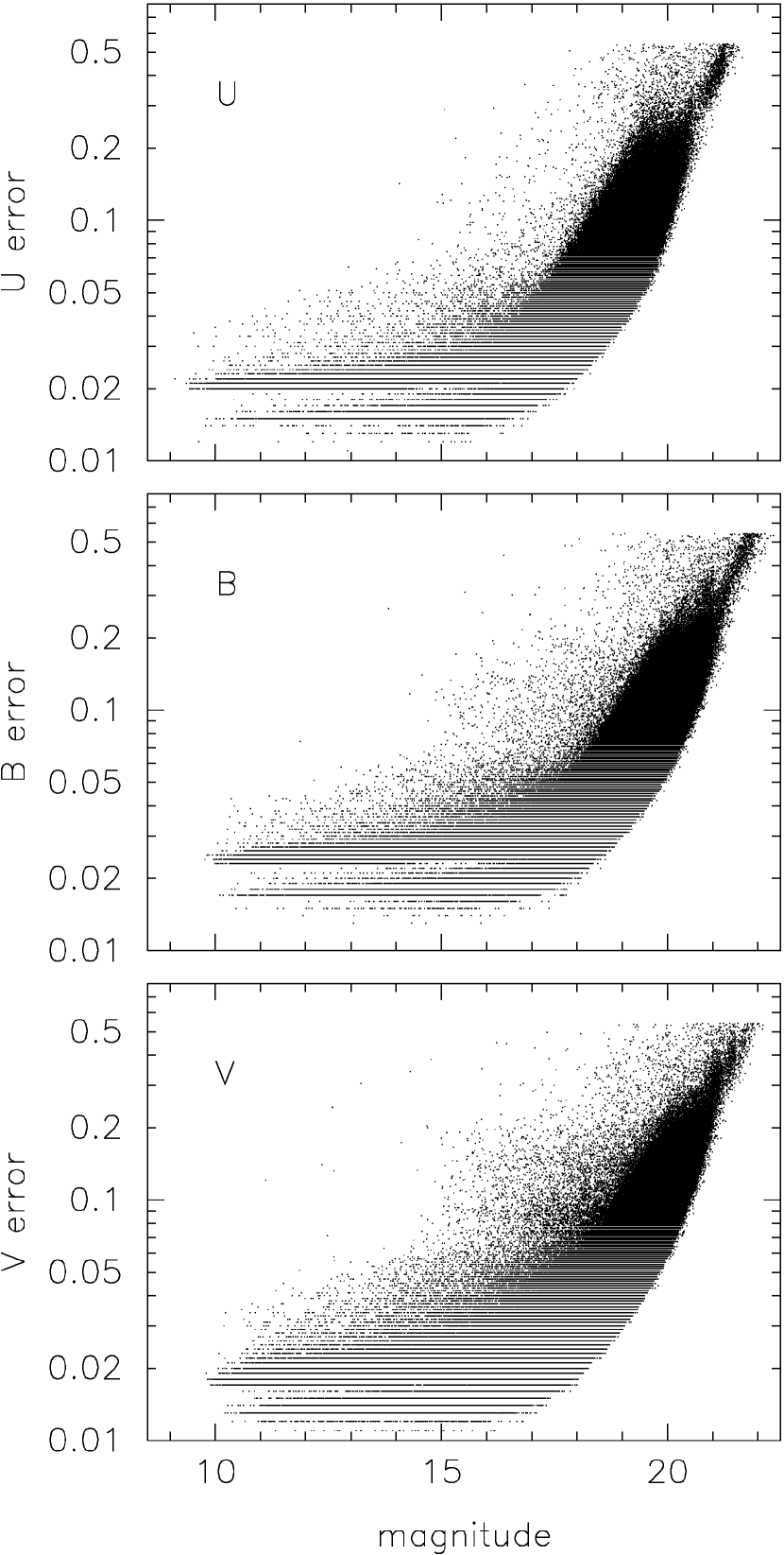
Figure 3: The uncertainties in each magnitude plotted as a function of magnitude in each filter. The distribution shows quantized values due to the limited precision quoted in our catalog. At bright magnitudes, the errors converge toward lower limits reflecting the systematic errors adopted for each filter. Because some sources are observed up to four times each, there are lower uncertainties for some measurements, giving rise to multiple sequences of points at low error values (see text for details).

Figure 4: A plot of the differences between our magnitudes and the corresponding Johnson magnitudes from the Hipparcos Catalogue as a function of the $B-V$ colors. The top panel shows a comparison of $V$ magnitudes while the bottom panel shows a comparison of $B$ magnitudes. The $B-V$ colors are taken from the Hipparcos Catalogue Johnson colors when available. The $B-V$ colors of two stars are taken from our survey. Stars having a Hipparcos Johnson magnitude fainter than 11.5 are shown as open circles.

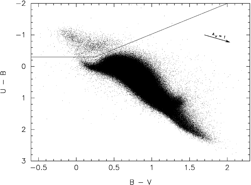
Figure 5: A two-color diagram of the 1.8 million sources detected in 3 filters showing the dominant Main Sequence and Giant Branch populations along with some outlier colors. The solid line segments define the upper limits in $U-B$ for a population of blue objects discussed in the text. Here the color region is defined to be $U-B<-0.3$ (shown in the horizontal line segment) and $U-B<-0.971(B-V)-0.057$ (the diagonal line segment).

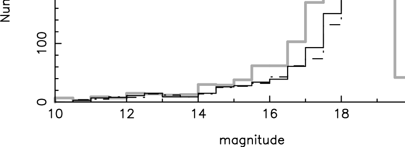
Figure 6: A histogram of the number of the bluest sources that lie in the Kepler field as functions of $U$, $B$, and $V$ magnitudes.

References

- Balona et al. (2011) Balona, L. A. et al. 2011, MNRAS, 413, 2403
- Barth et al. (2011) Barth, A. J. et al. 2011, ApJ, 732, 121
- Basri et al. (2011) Basri, G. et al. 2011, AJ, 141, 20
- Borucki et al. (2010) Borucki, W. J. et al. 2010, Science, 327, 977
- Brown et al. (2011) Brown, T. M., Latham, D. W., Everett, M. E., & Esquerdo, G. A. 2011, AJ, 142, 112
- Chaplin et al. (2011) Chaplin, W. J. et al. 2011, Science, 332, 213
- Drew et al. (2005) Drew, J. E. et al. 2005, MNRAS, 362, 753
- ESA (1997) ESA, 1997, The Hipparcos and Tycho Catalogues, ESA SP-1200
- Greiss et al. (2012) Greiss, S. et al. 2012, arXiv:1202.6333
- Groot et al. (2009) Groot, P. J. et al. 2009, MNRAS, 399, 323
- Groth (1986) Groth, E. J. 1986, AJ, 91, 1244
- Jester et al. (2005) Jester, S. et al. 2005, AJ, 130, 873
- Kawaler et al. (2010) Kawaler, S. D. et al. 2010, 409, 1509
- Monet et al. (2003) Monet, D. G. et al. 2003, AJ, 125, 984
- Penny & Dickens (1986) Penny, A. J., & Dickens, R. J. 1986, 220, 845
- Sawyer et al. (2010) Sawyer, D. G., Daly, P. N., Howell S. B., et al., 2010, SPIE, 7735, 111
- Schmidt-Kaler (1982) Schmidt-Kaler, T. 1982 in Landolt-Börnstein: Numerical Data and Functional Relationships in Science and Technology - New Series ”Group 6 Astronomy and Astrophysics” Volume 2 Schaifers/Voigt: Astronomy and Astrophysics Stars and Star Clusters, XV
- Stetson (1987) Stetson, P. B. 1987, PASP, 99, 191
- Swaters & Valdes (2007) Swaters, R. A. & Valdes, F. G. 2007, in ASP Conf. Ser. 376, Astronomical Data Analysis Software and Systems XVI, eds. R. A. Shaw, F. Hill, & D. J. Bell (San Francisco: ASP), 269
- Valdes & Swaters (2007) Valdes, F. G. & Swaters, R. A. 2007, in ASP Conf. Ser. 376, Astronomical Data Analysis Software and Systems XVI, eds. R. A. Shaw, F. Hill, & D. J. Bell (San Francisco: ASP), 273