Quantum Griffiths singularities in ferromagnetic metals

Abstract

We present a theory of the quantum Griffiths phases associated with the ferromagnetic quantum phase transition in disordered metals. For Ising spin symmetry, we study the dynamics of a single rare region within the variational instanton approach. For Heisenberg symmetry, the dynamics of the rare region is studied using a renormalization group approach. In both cases, the rare region dynamics is even slower than in the usual quantum Griffiths case because the order parameter conservation of an itinerant ferromagnet hampers the relaxation of large magnetic clusters. The resulting quantum Griffiths singularities in ferromagnetic metals are stronger than power laws. For example, the low-energy density of states $\rho(\epsilon)$ takes the asymptotic form $\exp[\{-\tilde{\lambda}\log(\epsilon_{0}/\epsilon)\}^{3/5}]/\epsilon$ with $\tilde{\lambda}$ being non-universal. We contrast these results with the antiferromagnetic case in which the systems show power-law quantum Griffiths singularities in the vicinity of the quantum critical point. We also compare our result with existing experimental data of ferromagnetic alloy ${\rm{Ni}}_{x}{\rm{V}}_{1-x}$.

I Introduction

The low-temperature behavior of quantum many-particle systems can be sensitive to impurities, defects, or other kinds of quenched disorder. This effect is especially important near quantum phase transitions, where fluctuations in time and space become connected. The interplay between static disorder fluctuations and large-scale quantum fluctuations leads to much more dramatic effects at quantum phase transitions than at classical phase transitions, including quantum Griffiths singularities, Griffiths (1969); Thill and Huse (1995); Rieger and Young (1996) infinite-randomness critical points featuring exponential rather than power-law scaling, Fisher (1992, 1995) and the smearing of the transition.Vojta (2003)

The Griffiths effects at a magnetic phase transition in a disordered system are caused by large spatial regions (rare regions) that are devoid of impurities and can show local magnetic order even if the bulk system is globally in the paramagnetic phase. The order parameter fluctuations induced by rare regions belong to a class of excitations known as instantons. Their dynamics is very slow because flipping the rare region requires a coherent change of the order parameter over a large volume. Griffiths showed Griffiths (1969) that this leads to a singular free energy, not just at the transition point but in a whole parameter region, which is now known as the Griffiths phase. In classical systems, the contribution of the rare regions to thermodynamic observables is very weak. However, due to the perfect disorder correlations in (imaginary) time, Griffiths effects at quantum phase transitions are enhanced and lead to power-law singularities in thermodynamic quantities (for reviews see, e.g., Refs. Vojta, 2006, 2010).

The systems in which quantum Griffiths behavior was originally demonstrated Thill and Huse (1995); Rieger and Young (1996); Fisher (1992, 1995) all have undamped dynamics (a dynamical exponent $z=1$ in the clean system). However, many systems of experimental importance involve superconducting Rogachev and Bezryadin (2003) or magnetic Löhneysen et al. (1994); Grigera et al. (2001); Pfleiderer et al. (1997); de Andrade et al. (1998) degrees of freedom coupled to conduction electrons. This leads to overdamped dynamics characterized by a clean dynamical exponent $z>1$. Studying the effects of the rare regions in this case is, therefore, an important issue. It has been shown that metallic Ising antiferromagnets can show quantum Griffiths behavior at higher energies, where the damping is less important. Castro Neto and Jones (2000) In contrast, the quantum Griffiths singularities in Heisenberg antiferromagnets are caused by the dissipation and occur at lower energies. Vojta and Schmalian (2005)

In recent years, indications of quantum Griffiths phases have been observed in experiments on a number of metallic systems suchs as magnetic semiconductors,Guo et al. (2008, 2010a, 2010b) Kondo lattice ferromagnets, Sereni et al. (2007); Westerkamp et al. (2009) and transition metal ferromagnets.Ubaid-Kassis et al. (2010); Schroeder et al. (2011) All these experimental observations of quantum Griffiths phases are in ferromagnets rather than in antiferromagnets. However, in contrast to antiferromagnets, a complete theory of quantum Griffiths phases in ferromagnetic metals does not yet exist.

In this paper, we therefore develop the theory of quantum Griffiths effects in ferromagnetic metals with both Ising and Heisenberg symmetries. We show that the quantum Griffiths singularities do not take power-law form, in contrast to those in antiferromagnets.Vojta (2006, 2010) The rare-region density of states behaves as $\rho(\epsilon)\sim\exp[\{-\tilde{\lambda}\log(\epsilon_{0}/\epsilon)\}^{3/5}]/\epsilon$ in the low-energy limit, where $\tilde{\lambda}$ plays a role analogous to the non-universal Griffiths exponent. This means that the Griffiths singularity is stronger than a pure power law. This kind of density of states leads to non-power-law dependencies on the temperature $T$ of various observables, including the specific heat, $C\!\sim\exp[\{-\tilde{\lambda}\log(T_{0}/T)\}^{3/5}]$, and the magnetic susceptibility, $\chi\!\sim\!\exp[\{-\tilde{\lambda}\log(T_{0}/T)\}^{3/5}]/T$. The zero-temperature magnetization-field curve behaves as $M\sim\exp[\{-\tilde{\lambda}\log(H_{0}/H)\}^{3/5}]$.

The paper is organized as follows. In Sec. II, we introduce the model: Landau-Ginzburg-Wilson order parameter field theories for ferromagnetic Ising and Heisenberg metals. In Sec. III, we study the dynamics of a single rare region. For the Ising case, we use a variational instanton calculation, and for Heisenberg symmetry, we use a renormalization group theory of the quantum nonlinear sigma model with a damping term. In Sec. IV, we average over all rare regions and calculate observables in the ferromagnetic quantum Griffiths phase. In Sec. V, we compare our predictions with existing experimental data. Finally, we conclude in Sec. VI by discussing the difference between ferromagnetic and antiferromagnetic quantum Griffiths singularities as well as some open questions.

II The model

Rare region effects in disordered metallic systems are realized both in Ising magnets Castro Neto and Jones (2000) and in Heisenberg magnets. Vojta and Schmalian (2005) In the following, we consider both cases. Our starting point is a quantum Landau-Ginzburg-Wilson action of the itinerant ferromagnet Hertz (1976); Millis (1993)^,

$$S=S_{\rm{stat}}+S_{\rm{diss}}+S_{\rm{dyn}}\,,$$ (1)

where the static part has the form

$$S_{\rm{stat}}= E_{0}\int_{0}^{\beta}d\tau\int d^{3}{\bf{r}}\Bigl{[}t\phi^{2}({\bf{r}},\tau)+[\nabla\phi({\bf{r}},\tau)]^{2}$$

$$+\frac{1}{2}\phi^{4}({\bf{r}},\tau)\Bigr{]}\,.$$ (2)

Here, $E_{0}$ is a characteristic energy (assumed to be of the order of the band width in a transition metal compound or the order of the Kondo-temperature in an $f$-electron system). We measure lengths in units of the microscopic length scale $\xi_{0}$. $t>0$ is the bare distance of the bulk system from criticality. $\phi({\bf{r}},\tau)$ is the dimensionless order parameter field. It is a scalar for the Ising model, while it has three components $(\phi_{1},\phi_{2},\phi_{3})$ for a Heisenberg magnet.

We consider disorder coupled to the square of the order parameter. The corresponding action has the form

$$S_{\rm{diss}}= E_{0}\int_{0}^{\beta}d\tau\int d^{3}{\bf{r}}\ V({\bf{r}})\phi^{2}({\bf{r}},\tau)\,,$$ (3)

where $V({\bf{r}})$ is the disorder potential.

The dynamical part of Eq. (1) is $S_{\rm{dyn}}=S^{(1)}_{\rm{dyn}}+S^{(2)}_{\rm{dyn}}$, where

$$S^{(1)}_{\rm{dyn}}=E_{0}\tau_{m}^{2}\int_{0}^{\beta}d\tau\int d^{3}{\bf{r}}[\partial_{\tau}\phi({\bf{r}},\tau)]^{2}\,,$$ (4)

corresponds to the undamped dynamics of the system with the clean dynamical exponent $z=1$, while

$$S^{(2)}_{\rm{dyn}}=\frac{\gamma T}{E_{0}}\sum_{\omega_{n}}|\omega_{n}|\int d^{3}\textbf{q}\ \frac{|\tilde{\phi}(\textbf{q},\omega_{n})|^{2}}{|\textbf{q}|^{a}}\,,$$ (5)

describes overdamped dynamics with conserved order parameter (clean dynamical exponent $z=2+a$), which stems from the coupling to the conduction electrons. In Eq. (4), $\tau_{m}$ is a microscopic time, and in Eq. (5), $\gamma$ parametrizes the strength of the dissipation. $\tilde{\phi}(\textbf{q},\omega_{n})$ is the Fourier transform of the order parameter $\phi({\bf{r}},\tau)$ in momentum and Matsubara frequency. The value of $a$ depends on the character of the electron motion in the system and equals 1 or 2 for ballistic and diffusive ferromagnets, respectively.

III Dynamics of a single rare region

In this section, we study the dynamics of a single droplet formed on a rare region of linear size $L$. This means, we consider a single spherical defect of radius $L$ at the origin with potential $V(r)=-V$ for $r<L$, and $V(r)=0$ otherwise. We are interested in the case $V>0$, i.e., in defects that favor the ordered phase.

The effective dimensionality of the model defined by Eq. (1) is $d_{\rm{eff}}=3+z.$ Thus, the clean model (1) is above its upper critical dimension ($d_{c}=4$), implying that mean-field theory is valid. The mean-field equation for a static order parameter configuration $\phi_{0}(r)$ is Millis et al. (2001)

$$\nabla^{2}\phi_{0}(r)+[t+V(r)]\phi_{0}(r)+\phi^{3}_{0}(r)=0\,,$$ (6)

with solution

$$\phi_{0}(r)=\left\{\begin{array}[]{lr}\hskip 5.69046pt\phi_{0}\hskip 38.12659pt\text{for}\hskip 14.22636ptr<L\\ \frac{\phi_{0}L}{r}e^{-rt^{1/2}}\hskip 8.5359pt\text{for}\hskip 14.22636ptr>L.\end{array}\right.$$ (7)

This implies that the order parameter is approximately constant in the region $r<L$ and decays outside of it.

To study the dynamics of the droplet, we start from the variational instanton approach.Millis et al. (2002) In the simplest case, the droplet maintains its shape while collapsing and reforming. In order to estimate the action associated with this process, we make the ansatz

$$\phi(r,\tau)=\phi^{\prime}_{0}(r)\eta(\tau)\,.$$ (8)

Here, $\phi^{\prime}_{0}(r)$ must be chosen such that $\int d^{3}{\bf{r}}\phi(r,\tau)$ is time independent because of order parameter conservation in an itinerant ferromagnet. This can be done by introducing $\phi^{\prime}_{0}(r)=\phi_{0}(r)(1-Ar)$ such that the $\textbf{q}=0$ Fourier component is canceled. $A$ is a constant to be determined. In the limit of a large rare region, $Lt>>1,$ we find

$$\phi^{\prime}_{0}(r)=\phi_{0}(r)\left(1-\frac{4}{3}\frac{r}{L}\right)\,.$$ (9)

In the following subsections, using ansatz Eq. (8), we separately discuss the dynamics of the droplet in itinerant Ising and Heisenberg ferromagnets.

III.1 Itinerant Ising model

We now calculate the tunneling rate between the “up” and “down” states of a single rare region in an itinerant Ising ferromagnet by carrying out variational instanton calculations.Millis et al. (2002); Hoyos and Vojta (2007) To estimate the instanton action, we use the ansatz Eq. (8) (which provides a variational upper bound for the instanton action) with $\eta(\tau)=\pm 1$ for $\tau\rightarrow\pm\infty$. Inserting this ansatz into the action Eq. (1) and integrating over the spatial variables yields, up to constant prefactors,

$$S_{\rm{stat}}\sim L^{3}\int d\tau[-2\eta^{2}(\tau)+\eta^{4}(\tau)]\,,$$ (10)

and

$$S^{(1)}_{\rm{dyn}}\sim L^{3}\int d\tau[\partial_{\tau}\eta(\tau)]^{2}\,.$$ (11)

The part of the action corresponding to the overdamped dynamics becomes

$$S^{(2)}_{\rm{dyn}}=\frac{\alpha}{4}\int d\tau d\tau^{\prime}\frac{d\eta}{d\tau}\frac{d\eta}{d\tau^{\prime}}\log\frac{(\tau-\tau^{\prime})^{2}+\tau^{2}_{m}}{\tau^{2}_{m}}\,,$$ (12)

where the dimensionless dissipation strength $\alpha\sim\gamma L^{3+a}$. In order to estimate the action Eqs. (10) to (12), we make the variational ansatz

$$\frac{d\eta}{d\tau}=\frac{2\theta(\tau^{2}_{0}-4\tau^{2})}{\tau_{0}}\,.$$ (13)

Summing all contributions, we obtain the instanton action

$$S\sim L^{3}/\tau_{0}+L^{3}\tau_{0}+\gamma L^{3+a}\log(\tau_{0}/\tau_{m})\,.$$ (14)

Minimizing this action over the instanton duration gives $\tau_{0}\sim L^{-a}/\gamma$. Correspondingly, the action is $S\sim\gamma L^{3+a}$. Then, the bare tunneling rate or tunnel splitting behaves as

$$\epsilon\sim\exp(-S)\sim\exp({-{\rm{const.}}\times\gamma L^{3+a}})\,.$$ (15)

Thus, the bare tunneling rate decays exponentially with $L^{3+a}$ in the itinerant Ising ferromagnet unlike the tunneling rate in the itinerant Ising antiferromagnet,Millis et al. (2001, 2002) which decays exponentially with ${L^{3}}$. The extra factor $L^{a}$ can be understood as follows. To invert the magnetization of a rare region of linear size $L$, magnetization must be transported over a distance of the order of $L$, because the order parameter conservation prevents local spin flips. The rare region dynamics thus involves modes with wave vectors of the order of $q\sim 1/L$. Since the part of the action corresponding to the overdamped dynamics Eq. (5) is inversely proportional to momentum $q^{a}$, we obtain an extra factor $L^{a}$ in the action Eq. (12).

Within renormalization group methods,Legget et al. (1987) the instanton-instanton interaction renormalizes the zero-temperature tunneling rate to

$$\epsilon_{\rm{ren}}\sim\epsilon^{1/{(1-\alpha)}}\,.$$ (16)

This implies that at zero temperature, the smaller rare regions with $\alpha<1$ continue to tunnel with a strongly reduced rate, while the larger rare regions ($\alpha>1$) stop to tunnel and behave classically, leading to super-paramagnetic behavior.

III.2 Itinerant Heisenberg Model

A particularly interesting case are itinerant Heisenberg ferromagnets because quantum Griffiths phases have been observed experimentally in these systems.Ubaid-Kassis et al. (2010); Westerkamp et al. (2009); Schroeder et al. (2011) We now study the dynamics of a single rare region in an itinerant Heisenberg ferromagnet. We make the ansatz

$$\phi(r,\tau)=\phi^{\prime}_{0}(r)\bf{n}(\tau)\,,$$ (17)

Here, $\bf{n}(\tau)$ is a three-component unit vector. After substituting Eq. (17) into the action Eq. (1) and integrating over the spatial variables, we obtain

$$S\sim g\tau_{m}^{2}\int d\tau[\partial_{\tau}{\bf{n}}(\tau)]^{2}+\frac{\alpha}{4}\int d\tau d\tau^{\prime}\frac{{\bf{n}}(\tau)\cdot{\bf{n}}(\tau^{\prime})}{(\tau-\tau^{\prime})^{2}+\tau^{2}_{m}}\,,$$ (18)

where the dimensionless coupling constant $g\sim L^{3}$ and $\alpha\sim\gamma L^{3+a}$ as before. Because there is no barrier in a system with continuous order parameter symmetry, the static part of the action is constant. Therefore, we cannot solve the problem within the variational instanton approach. Instead, rotational fluctuations must be taken into account.

We calculate the characteristic relaxation time of the rare region by a renormalization group analysis of the action Eq. (18). As shown in the Appendix, for weak damping $\alpha\ll g$, there are two different regimes, where the behaviors of the relaxation times are different. Particularly, for energies $\omega$ larger than some crossover energy $\omega_{c}\sim\alpha/g$, undamped dynamics is dominant, and the relaxation time of the rare region has the form

$$\xi^{{\tau}}_{g}\sim L^{3}\,,$$ (19)

which leads to a power-law dependence of the rare-region characteristic energy on $L$,

$$\epsilon\sim L^{-3}\,.$$ (20)

For energies $\omega\ll\omega_{c}$, overdamped dynamics dominates the system properties, and the relaxation time of the rare region behaves as

$$\xi^{{\tau}}_{\gamma}\sim\exp[{{\rm{const.}}\times\gamma L^{3+a}}]\,.$$ (21)

This results in a characteristic energy of

$$\epsilon\sim\exp[{{-\rm{const.}}\times\gamma L^{3+a}}]\,.$$ (22)

Thus, the behavior of the characteristic energy in the itinerant Heisenberg magnet is the analogous to that of the tunneling rate in the Ising model discussed above.

We can now roughly estimate the size $L_{c}$ of the rare region corresponding to the crossover of the two regimes. By comparing Eqs. (19) and (21), we find for small $\alpha$:

$$L_{c}\sim[\log({\rm{const.}}/\gamma)/\gamma]^{1/(3+a)}\,.$$ (23)

For small rare regions, $L<L_{c}$ , the undamped dynamics dominates systems properties and the characteristic energy is given by Eq. (20), while for $L>L_{c}$, the damping term is dominant and the characteristic energy is determined by Eq. (22).

For large damping $\alpha\gg g$, the overdamped dynamics dominates the system properties for all energies $\omega$. Correspondingly, the characteristic energy is given by Eq. (22).

IV Observables

In the last section, we have seen that metallic Ising ferromagnets display modified Griffiths behavior at higher energies [Eq. (15)], while at asymptomatically low energies, the rare regions freeze and lead to a smeared phase transition [Eq. (16)]. For Heisenberg ferromagnets, we have found conventional behavior at higher energies [Eq. (20)], and modified Griffiths behavior at low energies [Eq. (22)]. Correspondingly, we expect modified Griffiths singularities in thermodynamic quantities at low energies for itinerant Heisenberg ferromagnets, while for metallic Ising ferromagnets they should occur at higher energies.

In this section, we use the single-rare-region results of Sec. III to study the thermodynamics in these ferromagnetic quantum Griffiths phases. To do so, we need to estimate the rare-region density of states. By basic combinatorics (see, e.g., Refs. Vojta, 2006, 2010), the probability for finding an impurity-free rare region of volume $L^{3}$ is $\mathcal{P}\sim\exp(-bL^{3})$ with $b$ being a constant that depends on the disorder strength. Combining this and Eq. (22) gives the density of states (of the Heisenberg system) in the low-energy regime as

$$\rho(\epsilon)\sim\frac{1}{\epsilon}\exp[\{-\tilde{\lambda}\log(\epsilon_{0}/\epsilon)\}^{3/(a+3)}]\,.$$ (24)

Here, $\epsilon_{0}$ is a microscopic energy scale, and the non-universal exponent $\tilde{\lambda}\sim b^{(a+3)/3}/\gamma$ plays a role similar to the usual quantum Griffiths exponent. The same density of states follows from Eq. (15) for the higher-energy regime of the Ising model. Thus, in ferromagnetic metals, the rare-region density of states does not take power-law form, in contrast to the one in antiferromagnets.

We can now find observables using the rare-region density of states Eq. (24). The number $n$ of free rare regions at temperature $T$ behaves as

$$n(T) \sim\int d\epsilon\rho(\epsilon)e^{-\epsilon/T}/(1+e^{-\epsilon/T})$$

$$\sim\exp[\{-\tilde{\lambda}\log(T_{0}/T)\}^{3/(a+3)}]\,,$$ (25)

where $T_{0}$ is a microscopic temperature scale.

The uniform static susceptibility can be estimated by summing Curie susceptibilities for all free rare regions, yielding

$$\chi(T)=n(T)/T\!\sim\!\frac{1}{T}\exp[\{-\tilde{\lambda}\log(T_{0}/T)\}^{3/(a+3)}]\,.$$ (26)

The dependence of the moment $\mu$ of the rare region on its energy leads to a subleading correction only.

The contribution of the rare regions to the specific heat $C$ can be obtained from

$$\Delta E\sim\int d\epsilon\rho(\epsilon)\epsilon\ e^{-\epsilon/T}/(1+e^{-\epsilon/T})$$

$$\sim T\exp[\{-\tilde{\lambda}\log(T_{0}/T)\}^{3/(a+3)}]\,,$$ (27)

which gives $\Delta C\sim\exp[\{-\tilde{\lambda}\log(T_{0}/T)\}^{3/(a+3)}]$. Knowing the specific heat, we can find the rare region contribution to the entropy as $\Delta S\sim\exp[\{-\tilde{\lambda}\log(T_{0}/T)\}^{3/(a+3)}]$.

To determine the zero-temperature magnetization in a small ordering field $H$, we note that rare regions with $\epsilon<H$ are (almost) fully polarized while the rare regions with $\epsilon>H$ have very small magnetization. Thus,

$$m\sim\int_{0}^{H}d\epsilon\rho(\epsilon)\sim\exp[\{-\tilde{\lambda}\log(H_{0}/H)\}^{3/(a+3)}]\,,$$ (28)

where $H_{0}$ is a microscopic field (again, the moment of the rare region leads to a subleading correction). The zero-temperature dynamical susceptibility can be obtained by summing the susceptibilities of the individual rare regions using the density of states Eq. (24),

$$\chi(\omega)=\int_{0}^{\Lambda}d\epsilon\rho(\epsilon)\chi_{\rm{rr}}(\omega;\epsilon)\,,$$ (29)

where the dynamical susceptibility of a single rare region in Heisenberg metals at zero temperature is given by Vojta et al. (2009)

$$\chi_{\rm{rr}}(\omega+i0;\epsilon)=\frac{\mu^{2}}{\epsilon-i\gamma\omega}\,,$$ (30)

where $\mu$ is the moment of the rare region. Substituting Eq. (30) into Eq. (29) we find

$$\chi(\omega\!+\!i0)\!\sim\!\frac{(1\!+\!i\gamma\ \!\rm{sgn}(\omega))}{|\omega|}\exp[\{-\tilde{\lambda}\log|\omega_{0}/\omega|\}^{3/(a+3)}]\,,$$ (31)

where $\omega_{0}$ is a microscopic frequency. This result can be used to estimate the rare region contribution to the NMR spin relaxation time $T_{1}$. Inserting Eq. (31) into Moriya’s formula Moriya (1963) for the relaxation rate yields

$$1/T_{1}\sim\frac{T}{\omega^{2}}\exp[\{-\tilde{\lambda}\log|\omega_{0}/\omega|\}^{3/(a+3)}]\,.$$ (32)

V Experiment

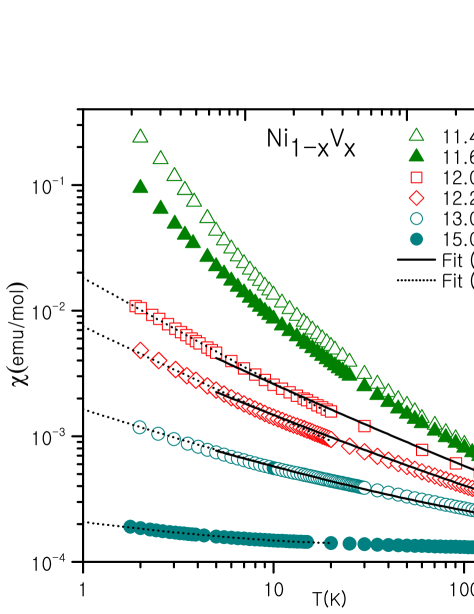
Figure 1: (Color online). Temperature dependence of the susceptibility of ${\rm{Ni}}_{x}{\rm{V}}_{1-x}$ for different Vanadium concentrations. Solid and dotted lines represent fits to Eq. (26) in the different temperature ranges 5 to 300 K and 1 to 20 K, respectively (data from Ref. Ubaid-Kassis et al., 2010).

Recently, indications of a quantum Griffiths phase have been observed in the transition metal ferromagnet ${\rm{Ni}}_{x}{\rm{V}}_{1-x}$. Ubaid-Kassis et al. (2010); Schroeder et al. (2011) The behavior of the thermodynamics has been described well in terms of the power-low quantum Griffiths singularities predicted for an itinerant antiferromagnet (and the transverse-field Ising model). Here, we compare our new theory of ferromagnetic quantum Griffiths phases with the experimental data given in Refs. Ubaid-Kassis et al., 2010; Schroeder et al., 2011. The residual resistivity of ${\rm{Ni}}_{x}{\rm{V}}_{1-x}$ close to the quantum phase transition is rather high. Thus, we choose $a=2$ for a diffusive ferromagnet. Figure 1 shows the behavior of the susceptibility as a function of temperature. The curves corresponding to the concentrations $x=13.0\%$ and $x=15.0\%$ (which are far away from the critical concentration $x_{c}\approx 11.5\%$) are described better by power laws rather than our modified quantum Griffiths behavior Eq. (26), at least above $T\approx 10\rm{K}$ (the low-temperature upturn is likely due to freezing of the rare regions). For concentrations $x=12.07\%$ and $x=12.25\%$, our theory fits better than power-law Griffiths singularities and extends the fit range from 30–300K down to 5–300K. The curves corresponding to the concentrations $x=11.4\%$ and $x=11.6\%$ can be fitted by Griffiths power-laws only in the temperature range 30 to 300 K, our new functional form Eq. (26) does not improve the fit of these curves.

We also compared the prediction Eq. (28) for a modified magnetization-field curve with the data given in Refs. Ubaid-Kassis et al., 2010; Schroeder et al., 2011. We found that the fits to power-laws and to the modified quantum Griffiths behavior Eq. (28) cannot be distinguished.

Let us also point out that the susceptibility data in the temperature range below 20K can be fitted reasonable well by Eq. (26); see details in Fig. 1. Further experiments may be necessary to decide whether our theory applies in this region.

Overall, our theory does not significantly improve the description of the data of Refs. Ubaid-Kassis et al., 2010; Schroeder et al., 2011 over the temperature range where Griffiths behavior is observed. A possible reason is that the relevant rare regions are too small. At concentrations $x=13.0\%$ and $x=15.0\%$, they have moments of about $\mu\approx 5\mu_{\rm{B}}$ and $\mu\approx 1\mu_{\rm{B}}$, respectively. Correspondingly, the effect of the order parameter transport cannot play any role, whereas our functional forms arise for large rare regions where the order parameter transport limits the relaxation of the rare region. A possible reason why the curves corresponding to the concentrations $x=11.4\%$ and $x=11.6\%$ can not be described by our theory at $T<30\rm{K}$ might be that the curves are actually slightly on the ordered side of the quantum phase transition.

VI Conclusions

In summary, we studied the dynamics of rare regions in disordered metals close to the ferromagnetic quantum phase transition, considering the cases of both Ising and Heisenberg spin symmetries. The overall phenomenology is similar to the well-studied antiferromagnetic quantum Griffiths behavior. Castro Neto and Jones (2000); Millis et al. (2002); Vojta (2003); Vojta and Schmalian (2005) Namely, for Ising symmetry at low temperatures, the overdamping causes sufficiently large rare regions to stop tunneling. Instead, they behave classically, leading to super-paramagnetic behavior and a smeared quantum phase transition. In contrast, at higher temperatures but below a microscopic cutoff scale, the damping is unimportant and quantum Griffiths singularities can be observed. In contrast to the Ising case, the itinerant Heisenberg ferromagnet displays quantum Griffiths singularities when damping is sufficiently strong, i.e., at low temperatures. Above a crossover temperature, conventional behavior is expected.

Although the phenomenologies of the ferro- and antiferromganetic cases are similar, the functional forms of the quantum Griffiths singularities are different. In ferromagnetic quantum Griffiths phases, the tunneling rate (or characteristic energy) of a rare region decays as $\exp[-{\rm{const.}}\times\gamma L^{a+3}]$ with its linear size $L$, where $a$ is equal to 1 or 2 for ballistic and diffusive ferromagnets, respectively. This leads to the modified nonpower-law quantum Griffiths singularities in thermodynamic quantities, discussed in Sec. IV, in contrast to the power-law quantum Griffiths singularities in itinerant antiferromagnets. The reason is the following. Because of the order parameter conservation in the itinerant quantum ferromagnet, the damping effects are further enhanced as the dimensionless dissipation strength $\alpha$ for a rare region of linear size $L$ is proportional to $L^{a+3}$ rather than $L^{3}$.

In strongly disordered system, where our theory is most likely to apply, the motion of the electron is diffusive. Correspondingly, we expect $a=2$. In hypothetical systems with rare regions, but ballistic dynamics of the electrons, $a$ would take the value 1.

In our explicit calculations, we have used Hertz’s form Hertz (1976) of the order-parameter field theory of the itinerant ferromagnetic quantum phase transition. However, mode-coupling effects in the Fermi liquid lead to an effective long-range spatial interaction between the order parameter fluctuations. Kirkpatrick and Belitz (1996); Vojta et al. (1996, 1997) In the order-parameter field theory, this leads to a nonanalytic momentum dependence of the static action Eq. (II). The effects of this long-range interaction on the existence and energetics of a locally ordered rare region were studied in detail in Ref. Hoyos and Vojta, 2007. This work showed that the long-range interactions only produce subleading corrections to the droplet-free energy. Therefore, including these long-range interactions in the action Eq. (1) will not change the results of the present paper.

Let us now turn to the limitations of our theory. In our calculations, we assumed that the droplet maintains its shape while collapsing and reforming. Correspondingly, our calculation provides a variational upper bound for the instanton action. There could be faster relaxation processes; however, it is hard to image the droplet dynamics to avoid the restriction coming from the order parameter conservation. We treated the individual, locally ordered rare regions as independent. But, in a real metallic magnet, they are weakly coupled by a Ruderman-Kittel-Kasuya-Yosida (RKKY), interaction which is not included in the Landau-Ginzburg-Wilson action Eq. (1). At the lowest temperatures, this RKKY interactions between the rare regions induces a cluster glass phase. Dobrosavljević and Miranda (2005) Finally, our theory does not take the feedback of the order parameter fluctuations on the fermions into account. It has been found that for some quantum phase transitions, the Landau-Ginzburg-Wilson theory breaks down sufficiently close to the transition point due to this feedback. Abanov et al. (2003); Belitz et al. (2005) For strongly disordered systems, this question has not been addressed yet, it remains a task for the future.

Turning to experiment, our theory does not significantly improve the description of the data of ${\rm{Ni}}_{x}{\rm{V}}_{1-x}$. Ubaid-Kassis et al. (2010); Schroeder et al. (2011) We believe that the main reason is that our theory is valid for asymptomatically large rare regions where the order parameter transport plays an important role, whereas the experimental accessible rare regions in ${\rm{Ni}}_{x}{\rm{V}}_{1-x}$ are not large enough for the order parameter conservation to dominate their dynamics. We expect our theory can be applied in systems where one can observe Griffiths singularities at lower temperatures leading to larger rare regions.

*

Appendix A Renormalization group theory

In this Appendix, we show the derivation of Eqs. (19) and (21) by renormalization group (RG) analysis. At low temperatures, the action Eq. (18) is formally equivalent to a quantum non-linear sigma model Nelson and Pelcovits (1977) in imaginary time $\tau$. We can set $\bf{n}(\tau)=(\pi(\tau),\sigma(\tau))$, where ${\pi}(\tau)=(\pi_{1}(\tau),\pi_{2}(\tau))$ represents transverse fluctuations. After expanding in $\pi$ and keeping terms up to $\mathcal{O}(g^{-2})$, $\mathcal{O}(\alpha^{-2})$, we find Nelson and Pelcovits (1977)

$$S=\int\frac{d\omega}{2\pi}\ \left(g\omega^{2}+\frac{\alpha}{4}|\omega|\right)|\tilde{\pi}(\omega)|^{2}+\int\frac{d\omega_{1}d\omega_{2}d\omega_{3}}{(2\pi)^{3}}\left(\frac{\alpha}{8}|\omega_{1}|-g\omega_{1}\omega_{3}\right)\tilde{\pi}_{\beta}(\omega_{1})\tilde{\pi}_{\beta}(\omega_{2})\tilde{\pi}_{\beta^{\prime}}(\omega_{3})\tilde{\pi}_{\beta^{\prime}}(-\omega_{1}-\omega_{2}-\omega_{3})\,.$$ (33)

We now consider the case of the small damping $\alpha\ll g$. Two different energy regimes can be distinguished: (i) $\omega$ larger than some crossover energy $\omega_{c}\sim\alpha/g$, implying that the undamped dynamics dominates the systems properties, and (ii) $\omega\ll\omega_{c}$, when the damping term is dominant.

(i) Because the contribution of the undamped dynamics is dominant in this regime, we neglect the damping term and renormalize $g$. To construct a perturbative renormalizaition group, consider a frequency region $[-\Lambda,\Lambda]$ ($\Lambda$ is a high energy cut off), and divide the modes into slow and fast ones, $\tilde{\pi}(\omega)=\tilde{\pi}^{<}(\omega)+\tilde{\pi}^{>}(\omega)$. The modes $\tilde{\pi}^{<}(\omega)$ involve frequency $-\Lambda/b<\omega<\Lambda/b$, and are kept. We integrate out the short-wavelength fluctuations $\pi^{>}(\omega)$ (with frequencies in the region $-\Lambda<\omega<-\Lambda/b$ and $\Lambda/b<\omega<\Lambda$) in perturbation theory using the propagator ${\langle\tilde{\pi}^{>}_{\beta}(\omega)\tilde{\pi}^{>}_{\beta^{\prime}}(\omega^{\prime})\rangle}={\pi\delta_{\beta\beta^{\prime}}\delta(\omega+\omega^{\prime})}/({g\omega^{2}})$.

After applying standard techniques, we find that this coarse graining changes the coupling constant $g$ to $g_{\rm{co}}=g+I_{g}(b)$, where $I_{g}(b)=(2\pi\Lambda)^{-1}(b-1)$. After rescaling $\tau^{\prime}=\tau/b$ and renormalizing $\pi^{\prime}(\tau^{\prime})=\pi^{<}(\tau)/\zeta_{g}$, we obtain the renormalized coupling constant in the form

$$g^{\prime}=b^{-1}\zeta^{2}_{g}g_{\rm{co}}\,.$$ (34)

To find the rescaling factor $\zeta_{g}$, we average ${\mathbf{n}}$ over the short wavelength modes $\pi^{>}$ and obtain

$$\langle{\bf{n}}\rangle^{>}= \langle(\pi^{<}_{1}+\pi^{>}_{1},...,\sqrt{1-(\pi^{<}+\pi^{>})^{2}})\rangle^{>}$$

$$= (1-\langle(\pi^{>})^{2}\rangle^{>}/2+\mathcal{O}(g^{-2}))(\pi^{<}_{1},...,\sqrt{1-(\pi^{<})^{2}})\,.$$ (35)

Thus, we identify

$$\zeta_{g}=1-\langle(\pi^{>})^{2}\rangle^{>}/2+\mathcal{O}(g^{-2})=1-\frac{I_{g}(b)}{g}+\mathcal{O}(g^{-2})\,.$$ (36)

Correspondingly, the renormalized coupling constant given in Eq. (34) becomes

$$g^{\prime}=b^{-1}(g-I_{g}(b))\,.$$ (37)

Setting $b=1+\delta l$, and integrating Eq. (37) gives the recursion relation $g(l)=g(0)e^{-l}$. To find the relaxation time, we run the RG to $g(l)=1$ and use $\xi^{{\tau}}\sim e^{l}$. This gives

$$\xi^{{\tau}}_{g}\sim L^{3}\,.$$ (38)

(ii) In the same way, for low energies $\omega\ll\omega_{c}$, we neglect the term corresponding to the undamped dynamics and renormalize the $\alpha$ coefficient. We find that $\alpha$ is not modified by the perturbation, i.e., $\alpha_{\rm{co}}=\alpha$, and the field rescaling factor $\zeta_{\alpha}$ is given by

$$\zeta_{\alpha}=1-\frac{I_{\alpha}(b)}{\alpha}+\mathcal{O}(\alpha^{-2})\,,$$ (39)

where $I_{\alpha}(b)=2\pi^{-1}\log(b)$. Then, we find the recursion relation ${\alpha}(l)={\alpha}(0)-4\pi^{-1}l$. This leads to the relaxation time

$$\xi^{{\tau}}_{\gamma}\sim\exp[{{\rm{const.}}\times\gamma L^{3+a}}]\,.$$ (40)

References

- Griffiths (1969) R. B. Griffiths, Phys. Rev. Lett. 23, 17 (1969).
- Thill and Huse (1995) M. Thill and D. A. Huse, Physica A 214, 321 (1995).
- Rieger and Young (1996) H. Rieger and A. P. Young, Phys. Rev. B 54, 3328 (1996).
- Fisher (1992) D. S. Fisher, Phys. Rev. Lett. 69, 534 (1992).
- Fisher (1995) D. S. Fisher, Phys. Rev. B 51, 6411 (1995).
- Vojta (2003) T. Vojta, Phys. Rev. Lett. 90, 107202 (2003).
- Vojta (2006) T. Vojta, J. Phys. A 39, R143 (2006).
- Vojta (2010) T. Vojta, J. Low Temp. Phys. 161, 299 (2010).
- Rogachev and Bezryadin (2003) A. Rogachev and A. Bezryadin, Appl. Phys. Lett. 83, 512 (2003).
- Löhneysen et al. (1994) H. V. Löhneysen, T. Pietrus, G. Portisch, H. G. Schlager, A. Schörder, M. Sieck, and T. Trappmann, Phys. Rev. Lett. 72, 3262 (1994).
- Grigera et al. (2001) S. A. Grigera, R. S. Perry, A. J. Schofield, M. Chiao, S. R. Julian, G. G. Lonzarich, S. I. Ikeda, Y. Maeno, A. J. Millis, and A. P. Mackenzie, Science 294, 329 (2001).
- Pfleiderer et al. (1997) C. Pfleiderer, G. J. McMullan, S. R. Julian, and G. G. Lonzarich, Phys. Rev. B 55, 8330 (1997).
- de Andrade et al. (1998) M. C. de Andrade, R. Chau, R. P. Dickey, N. R. Dilley, E. J. Freeman, D. A. Gajewski, M. B. Maple, R. Movshovich, A. H. Castro Neto, G. Castilla, and B. A. Jones, Phys. Rev. Lett. 81, 5620 (1998).
- Castro Neto and Jones (2000) A. H. Castro Neto and B. A. Jones, Phys. Rev. B 62, 14975 (2000).
- Vojta and Schmalian (2005) T. Vojta and J. Schmalian, Phys. Rev. B 72, 045438 (2005).
- Guo et al. (2008) S. Guo, D. P. Young, R. T. Macaluso, D. A. Browne, N. L. Henderson, J. Y. Chan, L. L. Henry, and J. F. DiTusa, Phys. Rev. Lett. 100, 017209 (2008).
- Guo et al. (2010a) S. Guo, D. P. Young, R. T. Macaluso, D. A. Browne, N. L. Henderson, J. Y. Chan, L. L. Henry, and J. F. DiTusa, Phys. Rev. B 81, 144423 (2010a).
- Guo et al. (2010b) S. Guo, D. P. Young, R. T. Macaluso, D. A. Browne, N. L. Henderson, J. Y. Chan, L. L. Henry, and J. F. DiTusa, Phys. Rev. B 81, 144424 (2010b).
- Sereni et al. (2007) J. G. Sereni, T. Westerkamp, R. Küchler, N. Caroca-Canales, P. Gegenwart, and C. Geibel, Phys. Rev. B 75, 024432 (2007).
- Westerkamp et al. (2009) T. Westerkamp, M. Deppe, R. Küchler, M. Brando, C. Geibel, P. Gegenwart, A. P. Pikul, and F. Steglich, Phys. Rev. Lett. 102, 206404 (2009).
- Ubaid-Kassis et al. (2010) S. Ubaid-Kassis, T. Vojta, and A. Schroeder, Phys. Rev. Lett. 104, 066402 (2010).
- Schroeder et al. (2011) A. Schroeder, S. Ubaid-Kassis, and T. Vojta, J. Phys. Condens. Matter 23, 094205 (2011).
- Hertz (1976) J. Hertz, Phys. Rev. B 14, 1165 (1976).
- Millis (1993) A. J. Millis, Phys. Rev. B 48, 7183 (1993).
- Note (1) We set Planck’s constant and Boltzmann constant to unity () in what follows.
- Millis et al. (2001) A. J. Millis, D. K. Morr, and J. Schmalian, Phys. Rev. Lett. 87, 167202 (2001).
- Millis et al. (2002) A. J. Millis, D. K. Morr, and J. Schmalian, Phys. Rev. B 66, 174433 (2002).
- Hoyos and Vojta (2007) J. A. Hoyos and T. Vojta, Phys. Rev. B 75, 104418 (2007).
- Legget et al. (1987) A. J. Legget, S. Chakravarty, A. T. Dorsey, M. P. A. Fisher, A. Garg, and W. Zwerger, Rev. Mod. Phys. 59, 1 (1987).
- Vojta et al. (2009) T. Vojta, C. Kotabage, and J. A. Hoyos, Phys. Rev. B 79, 024401 (2009).
- Moriya (1963) T. Moriya, J. Phys. Soc. Jpn. 18, 516 (1963).
- Note (2) A. Schroeder, private communications.
- Kirkpatrick and Belitz (1996) T. R. Kirkpatrick and D. Belitz, Phys. Rev. B 53, 14364 (1996).
- Vojta et al. (1996) T. Vojta, D. Belitz, R. Narayanan, and T. R. Kirkpatrick, Europhys. Lett. 36, 191 (1996).
- Vojta et al. (1997) T. Vojta, D. Belitz, R. Narayanan, and T. R. Kirkpatrick, Z. Phys. B 103, 451 (1997).
- Dobrosavljević and Miranda (2005) V. Dobrosavljević and E. Miranda, Phys. Rev. Lett. 94, 187203 (2005).
- Abanov et al. (2003) A. Abanov, A. V. Chubukov, and J. Schmalian, Adv. Phys. 52, 119 (2003).
- Belitz et al. (2005) D. Belitz, T. R. Kirkpatrick, and T. Vojta, Rev. Mod. Phys. 77, 579 (2005).
- Nelson and Pelcovits (1977) D. R. Nelson and R. A. Pelcovits, Phys. Rev. B 16, 2191 (1977).