Temporal disorder in up-down symmetric systems

Abstract

The effect of temporal disorder on systems with up-down Z2 symmetry is studied. In particular, we analyze two well-known families of phase transitions: the Ising and the generalized voter universality classes, and scrutinize the consequences of placing them under fluctuating global conditions. We observe that variability of the control parameter induces in both classes “Temporal Griffiths Phases” (TGP). These recently-uncovered phases are analogous to standard Griffiths Phases appearing in systems with quenched spatial disorder, but where the roles of space and time are exchanged. TGPs are characterized by broad regions in parameter space in which (i) mean first-passage times scale algebraically with system size, and (ii) the system response (e.g. susceptibility) diverges. Our results confirm that TGPs are quite robust and ubiquitous in the presence of temporal disorder. Possible applications of our results to examples in ecology are discussed.

I Introduction

Systems with up-down $Z_{2}$ symmetry –including the Ising model– are paradigmatic in Statistical Mechanics. Some of them –such as the voter model– exhibit absorbing states, a distinctive feature of non-equilibrium dynamics hinri ; odor ; GG ; marro . Absorbing states are configurations of the system characterized by the lack of fluctuations, where the dynamics becomes frozen and the system remains trapped. In the last years, a great interest has been given to this class of models with two symmetric absorbing states hinri ; odor ; GG ; marro ; alhammal1 ; dornic ; lipowski ; droz ; Vazquez-2008 ; Blythe , which are of high relevance in diverse problems in the ecological, biological, and social sciences, such as species competition spcomp , neutral theories of biodiversity Durret , allele frequency in genetics allele , opinion formation opinion , epidemics propagation Pinto , or language spreading language .

Phase transitions into absorbing states are quite universal. Systems exhibiting one absorbing state belong generically to the very robust Directed Percolation (DP) universality class and share the same set of critical exponents, amplitude ratios, and scaling functions. When this general rule is broken it is so owing to the presence of some additional symmetry or conservation law hinri ; odor ; GG ; marro . This is the case of the class of systems with $Z_{2}$-symmetric absorbing states, which may exhibit a phase transition with critical scaling differing from DP, usually referred as Generalized voter (GV), also called “parity conserving”, “DP2” or “directed Ising”, universality class (see hinri ; odor ; dornic and references therein). Analytical and numerical studies dornic ; droz ; alhammal1 ; Vazquez-2008 ; Blythe have shown that, depending on some details, $Z_{2}$-symmetric models may undergo either a unique GV-like phase transition separating an active/symmetric phase from an absorbing one or, alternatively, such a transition can split into two separate ones: an Ising-like transition in which the $Z_{2}$ symmetry is broken, and a second DP-like transition below which the broken-symmetry phase collapses into the corresponding absorbing state. In particular, a general stochastic theory, aimed at capturing the phenomenology of these systems, was proposed in alhammal1 ; depending on general features it may exhibit a DP, an Ising, or a GV transition.

In many situations, $Z_{2}$ symmetric systems are not isolated but, instead, affected by external conditions or by environmental fluctuations. The question of how external variability affects diversity, robustness, and evolution of complex systems, is of outmost relevance in different contexts. Take, for instance, the example of the neutral theory of biodiversity: if there are two $Z_{2}$-symmetric (or neutral) species competing, what happens if depending on environmental conditions one of the two species is favored at each time step in a symmetric way? Does such environmental variability enhance species coexistence or does it hinder it? Leigh ; Chesson ; Calabrese-2010 ; Vazquez-2010 ; dOdorico2009 .

Motivated by these questions, we study how basic properties of $Z_{2}$ symmetric systems, such as response functions and first-passage times, are affected by the presence of temporal disorder.

Some previous works have explored the effects of fluctuating global conditions in simple models exhibiting phase transitions jensen ; alonso ; kamenev . Temporal disorder has been shown to be a highly relevant perturbation around DP phase transitions in all dimensions (in apparent contradiction with the Harris criterion for the relevance of disorder jensen ), while temporal disorder has been shown to be relevant at the Ising transition only at and above three dimensions. More recently, a modified version of the simplest representative of the DP class –i.e. the Contact-Process– equipped with temporal disorder was studied in Vazquez-2011 . In this model, the control parameter (birth probability) was taken to be a random variable, varying at each time unit. As the control parameter is allowed to take values above and below the transition point of the pure contact process, the system alternates between the tendencies to be active or absorbing. As shown in Vazquez-2011 this dynamical frustration induces a logarithmic type of finite-size scaling at the transition point and generates a subregion in the active phase characterized by a generic algebraic scaling (rather than the usual exponential, Kramers-like, behavior) of the extinction times with system size. More strikingly, this subregion is also characterized by generic divergences in the system susceptibility, a property which is reserved for critical points in pure systems. This phenomenology is akin to the one in systems with quenched “spatial” disorder Vojta-2006 , which show algebraic relaxation of the order parameter, and singularities in thermodynamic potentials in broad regions of parameter space: the so-called, Griffiths Phases griffiths . The remarkable peculiarities of standard Griffiths phases stem from the existence of (exponentially) rare –locally ordered– regions which take a (exponentially) long time to decay, inducing an anomalously slow decay in the disordered phase.

In the case of temporal disorder, an analogy with Griffiths phases can be made, in the sense that very long (exponentially rare) time intervals (corresponding to an absorbing phase of the pure model) of the control parameter have a large influence on the system dynamics even when the overall system is in its active phase. These phenomenological similarities between systems with spatial and temporal disorder led us to introduce the concept of “Temporal Griffiths Phases” (TGP) Vazquez-2011 .

In order to investigate whether the anomalous behavior that leads to TGPs around absorbing state (DP) phase transitions is a universal property of systems in other universality classes –and in particular, in up-down symmetric systems– we study the possibility of having TGPs around Ising and GV transitions. We scrutinize simple models in these two classes and assume that the corresponding control parameter changes randomly in time, fluctuating around the transition point of the corresponding pure model, and study the susceptibility as well as mean-first passage times. We mainly focus on the mean-field (high dimensional) limit, since it allows for analytical treatment via a Langevin approach, but we also provide numerical results and some theoretical considerations for low dimensional systems.

The paper is organized as follows. In section II, we develop a general mean-field description of models with varying control parameters in terms of collective variables. In section III and IV, we show analytical and numerical results for the Ising and GV transitions, respectively. In section V, a short summary and conclusions are presented.

II Mean-field theory of $Z_{2}$-symmetric models with temporal disorder

Interacting particle models evolve stochastically over time. A useful technique to study such systems is the mean-field (MF) approach, which implicitly assumes a “well-mixed” situation, where each particle can interact with any other, providing a sound approximation in high dimensional systems. One way in which the mean-field limit can be seen at work is by analyzing a fully connected network (FCN), where each node (particle) is directly connected to any other else, mimicking an infinite dimensional system.

In the models we study here, states can be labeled with occupation-number variables $\rho_{i}$ taking a value $1$ if node $i$ is occupied or $0$ if it is empty, or alternatively by spin variables $S_{i}=2\rho_{i}-1$, with $S_{i}=\pm 1$. Using these latter, the natural order parameter is the magnetization per spin, defined as

$$m=\frac{1}{N}\sum_{i=1}^{N}S_{i},$$ (1)

where $N$ is the total number of particles in the system. The master equation for the probability $P(m,t)$ of having magnetization $m$ at a given time $t$, is

$$P(m,t+1/N) = \omega_{+}\left(m-2/N,b\right)P\left(m-2/N,t\right)$$

$$+ \omega_{-}\left(m+2/N,b\right)P\left(m+2/N,t\right)$$

$$+ \left[1-\omega_{-}(m,b)-\omega_{+}(m,b)\right]P(m,t),$$

where $\omega_{\pm}(m,b)$ are the transition probabilities from a state with magnetization $m$ to a state with magnetization $m\pm 2/N$. This describes a process in which a “spin” is randomly selected at every time-step (of length $dt=1/N$), and inverted with a probability that depends on $m$ and the control parameter $b$. The allowed magnetization changes in an individual update, $\Delta m=\pm 2/N$, are infinitesimally small in the $N\rightarrow\infty$ limit. In this limit, one can perform a standard Kramers-Moyal expansion vanKampen ; Gardiner leading to the Fokker-Planck equation

$$\frac{\partial P(m,t)}{\partial t}=-\frac{\partial}{\partial m}\left[f(m,b)P(m,t)\right]+\frac{1}{2}\frac{\partial^{2}}{\partial m^{2}}\left[g(m,b)P(m,t)\right],$$ (3)

with drift and diffusion terms given, respectively, by

$$f(m,b) = 2\left[\omega_{+}(m,b)-\omega_{-}(m,b)\right],$$ (4)

$$g(m,b) = \frac{4\left[\omega_{+}(m,b)+\omega_{-}(m,b)\right]}{N}.$$ (5)

From Eq. (3), and working in the Itô scheme (as justified by the fact that it comes from a discrete in time equation horsthemke ), its equivalent Langevin equation is Gardiner

$$\dot{m}=f(m,b)+\sqrt{g(m,b)}\,\eta(t),$$ (6)

where the dot stands for time derivative, and $\eta(t)$ is a Gaussian white noise of zero-mean and correlations $\langle\eta(t)\eta(t^{\prime})\rangle=\delta(t-t^{\prime})$. The diffusion term is proportional to $1/\sqrt{N}$, and therefore, it vanishes in the thermodynamic limit ($N\to\infty$), leading to a deterministic equation for $m$.

The drift and diffusion coefficients in Eq. (6) depend not only on the magnetization, but also on the parameter $b$. To analyze the behavior of the system when $b$ changes randomly over time, and following previous works Vazquez-2010 ; Vazquez-2011 , we allow $b$ to take a new random value, extracted from a uniform distribution, in the interval $(b_{0}-\sigma,b_{0}+\sigma)$ at each MC step, i.e., every time interval $\tau=1$. Thus, we assume that the dynamics of $b(t)$ obeys an Ornstein-Uhlenbeck process

$$b(t)=b_{0}+\sigma\,\xi(t),$$ (7)

where $\xi(t)$ is a step-like function that randomly fluctuates between $-1$ and $1$, as depicted in Fig. 1a. Its average correlation is

$$\overline{<\xi(t)\xi(t+\Delta t)>}=\left\{\begin{array}[]{ll}\frac{1}{3}(1-|\Delta t|/\tau)&\mbox{for $|\Delta t|<\tau$}\\ \\ 0&\mbox{for $|\Delta t|>\tau$,}\end{array}\right.$$ (11)

where the bar stands for time averaging. The parameters $b_{0}$ and $\sigma$ are chosen with the requirement that $b$ takes values at both sides of the transition point of the pure model (see Fig. 1b), that is, the model with constant $b$. Thus, the system randomly shifts between the tendencies to be in one phase or the other (see Fig. 2).

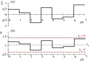
Figure 1: (Color online). (a) Typical realization of the colored noise $\xi(t)$, a step like function that takes values between $+1$ and $-1$. (b) Stochastic control parameter $b(t)=b_{0}+\sigma\xi(t)$ according to the values of the noise in (a), $b_{0}=1.03$ and $\sigma=0.4$.

The model presents both intrinsic and extrinsic fluctuations, as represented by the white noise $\eta(t)$ and the colored noise $\xi(t)$, respectively. Plugging the expression Eq.  (7) for $b(t)$ into Eq. (6), and retaining only linear terms in the noise one readily obtains

$$\dot{m}=f_{0}(m)+\sqrt{g_{0}(m)}\,\eta(t)+j_{0}(m)\,\xi(t),$$ (12)

where $f_{0}(m)\equiv f(m,b_{0})$, $g_{0}(m)\equiv g(m,b_{0})$ and $j_{0}(m)$ is a function determined by the functional form of $f(m,b)$, that might also depend on $b_{0}$. To simplify the analysis, we assume that relaxation times are much longer than the autocorrelation time $\tau$, and thus take the limit $\tau\to 0$ in the correlation function Eq. (11), and transform the external colored noise $\xi$ into a Gaussian white noise with effective amplitude $K\equiv\int_{-\infty}^{+\infty}\overline{<\xi(t)\xi(t+\Delta t)>}\,d\Delta t=\tau/3$. Then, we combine the two white noises into an effective Gaussian white noise, whose square amplitude is the sum of the squared amplitudes of both noises Gardiner , and finally arrive at

$$\dot{m}=f_{0}(m)+\sqrt{g_{0}(m)+Kj_{0}^{2}(m)}\,\gamma(t),$$ (13)

where $\langle\gamma(t)\rangle=0$ and $\langle\gamma(t)\gamma(t^{\prime})\rangle=\delta(t-t^{\prime})$.

In the next two sections, we analyze the dynamics of the kinetic Ising model with Glauber dynamics and a variation of the voter model (the, so-called, q-voter model) –which are representative of the Ising and GV transitions respectively– in the presence of external noise. For that we follow the strategy developed in this section to derive mean-field Langevin equations and present also results of numerical simulations (for both finite and infinite dimensional systems), as well as analytical calculations.

III Ising transition with temporal disorder

We consider the kinetic Ising model with Glauber dynamics Glauber-1969 , as defined by the following transition rates

$$\Omega_{i}(S_{i}\rightarrow-S_{i})=\frac{1}{2}\left[1-S_{i}\,{\rm\tanh}\left(\frac{b}{2d}\sum_{j\in\langle i\rangle}S_{j}\right)\right].$$ (14)

The sum extends over the $2d$ nearest neighbors of a given spin $i$ on a $d$-dimensional hypercubic lattice, and $b=J\beta$ is the control parameter. $J$ is the coupling constant between spins, which we set to $1$ from now on, and $\beta=(k_{B}T)^{-1}$. Note that $b$ in this case is proportional to the inverse temperature.

III.1 The Langevin equation

In the mean-field case, the cubic lattice is replaced by a fully-connected network in which the number of neighbors $2d$ of a given site is simply $N-1$. Then, the transition rates of Eq. (14) can be expressed as

$$\Omega_{\pm}(m,b)\equiv\Omega(\mp\to\pm)=\frac{1}{2}\left[1\pm{\rm tanh}\left(b\,m\right)\right].$$ (15)

which implies $\omega_{\pm}(m,b)=\frac{1\mp m}{2}\,\Omega_{\pm}(m,b)$ for jumps in the magnetization. Following the steps in the previous section, and expanding $\Omega_{\pm}$ to third order in $m$, we obtain

$$\dot{m}=a_{0}m-c_{0}m^{3}+\sqrt{\frac{1-b_{0}m^{2}}{N}+K\sigma^{2}m^{2}(1-b_{0}^{2}m^{2})^{2}}\,\,\gamma(t),$$ (16)

where $b_{0}$ is the mean value of the stochastic control parameter, $a_{0}\equiv b_{0}-1$, and $c_{0}\equiv b_{0}^{3}/3$.

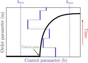
Figure 2: (Color online). Schematic representation of the fluctuating control parameter in the Ising model with Glauber dynamics. It makes the system shift between the ordered phase to the disordered one.

The potential $V(m)=-\frac{a_{0}}{2}m^{2}+\frac{c_{0}}{4}m^{4}$ associated with the deterministic term of Eq. (16) has the standard shape of the Ising class, that is, of systems exhibiting a spontaneous breaking of the $Z_{2}$ symmetry. A single minimum at $m=0$ exists in the disordered phase, while two symmetric ones, at $\pm\sqrt{a/c}$ exist below the critical point.

III.2 Numerical Results

In this section we study two magnitudes that were shown to be relevant in systems with temporal disorder Vazquez-2011 : the mean crossing time (or mean-first passage time) and the susceptibility. The crossing time is the time employed by the system to reach the disordered zero-magnetization state for the first time, starting from a fully ordered state with $|m|=1$ (see Fig. 3). Crossing times were calculated by numerically integrating Eq. (16) for different realizations of the noise $\gamma$ and averaging over many independent realizations. These integrations were performed using a standard stochastic Runge-Kutta scheme (note that, the noise term does not have any pathological behavior at $m=0$ as occurs in systems with absorbing states, for which more refined integration techniques are required Dornic ) . Results are shown in Fig. 4.

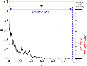
Figure 3: (Color online). Single realization of the stochastic process. The system starts with all the spins in the same state $(m=1)$ and the dynamics is stopped when it crosses $m=0$, which defines the crossing time in the Ising model. We take $\sigma=0.4$, $b_{0}=0.98$ and system size $N=10^{6}$. On the right margin we sketch the mapping of the problem to a Random Walk with jump length $|\Delta m|=2/N$.

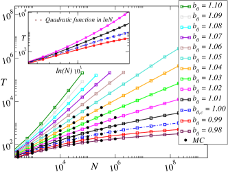
Figure 4: (Color online). Main: Log-log plot of the crossing time $T(N)$ for the Ising Model with Glauber dynamics in mean field. Values of the control parameter from $b_{0}=0.98$ (bottom) to $b_{0}=1.10$ (top) are shown. Monte Carlo simulations on a FCN (circles) and numerical integration of the Langevin equation Eq.  (16) with $\sigma=0.4$ (squares and interpolation with solid lines). There is a region with generic algebraic scaling of $T(N)$ and continuously varying exponents, $b_{0}\in[1.01,1.10]$. Inset: log-log plot of $T(N)$ vs. $\ln N$. At criticality (dotted-dashed line) the scaling is fitted to a quadratic function in $\ln N$.

To estimate the critical point, we calculated the time evolution of the average magnetization $\langle m\rangle(t)$ by integrating the Langevin equation Eq. (16), and also by performing Monte Carlo simulations of the particle system on a fully connected network. At the critical point $b_{0,c}$ the magnetization decays to zero as $\langle m\rangle\sim t^{-\beta}$. We have estimated $b_{0,c}=1$, which coincides with the pure case critical point $b_{c,pure}=1$: the critical point in the presence of disorder in mean-field is not shifted with respect to the pure system, in agreement with the analytical calculation in appendix A. At this critical point, as it is characteristic of TGPs Vazquez-2011 , a scaling of the form $T\sim[\ln N]^{\alpha}$ is expected. The numerically determined exponent value $\alpha\simeq 2.81$ for $\sigma=0.4$ is higher than the exponent $\alpha=2$ of the asymptotic analytical prediction Eq. (80), probably because of the asymptotic regime in $\ln N$ has not been reached. Instead, the behavior for arbitrary values of $N$ appears to be a second order polynomial in $\ln N$, as we can see in Eq. (71). Indeed, the numerical data is well fitted by the quadratic function $a\,(\ln N)^{2}+b\,\ln N+c$ (see inset of Fig. 4).This is to be compared with the standard power-law scaling $T\sim N^{\beta}$ characteristic of pure systems, i.e. for $\sigma=0$. Moreover, a broad region showing algebraic scaling $T\sim N^{\delta}$ with a continuously varying exponent $\delta(b_{0})$ ($\delta\rightarrow 0$ as $b_{0}\rightarrow b^{+}_{0,c}$) appears in the ordered phase $b_{0}>b_{0,c}$. Both $\alpha$ and $\delta$ are not universal and depend on the noise strength $\sigma$. Finally, in the disordered phase the scaling of $T$ is observed to be logarithmic, $T\sim\ln N$.

We have also performed Monte Carlo simulations of the time-disordered Glauber model on two- and three-dimensional cubic lattices with nearest neighbor interactions. The critical point was computed following standard methods, that is, by looking for a power law scaling of $\langle m\rangle$ versus time, as we mentioned above. In $d=2$, a shift in the critical point was found: from $b_{c,pure}=0.441(1)$ in the pure model to $b_{0,c}=0.605(1)$ for $\sigma=0.4$. However, the scaling behavior of $T$ with $N$ resembles that of the pure model, with $T\sim N^{\beta}$ at criticality (with an exponent numerically close to that of the pure model marro ), and an exponential growth $T\sim\exp(cN)$, where $c$ is a positive constant, in the ordered phase (Arrhenius law) ) (see Fig. 5). Thus, no region of generic algebraic scaling appears in this low-dimensional system. On the contrary, in $d=3$, results qualitatively similar to mean-field ones are recovered (see Fig. 6). The critical point is shifted from $b_{c,pure}=0.222(1)$ (calculated in heuer ) to $b_{0,c}=0.413(2)$, with a critical exponent $\alpha(d=3)=5.29$ for $\sigma=0.4$, and generic algebraic scaling in the ordered phase. In conclusion, our numerical studies suggest that the lower critical dimension for the TGPs in the Ising transition is $d_{c}=3$. This is in agreement with the analytical finding in alonso , establishing that temporal disorder is irrelevant in Ising-like systems below three dimensions. This result is to be compared with $d_{c}=2$ numerically reported for the existence of TGPs in DP-like transitions Vazquez-2011 (observe, however, that temporal disorder, in this case, affects the value of critical exponents at criticality in all spatial dimensions). Further studies are needed to clarify the relation between disorder-relevance at criticality and the existence or not of TGPs.

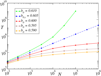
Figure 5: (Color online). Log-log plot of the crossing time $T(N)$ for the Ising Model with Glauber dynamics in $d=2$. Values of the control parameter from $b_{0}=0.590$ (bottom) to $b_{0}=0.610$ (top) are shown. Monte Carlo simulations on a regular cubic lattice with $\sigma=0.4$ (lines are interpolations). We observe a power law scaling at the critical point (dotted-dashed line). TGP are not observed, crossing time scales exponentially in the ordered phase (light green, upper, line).

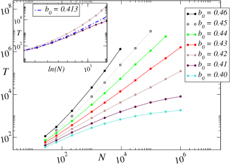
Figure 6: (Color online). Main: Log-log plot of the crossing time $T(N)$ for the Ising Model with Glauber dynamics in $d=3$. Monte Carlo simulations on a regular cubic lattice with $\sigma=0.4$ (lines are interpolations). Values of the control parameter from $b_{0}=0.40$ (bottom) to $b_{0}=0.46$ (top) are shown. There is a region $b\in[0.42,0.46]$ with generic algebraic scaling of $T(N)$ and continuously varying exponents. Inset: log-log plot of $T(N)$ vs. $\ln(N)$. It is estimated at criticality (dotted-dashed line) $T\sim(\ln N)^{5.29}$.

We have also measured the susceptibility $\chi$, defined as the response function to an external field $h$ in the vanishing field limit

$$\chi=\lim_{h\rightarrow 0}\frac{\partial\langle m\rangle}{\partial h},$$ (17)

where $\langle m\rangle$ denotes the stationary magnetization averaged over many independent realizations. In the presence of an external field, the transition rates become $\Omega_{\pm}(m,b)=\frac{1}{2}\left[1\pm{\rm tanh}\left(b\,m+h\right)\right]$. Expanding the hyperbolic tangent up to third order in $m$ and to first order in $h$, we obtain the following Langevin equation

$$\dot{m}=a_{0}m-c_{0}m^{3}+h\left(1-b^{2}m^{2}\right)+\sqrt{K}\sigma m(1-b_{0}^{2}m^{2})\,\,\gamma(t),$$ (18)

where we have considered the $N\to\infty$ limit $(g_{0}=0)$.

The average magnetization $\langle m\rangle$ for a given field $h$ was calculated by integrating the Langevin equation and then taking averages over noise realizations. The susceptibility can be computed, for different values of $b_{0}$, as the derivative of $\langle m\rangle$ with respect to $h$. Generic divergences of the form $\chi\sim h^{\upsilon}+\mbox{Constant}$ (with $\upsilon<0$ as $h\to 0$) appear in a broad region $b_{0}\in[b_{0,c}-\sigma^{2}/2,b_{0,c}+\sigma^{2}/2]$, centered around $b_{0,c}$, with symmetric exponents around the critical point (see Fig. 7). These results agree with those obtained through Monte Carlo simulations on a FCN (not shown). In finite dimensions, given the required large systems sizes and small fields, we could not conclude about the existence or not of generic divergences.

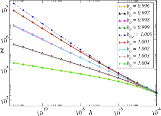
Figure 7: (Color online). Main: Log-log plot of the susceptibility as a function of the external field for different values of $b_{0}\in[b_{0,c}-\sigma^{2}/2,b_{0,c}+\sigma^{2}/2]$ with $\sqrt{K}\sigma=0.1$, obtained by integrating Eq. (18). Generic divergences with symmetric exponents around the critical value $b_{0.c}=1$ (dotted-dashed line) are observed.

III.3 Analytical results

Let us consider the Langevin equation Eq. (16) in the thermodynamic limit ($g_{0}(m)=0$). Given that the remaining intrinsic noise comes from a transformation of a colored noise into a white noise, the Stratonovich interpretation is to be used to obtain its associated Fokker-Planck equation (see e.g. horsthemke )

$$\frac{\partial P(m,t)}{\partial t} = -\frac{\partial}{\partial m}\Bigg{\{}\left[f_{0}(m)+\frac{K}{2}j_{0}(m)j^{\prime}_{0}(m)\right]P(m,t)\Bigg{\}}$$ (19)

$$+ \frac{1}{2}\frac{\partial^{2}}{\partial m^{2}}\Big{\{}Kj^{2}_{0}(m)P(m,t)\Big{\}}.$$

Imposing the detailed balance (fluxless) condition, it is straightforward to obtain the steady state solution

$$P_{st}(m)\propto\exp\left(-\frac{c_{0}m^{2}}{K\sigma^{2}}\right)|m|^{\frac{2a_{0}}{K\sigma^{2}}-1},$$ (20)

with a power-law singularity at the origin; this is a distinctive trait of a Langevin equation with linear multiplicative noise grinstein ; renmunoz . By performing a calculation analogous to that in Vazquez-2011 , we have analytically computed the system susceptibility and found that $\chi\sim h^{\upsilon}+\mbox{Constant}$, as mentioned earlier, and in agreement with previous results found in Vazquez-2011 ; grinstein ; renmunoz , with

$$\upsilon=\frac{2(b_{0}-1)}{K\sigma^{2}}-1.$$ (21)

This, in particular, implies that the susceptibility diverges when $\upsilon<0$ as $h\to 0$ or, in terms of the control parameter $b_{0}=1+a_{0}$, when $b_{0}$ takes a value in the region $1-\sigma^{2}/2<b_{0}<1+\sigma^{2}/2$ centered at the critical point $b_{0,c}=1$. The values of the exponent $\upsilon$ agree well with those of Fig. 7 at some distance from the critical point. For instance, an analytical value $\upsilon=-0.40$ for $b_{0}=1.003$ corresponds to a numerical value $\upsilon_{num}=-0.39$, and $\upsilon=-0.60$ for $b_{0}=-1.002$ to a value $\upsilon_{num}=-0.59$. However, the analytical exponent $\upsilon=-1$ at the critical point is not in good agreement with the numerical result $\upsilon_{num}=-0.88$, indicating that the asymptotic regime has not been numerically reached.

We next provide analytical results for the crossing time. Starting from the N-independent Fokker-Planck equation Eq. (19), an effective dependence on $N$ is implemented by calculating the first-passage time to the state $m=|2/N|$ rather than $m=0$. This is equivalent to the assumption that the system reaches the zero magnetization state with an equal number $N_{+}=N_{-}=N/2$ of up and down spins when $|m|<2/N$, that is, when $N/2-1<N_{+}<N/2+1$. The mean-first passage time $T$ associated with the Fokker-Planck equation Eq. (19) obeys the differential equation Gardiner

$$\frac{K}{2}j^{2}_{0}(m)T^{\prime\prime}(m)+\left[f_{0}(m)+\frac{K}{2}j_{0}(m)j^{\prime}_{0}(m)\right]T^{\prime}(m)=-1,$$ (22)

with absorbing and reflecting boundaries at $|m|=2/N$ and $|m|=1$, respectively. The solution, starting at time $t=0$ from $m=1$ is given by

$$T(m=1)=2\int_{2/N}^{1}\frac{dy}{\psi(y)}\int_{y}^{1}\frac{\psi(z)}{Kj_{0}^{2}(z)}dz,$$ (23)

where

$$\psi(x)=\exp\Bigg{\{}\int_{2/N}^{x}\frac{2f_{0}(x^{\prime})+Kj_{0}(x^{\prime})j^{\prime}_{0}(x^{\prime})}{Kj_{0}^{2}(x^{\prime})}dx^{\prime}\Bigg{\}}.$$ (24)

Computing these integrals (see Appendix A) we obtain

$$T\sim\left\{\begin{array}[]{ll}{\ln N}/(b_{0}-1)&\mbox{for $b_{0}<1$}\\ 3(\ln N)^{2}/\sigma^{2}&\mbox{for $b_{0}=1$}\\ N^{\frac{6(b_{0}-1)}{\sigma^{2}}}&\mbox{for $b_{0}>1$.}\end{array}\right.$$ (28)

These expressions qualitatively agree with the numerical results of Fig. 4, showing that $T$ grows logarithmically with $N$ in the absorbing phase $b_{0}<1$, as a power law in the active phase $b_{0}>1$, and as a power of $\ln N$ (i.e. poly-logarithmically) at the transition point $b_{0,c}=1$. The exponents $\delta=6(b_{0}-1)/\sigma^{2}$ do not agree well with the numerically determined exponents. This is probably due to to the fact that we have neglected the $1/\sqrt{N}$ term by taking $g_{0}=0$, which becomes of the same magnitude as the $j_{0}$ term when $|m|$ approaches $2/N$. Indeed, this was confirmed (not shown) by testing that analytical expressions Eq. (28) agree very well with numerical integrations of Eq. (16) performed for $g_{0}=0$, and setting the crossing point at $m=2/N$. In summary, this analytical approach reproduces qualitatively –and in some cases quantitatively– the above reported non-trivial phenomenology.

IV Generalized Voter transition with temporal disorder

We study in this section the GV transition dornic , which appears when a $Z_{2}$-symmetry system simultaneously breaks the symmetry and reaches one of the two absorbing states. A model presenting this type of transition is the nonlinear $q$-voter model, introduced in qvoter . The microscopic dynamics of this nonlinear version of the voter model consists in randomly picking a spin $S_{i}$ and flipping it with a probability that depends on the state of $q$ randomly chosen neighbors of $S_{i}$ (with possible repetitions). If all neighbors are at the same state, then $S_{i}$ adopts it with probability $1$ (which implies, in particular, that the two completely ordered configurations are absorbing). Otherwise, $S_{i}$ flips with a state-dependent probability

$$f(x,b)=x^{q}+b[1-x^{q}-(1-x)^{q}],$$ (29)

where $x$ is the fraction of disagreeing (antiparallel) neighbors and $b$ is a control parameter. Three types of transitions, Ising, DP and GV can be observed in this model depending on the value of $q$ qvoter . Here, we focus on the $q=3$ case, for which a unique GV transition at $b_{c}=1/3$ has been reported qvoter .

IV.1 The Langevin equation

In the MF limit (FCN) mf , the fractions of antiparallel neighbors of the two types of spins $S_{i}=1$ and $S_{i}=-1$ are $x=(1-m)/2$ and $x=(1+m)/2$, respectively. Thus, the transition probabilities are

$$\omega_{\pm}(m,b)=\frac{1\mp m}{2}\,f\left(\frac{1\pm m}{2},b\right).$$ (30)

Following the same steps as in the previous section, we obtain the Langevin equation

$$\dot{m}=\frac{1-3b_{0}}{2}m(1-m^{2})+$$

$$\sqrt{\frac{\left(1-m^{2}\right)(1+6b_{0}+m^{2})}{N}+\frac{9K}{4}\sigma^{2}m^{2}(1-m^{2})^{2}}\,\,\gamma(t).$$

Let us remark that the potential in the nonlinear voter model (Fig. 8) differs from that for the Ising model. Owing to the fact that the coefficients of the linear and cubic term in the deterministic part of Eq. (IV.1) coincide (except for their sign), the system exhibits a discontinuous jump at the transition point, where the potential minimum changes directly from $m=0$ in the disordered phase to $m=\pm 1$ in the ordered one. Furthermore, the potential vanishes at the critical point alhammal1 .

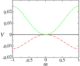
Figure 8: (Color online). Potential for the GV transition in a mean field approach. The dashed, solid and dot-dashed lines correspond to the paramagnetic phase, critical point, and the ferromagnetic phase, respectively.

IV.2 Numerical Results

The ordering time, defined as the averaged time required to reach a completely ordered configuration (absorbing state) starting from a disordered configuration, is the equivalent of the crossing time above. We have measured the mean ordering time $T$ by both, integrating the Langevin equation Eq. (IV.1) and running Monte Carlo simulations of the microscopic dynamics on FCNs and finite dimensions. In Fig. 9 we show the MF results. We observe that $T$ has a similar behavior to the one found for the mean crossing time in the Ising model, and for the mean extinction time for the contact process Vazquez-2011 . That is, a critical scaling $T\sim[\ln N]^{\alpha}$ at the transition point $b_{0,c}=1/3$, with a critical exponent $\alpha=3.68$ for $\sigma=0.3$, a logarithmic scaling $T\sim\ln N$ in the absorbing phase $b_{0}<b_{0,c}$, and a power law scaling $T\sim N^{\delta}$ with continuously varying exponent $\delta(b_{0})$ in the active phase $b_{0}>b_{0,c}$.

Monte Carlo simulations on regular lattices of dimensions $d=2$ and $d=3$ revealed that there is no significant change in the scaling behavior respect to the pure model (not shown). The critical point shifts in $d=2$ and remains very close to its mean-field value in $d=3$, but results are compatible with the usual critical (pure) voter scaling $T_{2d}\sim N\ln N$ and $T_{3d}\sim N$. In the absorbing phase $T$ grows logarithmically with $N$, while in the active phase $T$ grows exponentially fast with $N$, as in the pure-model case. Therefore, in these finite dimensional systems we do not find any TGP nor other anomalous effects induced by temporal disorder, although we cannot numerically exclude their existence in $d=3$. Such effects should be observable, only in higher dimensional systems (closer to the mean-field limit).

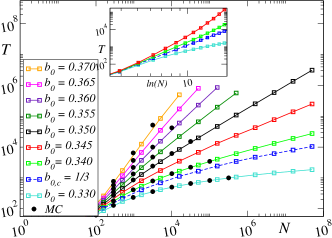
Figure 9: (Color online). Main: Log-log plot of the ordering time as a function of the system size $N$ in the MF q-voter model. Monte Carlo simulations on a FCN (dots) and numerical integration of the Langevin equation Eq.  (IV.1) for values of $b$ going from $0.330$ (bottom) to $0.370$ (top), and $\sigma=0.3$ (squares and solid lines interpolation). In the active phase a finite region with power law scaling is observed, $b_{0}\in[0.340,0.370]$. Inset: log-log plot of $T$ as a function of $\ln N$. At the critical point (dashed line) is $T\sim[\ln N]^{3.68}$.

IV.3 Analytical results

The ordering time $T$ can be estimated by assuming that the dynamics is described by the Langevin equation Eq. (IV.1), and calculating the mean first-passage time from $m=0$ to any of the two barriers located at $|m|=1$. It turns out useful to consider the density of up spins rather than the magnetization

$$\rho\equiv\frac{1+m}{2}.$$ (32)

$T$ is the mean first-passage time to $\rho=0$ starting from $\rho=1/2$. The Langevin equation for $\rho$ is obtained from Eq. (IV.1), by neglecting the $1/\sqrt{N}$ term and applying the ordinary transformation of variables (which is done employing standard algebra, given that Eq. (IV.1) is interpreted in the Stratonovich sense) is

$$\dot{\rho}=A(\rho)+\sqrt{K}C(\rho)\gamma(t),$$ (33)

with

$$A(\rho) = a_{0}\rho(2\rho-1)(1-\rho),$$

$$C(\rho) = 3\sigma\rho(2\rho-1)(1-\rho),$$ (34)

where $a_{0}=1-3b_{0}$.
Now, we can follow the same steps as in section III.3 for the Ising model, and find the equation for the mean first-passage time $T(\rho)$ by means of the Fokker-Planck equation. The solution is given by (see Appendix B)

$$T\sim\left\{\begin{array}[]{ll}{\ln N}/{\left(3b_{0}-1\right)}&\mbox{for $b_{0}<1/3$}\\ {(\ln N)^{2}}/{3\sigma^{2}}&\mbox{for $b_{0}=1/3$}\\ N^{\frac{2(b_{0}-1/3)}{\sigma^{2}}}&\mbox{for $b_{0}>1/3$.}\end{array}\right.$$ (38)

These scalings, which qualitatively agree with the numerical results of Fig. 9 for the $q$-voter, show that the behavior of $T$ is analogous to the one observed in the Ising transition of section III and in the DP transition found in Vazquez-2011 . Therefore, we conclude that TGPs appear around GV transitions in the presence of external varying parameters in high dimensional systems.

For the GV universality class the renormalization group fixed point is a non-perturbative one Canet , becoming relevant in a dimension between one and two. A field theoretical implementation of temporal disorder in this theory is still missing, hence, theoretical predictions and sound criteria for disorder relevance are not available.

V Summary and conclusions

We have investigated the effect of temporal disorder on phase transitions exhibited by $Z_{2}$ symmetric systems: the (continuous) Ising and (discontinuous) GV transitions which appear in many different scenarios. We have explored whether temporal disorder induces Temporal Griffiths Phases as it was previously found in standard (DP) systems with one absorbing state. By performing mean-field analyses as well as extensive computer simulations (in both fully connected networks and in finite dimensional lattices) we found that TGPs can exist around equilibrium (Ising) transitions (above $d=2$) and around discontinuous (GV) non-equilibrium transitions (only in high-dimensional systems). Therefore, we confirm that TGPs may also appear in systems with two symmetric absorbing states, illustrating the generality of the underlying mechanism: the appearance of a region, induced by temporal stochasticity of the control parameter, where first-passage times scale as power laws of the system size and where the susceptibility diverges. Temporal disorder, makes the ordered/active phase less stable and makes the system highly susceptible to perturbations. This appears to be a rather general and robust phenomenon.

It also seems to be a general property that TGPs do not appear in low dimensional systems, where standard fluctuations dominate over temporal disorder. In all the cases studied so far, a critical dimension $d_{c}$ –at and below which TGPs do not appear– exist ($d_{c}=1$ for DP transitions, $d_{c}=2$ for Ising like systems, and $d_{c}\simeq 3$ for GV ones). Calculating analytically such a critical dimension and comparing it with the standard critical dimension for the relevance/irrelevance of temporal disorder at the critical point (i.e. at the renormalization group non-trivial fixed point of the corresponding field theory) remains an open and challenging task.

A relevant application of our results is found in models of ecosystems. In this case, first-passage times are related to typical extinction times, and studying how such extinction times are affected by system size (e.g. habitat fragmentation) is a problem of outmost relevance. Future research might be oriented to the effect of temporal disorder on the formation and dynamics of spatial structures.

Appendix A Analytical calculations of the crossing time for the mean field Ising model

The mean first passage time to reach an absorbing barrier at $|m|=2/N$ starting from $|m|=1$ can be expressed as Gardiner ,

$$T(m=1)=2\int_{2/N}^{m=1}\frac{dy}{\psi(y)}\int_{y}^{1}\frac{\psi(z)}{Kj_{0}^{2}(z)}dz,$$ (39)

with

$$\psi(z)=\exp\int_{2/N}^{z}dz^{\prime}\frac{2f_{0}(z^{\prime})+Kj_{0}(z^{\prime})j_{0}^{\prime}(z^{\prime})}{Kj_{0}^{2}(z^{\prime})},$$ (40)

which involves $6^{th}$ and $4^{th}$ order polynomial functions. In order to make the integral simpler, functions are expanded up to $3^{rd}$ order,

$$f_{0}(m)+\frac{K}{2}j_{0}(m)j_{0}^{\prime}(m) \approx m(r-sm^{2})$$

$$Kj_{0}^{2}(m) \approx \omega m^{2},$$ (41)

with $\omega\equiv\sigma^{2}/3$, $r\equiv a_{0}+\omega/2$, $s\equiv(c_{0}+2\omega b_{0}^{2})$. A second simplifying assumption is to take $1$ as the lower integration limit in Eq. (40) instead of $2/N$ (justified because $\psi(z)$ appears both in the numerator and the denominator of $T(m)$ and the contribution of this limiting value is negligible). Therefore, Eq. (40) becomes

$$\psi(z)=\exp\int_{1}^{z}\frac{2z^{\prime}(r-sz^{\prime 2})}{\omega z^{\prime 2}}dz^{\prime}=z^{\alpha}{\rm e}^{\beta(1-z^{2})},$$ (42)

where $\alpha\equiv 2r/\omega$ and $\beta\equiv s/\omega$. The first passage time is written as

$$T=2\int_{1/N}^{1}\frac{I(y)}{\psi(y)}dy,$$ (43)

where it has been defined

$$I(y)=\int_{y}^{1}\frac{\psi(z)}{Kj_{0}^{2}(z)}dz=\frac{{\rm e}^{\beta}}{\omega}\int_{y}^{1}z^{\alpha-2}{\rm e}^{-\beta z^{2}}dz,$$ (44)

which presents a singularity when $\alpha=1$ $(b_{0}=1\equiv b_{0,c})$. This case will be studied separately.

A.1 Case $\alpha\neq 1$

Integrating by parts Eq. (44),

$$I(y)=\frac{{\rm e}^{\beta}}{\omega}\left[\frac{{\rm e}^{-\beta}-{\rm e}^{-\beta y^{2}}y^{\alpha-1}}{\alpha-1}+2\beta\int_{y}^{1}\frac{z^{\alpha}{\rm e}^{-\beta z^{2}}}{\alpha-1}dz\right].$$ (45)

This integral can be solved again integrating by parts, and so on, recursively,

$$I(y)=\frac{1}{\omega}\sum_{k=0}^{\infty}(2\beta)^{k}\frac{1-{\rm e}^{-\beta(y^{2}-1)}y^{\alpha-1+2k}}{\prod_{i=0}^{k}\alpha-1+2i}.$$ (46)

Therefore,

$$T=\frac{2}{\omega}\sum_{k=0}^{\infty}\frac{(2\beta)^{k}}{\prod_{i=0}^{k}\alpha-1+2i}\left[I_{1}(N)-I_{2}(k,N)\right],$$ (47)

where

$$I_{1}(N) \equiv \int_{1/N}^{1}y^{-\alpha}{\rm e}^{\beta(y^{2}-1)}dy,$$ (48)

$$I_{2}(k,N) \equiv \int_{1/N}^{1}y^{2k-1}dy.$$ (49)

$I_{1}(N)$ is solved by parts. A recursive integration similar to the one in Eq. (44) has to be performed,

$$I_{1}(N)=\sum_{l=0}^{\infty}\frac{(-2\beta)^{l}[1-N^{\alpha-1-2l}{\rm e}^{\beta(1/N^{2}-1)}]}{\prod_{j=0}^{l}\alpha-1+2j}.$$ (50)

On the other hand, $I_{2}(k,N)$ is easily solved

$$I_{2}(k,N)=\left\{\begin{array}[]{ll}-\ln(N^{-1})=\ln N&\mbox{for $k=0$,}\\ \frac{1-N^{-2k}}{2k}&\mbox{for $k\geq 1$.}\\ \end{array}\right.$$ (53)

The final expression for the first passage time is

$$T = \frac{2}{\omega}\left(\frac{I_{1}(N)-\ln N}{\alpha-1}\right)+$$

$$+ \frac{2}{\omega}\sum_{k=1}^{\infty}\frac{(2\beta)^{k}\left[I_{1}(N)-(1-N^{-2k})/2k\right]}{\prod_{i=0}^{k}\alpha-1+2i},$$

whose asymptotic limit $N\rightarrow\infty$ has two different cases.

A.1.1 $\alpha<1$

In this case, $\alpha-1-2l<0$ when $l\geq 0$ so in $I_{1}(N)$

$$1-N^{\alpha-1-2l}{\rm e}^{\beta(1/N^{2}-1)}\sim 1,$$ (55)

which leads to

$$I_{1}(N)=\sum_{l=0}^{\infty}\frac{(-2\beta)^{l}}{\prod_{j=0}^{l}1+2j-\alpha}\equiv C(\alpha,\beta).$$ (56)

We have

$$T\approx\frac{2}{\omega}\left[\frac{C(\alpha,\beta)-\ln N}{\alpha-1}+\sum_{k=1}^{\infty}\frac{(2\beta)^{k}\left(C(\alpha,\beta)-(2k)^{-1}\right)}{\prod_{j=0}^{l}\alpha-1+2j}\right],$$ (57)

and finally,

$$T\approx\frac{2}{\omega(\alpha-1)}\ln N.$$ (58)

A.1.2 $\alpha>1$.

Considering that $N^{\alpha-1}\gg N^{\alpha-1-2l},\forall l>0$, only the first term is relevant in Eq. (50) for $I_{1}(N)$. Then

$$I_{1}(N)\approx\frac{1-{\rm e}^{-\beta}N^{\alpha-1}}{1-\alpha}\approx\frac{{\rm e}^{-\beta}N^{\alpha-1}}{1-\alpha},$$ (59)

and in the asymptotic behavior $(N\gg 1)$ of the mean escape time

$$T\approx K(\alpha,\beta)N^{\alpha-1}-\frac{2\ln N}{\omega(\alpha-1)}\sim N^{\alpha-1}.$$ (60)

A.2 Case $\alpha=1$. Critical point

We need to solve

$$I(y)=\int_{y}^{1}\frac{\psi(z)}{Kj^{2}(z)}dz=\frac{{\rm e}^{\beta}}{\omega}\int_{y}^{1}y^{-1}{\rm e}^{-\beta z^{2}}dz.$$ (61)

Expanding the exponential function and integrating, it is

$$I(y)=\frac{{\rm e}^{\beta}}{\omega}\left[-\ln y+\sum_{k=1}^{\infty}\frac{(-\beta)^{k}(1-2y)^{2k}}{k!2k}\right].$$ (62)

Taking Eq. (62) into Eq. (43)

$$T=\frac{2{\rm e}^{\beta}}{\omega}\left[I_{3}(N)+\sum_{k=1}^{\infty}\frac{(-\beta)^{k}}{k!2k}\left(I_{4}(N)+I_{5}(k,N)\right)\right],$$ (63)

where

$$I_{3}(N) = -\int_{1/N}^{1}y^{-1}\ln y{\rm e}^{\beta(y^{2}-1)}dy,$$

$$I_{4}(N) = \int_{1/N}^{1}y^{-1}{\rm e}^{\beta(y^{2}-1)}dy,$$

$$I_{5}(k,N) = \int_{1/N}^{1}y^{k-1}{\rm e}^{\beta(y^{2}-1)}dy.$$ (64)

First of all, let us consider the solution of $I_{3}(N)$ integrating by parts, so that

$$I_{3}(N)=\frac{(\ln N)^{2}}{2}{\rm e}^{\beta(N^{-2}-1)}+\beta\int_{1/N}^{1}(\ln y)^{2}{\rm e}^{\beta(y^{2}-1)}dy,$$ (65)

and we obtain

$$I_{3}(N)=\frac{(\ln N)^{2}}{2}{\rm e}^{\beta(N^{-2}-1)}+2\beta-O(N^{-1})+O\left(\frac{\ln N}{N}\right),$$ (66)

which scales in the asymptotic limit as

$$I_{3}(N)\sim\frac{(\ln N)^{2}}{2}{\rm e}^{-\beta}.$$ (67)

On the other hand, the leading behavior when the size of the system is big enough $(N\gg 1)$ is

$$I_{4}(N)\sim{\rm e}^{-\beta}\ln N+C_{4}(\beta).$$ (68)

To solve the last integral,$I_{5}(k,N)$, the exponential function has to be expanded as well. It is

$$I_{5}(k,N)={\rm e}^{-\beta}\sum_{l=0}^{\infty}\frac{\beta^{l}}{l!(k+2l)}\left(1-N^{-2l-k}\right)\sim constant,$$ (69)

when $N\gg 1$. It finally leads to an expression for $T$ at criticality

$$T\approx\frac{2{\rm e}^{-\beta}}{\omega}\left\{\frac{{\rm e}^{-\beta}(\ln N)^{2}}{2}+\sum_{k=1}^{\infty}\frac{(-\beta)^{k}}{k!2k}\left[{\rm e}^{-\beta}\ln N+C^{\prime}_{4}(\beta)\right]\right\}.$$ (70)

In the limit of very large system sizes ($N\gg 1$) the mean escape time scales as

$$T\sim\frac{(\ln N)^{2}}{\omega}+\frac{1}{\omega}\sum_{k=1}^{\infty}\frac{(-\beta)^{k}}{k!k}\ln N+K(\beta),$$ (71)

which asymptotically becomes

$$T\sim\frac{(\ln N)^{2}}{\omega}.$$ (72)

Summing up, the time taken by the system for reaching $m=2/N$ from an initial condition $m=1$ is

$$T\sim\left\{\begin{array}[]{ll}\frac{2}{\omega(\alpha-1)}\ln N&\mbox{for $\alpha<1$,}\\ \frac{(\ln N)^{2}}{\omega}&\mbox{for $\alpha=1$,}\\ N^{\alpha-1}&\mbox{for $\alpha>1$.}\end{array}\right.$$ (76)

or in terms of the original parameters

$$T\sim\left\{\begin{array}[]{ll}\frac{\ln N}{b_{0}-1}&\mbox{for $b_{0}<b_{0,c}$,}\\ \frac{3(\ln N)^{2}}{\sigma^{2}}&\mbox{for $b_{0}=b_{0,c}$,}\\ N^{\frac{6(b_{0}-1)}{\sigma^{2}}}&\mbox{for $b_{0}>b_{0,c}$,}\end{array}\right.$$ (80)

Appendix B Analytical calculations of the crossing time for the mean field nonlinear q-voter model

After performing the change of variables of Eq. (32), the absorbing barrier is placed at $\rho=1/N$ and the reflecting one at $\rho=1/2$, (which is the initial point). The mean first passage time is given by

$$T(\rho=1/2)=2\int_{1/N}^{\rho=1/2}\frac{dy}{\psi(y)}\int_{y}^{1/2}\frac{\psi(z)}{Kj_{0}^{2}(z)}dz,$$ (81)

with

$$\psi(z)=\exp\int_{1/N}^{z}dz^{\prime}\frac{2A(z^{\prime})+KC(z^{\prime})C^{\prime}(z^{\prime})}{KC^{2}(z^{\prime})}.$$ (82)

We expand the polynomials in Eq. (82) up to second order, using Eq. (IV.3), it is

$$A(\rho)+\frac{K}{2}C(\rho)C^{\prime}(\rho) \approx \rho(r-s\rho),$$

$$KC^{2}(\rho) \approx \omega\rho^{2},$$ (83)

where we have defined $\omega\equiv 3\sigma^{2}$, $r=\frac{w}{2}-1+3b_{0}$ and $s=3r$. These polynomials are similar to the ones obtained for the Ising model, but with redefined parameters. The integrals are done in a very similar way, and one finally reaches the following expressions for the crossing (or ordering) time.

$$T\sim\left\{\begin{array}[]{ll}\frac{\ln N}{\left(3b_{0}-1\right)}&\mbox{for $b_{0}<1/3$}\\ \frac{(\ln N)^{2}}{3\sigma^{2}}&\mbox{for $b_{0}=1/3$}\\ N^{\frac{2(b_{0}-1/3)}{\sigma^{2}}}&\mbox{for $b_{0}>1/3$.}\end{array}\right.$$ (87)

References

- (1) H. Hinrichsen, Adv. Phys. 49, 815 (2000).
- (2) G. Ódor, Rev. Mod. Phys. 76, 663 (2004).
- (3) G. Grinstein and M. A. Muñoz, The Statistical Mechanics of Systems with Absorbing States , in ”Fourth Granada Lectures in Computational Physics”, edited by P. Garrido and J. Marro, Lecture Notes in Physics, Vol. 493 (Springer, Berlin 1997), p. 223.
- (4) J. Marro and R. Dickman, Nonequilibrium Phase Transitions in Lattice Models, (Cambridge University Press, Cambridge, 1999).
- (5) O. Al Hammal, H. Chaté, I. Dornic, and M.A. Muñoz, Phys. Rev. Lett. 94, 230601 (2005).
- (6) I. Dornic, H. Chaté, J. Chave, and H. Hinrichsen, Phys. Rev. Lett. 87, 045701 (2001).
- (7) A. Lipowski and M. Droz, Phys. Rev. E, 65, 056114 (2002).
- (8) M. Droz A. L. Ferreira, and A. Lipowski, Phys. Rev. E, 67, 056108, (2003).
- (9) F. Vazquez and C. López, Phys. Rev. E, 78, 061127 (2008).
- (10) D.I. Russell and R. Blythe, Phys. Rev. Lett. 106, 165702 (2011).
- (11) P. Clifford and A. Sudbury, Biometrika 60, 581 (1973).
- (12) R. Durrett and S. Levin, J. of Theor. Biol. 179, 119 (1996).
- (13) G. J. Baxter, A. Blythe, and A. J. McKane, Math. Biosci. 209, 124 (2007).
- (14) C. Castellano, S. Fortunato, and V. Loreto, Rev. Mod. Phys. 81, 591–646 (2009).
- (15) O.A. Pinto and M. A. Muñoz, PLoS ONE 6, e21946 (2011).
- (16) D.M. Abrams and S.H. Strogatz, Nature (London) 424, 900 (2003).
- (17) J. Calabrese, F. Vázquez, C. López, M. San Miguel, and V. Grimm, The American Naturalist 175, E44-E65 (2010).
- (18) E. G. Leigh Jr., J. Theor. Biol. 90, 213 (1981).
- (19) P. Chesson, Annual Review of Ecology, Evolution, and Systematics, 31, 343 (2000).
- (20) F. Vazquez, C. López, J.M. Calabrese, and M.A. Muñoz, Journal of Theoretical Biology 264, 360-366 (2010).
- (21) F. Borgogno, P. D’Odorico, F. Laio, and L. Ridolfi, Reviews of Geophysics 47, RG1005 (2009).
- (22) I. Jensen, Phys. Rev. Lett. 77, 4988 (1996).
- (23) J. J. Alonso and M. A. Muñoz, Europhys. Lett. 56, 485 (2001).
- (24) A. Kamenev, B. Meerson, and B. Shklovskii, Phys. Rev. Lett. 101, 268103 (2008).
- (25) F. Vazquez, J.A. Bonachela, C. López, and M.A. Muñoz, Phys. Rev. Lett., 106, 235702 (2011).
- (26) R.B. Griffiths, Phys. Rev. Lett., 59, 586 (1969).
- (27) T. Vojta, J. Phys. A: Math. Gen. 39, R143 (2006).
- (28) R. Toral and M. San Miguel. Stochastic Methods and Models in the Dynamics of Phase Transitions in Stochastic Processes applied to Physics, 132-160, World Sci. Publ. 1985.
- (29) W. Horsthemke and R.Lefever, Noise-Induced Trasitions, Springer-Verlag, Berlin and Heidelberg, (1984).
- (30) N.G. Van Kampen, Stochastic processes in Physics and Chemistry, North-Holland, Amsterdam, 2004.
- (31) C. W. Gardiner, Handbook of Stochastic Methods, Springer-Verlag, Berlin and Heidelberg, (1985).
- (32) I.Dornic, H. Chaté, and M.A. Muñoz, Phys. Rev. Lett. 94, 100601 (2005).
- (33) Heuer, H.-O., Phys. A, 26, L333-L339 (1993).
- (34) G. Grinstein, M.A. Muñoz and Y. Tu, Phys. Rev. Lett.76, 4376 (1996). See also, Y. Tu, G. Grinstein and M. A. Muñoz, Phys. Rev. Lett. 78, 274 (1997). W. Genovese and M. A. Muñoz, Phys. Rev. E 60, 69 (1999).
- (35) M. A. Muñoz. Multiplicative Noise in Non-Equilibrium Phase Transitions: A Tutorial. Advances in Condensed Matter and Statistical Mechanics. Nova Science Publishers, 2004.
- (36) R. J. Glauber, Journal of Math. Phys. 4, 2 (1963).
- (37) C. Castellano, M.A. Muñoz, and R. Pastor-Satorras, Phys. Rev. E, 80, 041129 (2009).
- (38) For a fully connected network the number of neighbours has no meaning. However, the MF limit of the model refers to the use of the probability Eq. (29).
- (39) L. Canet, H. Chaté, B. Delamotte, I. Dornic, and M. A. Muñoz, Phys. Rev. Lett. 95, 100601 (2005).