Divided Differences of Implicit Functions

Abstract.

Under general conditions, the equation $g(x,y)=0$ implicitly defines $y$ locally as a function of $x$. In this article, we express divided differences of $y$ in terms of bivariate divided differences of $g$, generalizing a recent result on divided differences of inverse functions.

1. Introduction

Divided differences can be viewed as a discrete analogue of derivatives and are commonly used in approximation theory, see [Boor] for a survey.

Recently, the second author and Lyche established two univariate chain rules for divided differences [DividedDiffChain], both of which can be viewed as analogous to Faà di Bruno’s formula for differentiating composite functions [FaaDiBruno, Johnson-CuriousHistory]. One of these formulas was simultaneously discovered by Wang and Xu [WangXu]. In a follow-up preprint, the other chain rule was generalized to the composition of vector-valued functions of several variables [ChainRuleMultivariate], yielding a formula analogous to a multivariate version of Faà di Bruno’s formula [MultivariateFaaDiBruno].

In [DividedDiffInverse], the univariate chain rule was applied to find a formula for divided differences of the inverse of a function. In Theorem 1, the Main Theorem of this paper, we use the multivariate chain rule to prove a similar formula for divided differences of implicitly defined functions. Equation 16 shows that the formula for divided differences of inverse functions in [DividedDiffInverse] follows as a special case.

More precisely, let $y$ be a function that is defined implicitly by a function $g:\mathbb{R}^{2}\to\mathbb{R}$ via $g\big{(}x,y(x)\big{)}=0$ and $\frac{\partial g}{\partial y}\big{(}x,y(x)\big{)}\neq 0$, for every $x$ in an open interval $U\subset\mathbb{R}$. Then the Main Theorem states that for any

$$x_{0},\ldots,x_{n}\in U,\qquad y_{0}:=y(x_{0}),\ldots,y_{n}:=y(x_{n})\in y(U)$$

we can express $[x_{0},\ldots,x_{n}]y$ as a sum of terms involving the divided differences $[x_{i_{0}},\ldots,x_{i_{s}};y_{i_{s}},\ldots y_{i_{r}}]g$, with $0\leq i_{0}<i_{1}<\cdots<i_{r}\leq n$.

In Section 2, we define these divided differences and explain our notation. In Section 3, we apply the multivariate chain rule to derive a formula that recursively expresses divided differences of $y$ in terms of divided differences of $g$ and lower order divided differences of $y$. Finally, in Section 4, we solve this recursive formula to obtain a formula that expresses divided differences of $y$ solely in terms of divided differences of $g$. We end the section with applying the Main Theorem in some special cases.

2. Divided Differences

Let $[x_{0},\ldots,x_{n}]f$ denote the divided difference of a function $f:(a,b)\to\mathbb{R}$ at the points $x_{0},\ldots,x_{n}$, with $a<x_{0}\leq\cdots\leq x_{n}<b$. If all inequalities are strict, this notion is recursively defined by $[x_{0}]f:=f(x_{0})$ and

$$[x_{0},\ldots,x_{n}]f=\frac{[x_{1},\ldots,x_{n}]f-[x_{0},\ldots,x_{n-1}]f}{x_{n}-x_{0}}\qquad\textup{if}~{}n>0.$$

If some of the $\{x_{i}\}$ coincide, we define $[x_{0},\ldots,x_{n}]f$ as the limit of this formula when the distances between these $\{x_{i}\}$ become arbitrary small, provided $f$ is sufficiently smooth there. In particular, when $x_{0}=\cdots=x_{n}$, one can show that $[x_{0},\ldots,x_{n}]f=f^{(n)}(x_{0})/n!$ . For given $i_{0},\ldots,i_{k}$ satisfying $i_{0}\leq i_{1}\leq\cdots\leq i_{k}$, we shall sometimes shorten notation to

(1) $$[i_{0}i_{1}\cdots i_{k}]f:=[x_{i_{0}},x_{i_{1}},\ldots x_{i_{k}}]f.$$

The above definitions generalize to bivariate divided differences as follows. Let $f:U\to\mathbb{R}$ be defined on some $2$-dimensional interval

$$U=(a_{1},b_{1})\times(a_{2},b_{2})\subset\mathbb{R}^{2}.$$

Suppose we are given $m,n\geq 0$ and points $x_{0},\ldots,x_{m}\in(a_{1},b_{1})$ satisfying $x_{0}<\cdots<x_{m}$ and $y_{0},\ldots,y_{m}\in(a_{2},b_{2})$ satisfying $y_{0}<\cdots<y_{m}$. The Cartesian product

$$\{x_{0},\ldots,x_{m}\}\times\{y_{0},\ldots,y_{n}\}$$

defines a rectangular grid of points in $U$. The (bivariate) divided difference of $f$ at this grid, denoted by

(2) $$[x_{0},\ldots,x_{m};y_{0},\ldots,y_{n}]f,$$

can be defined recursively as follows. If $m=n=0$, the grid consists of only one point $(x_{0},y_{0})$, and we define $[x_{0};y_{0}]f:=f(x_{0},y_{0})$ as the value of $f$ at this point. In case $m>0$, we can define (2) as

$$\frac{[x_{1},\ldots,x_{m};y_{0},\ldots,y_{n}]f-[x_{0},\ldots,x_{m-1};y_{0},\ldots,y_{n}]f}{x_{m}-x_{0}},$$

or if $n>0$, as

$$\frac{[x_{0},\ldots,x_{m};y_{1},\ldots,y_{n}]f-[x_{0},\ldots,x_{m};y_{0},\ldots,y_{n-1}]f}{y_{n}-y_{0}}.$$

If both $m>0$ and $n>0$ the divided difference (2) is uniquely defined by either recursion formula.

As for univariate divided differences, we can let some of the points coalesce by taking limits, as long as $f$ is sufficiently smooth. In particular when $x_{0}=\cdots=x_{m}$ and $y_{0}=\cdots=y_{n}$, this legitimates the notation

$$[x_{0},\ldots,x_{m};y_{0},\ldots,y_{n}]f:=\frac{1}{m!n!}\frac{\partial^{m+n}f}{\partial x^{m}\partial y^{n}}(x_{0},y_{0}).$$

Similarly to Equation 1, we shall more often than not shorten the notation for bivariate divided differences to

(3) $$[i_{0}i_{1}\cdots i_{s};j_{0}j_{1}\cdots j_{t}]f:=[x_{i_{0}},x_{i_{1}},\ldots,x_{i_{s}};y_{j_{0}},y_{j_{1}},\ldots,y_{j_{t}}]f.$$

3. A Recursive Formula for Implicit Functions

Let $y$ be a function implicitly defined by $g\big{(}x,y(x)\big{)}=0$ as in Section 1. The first step in expressing divided differences of $y$ in terms of those of $g$ is to express those of $g$ in terms of those of $y$. This link is provided by a special case of the the multivariate chain rule of [ChainRuleMultivariate]. Let $\mathbb{R}\stackrel{{\scriptstyle\mathbf{f}}}{{\longrightarrow}}\mathbb{R}^{2}\stackrel{{\scriptstyle g}}{{\longrightarrow}}\mathbb{R}$ be a composition of sufficiently smooth functions $\mathbf{f}=(\phi,\psi)$ and $g$. In this case, the formula of [ChainRuleMultivariate] for $n\geq 1$ is

(4) $$[x_{0},x_{1},\ldots,x_{n}](g\circ\mathbf{f})=\sum_{k=1}^{n}\ \sum_{0=i_{0}<i_{1}<\cdots<i_{k}=n}\ \sum_{s=0}^{k}$$

$$\qquad[\phi(x_{i_{0}}),\phi(x_{i_{1}}),\ldots,\phi(x_{i_{s}});\psi(x_{i_{s}}),\psi(x_{i_{s+1}}),\ldots,\psi(x_{i_{k}})]g$$

$$\qquad\times\prod_{l=1}^{s}[x_{i_{l-1}},x_{i_{l-1}+1},\ldots,x_{i_{l}}]\phi\prod_{l=s+1}^{k}[x_{i_{l-1}},x_{i_{l-1}+1},\ldots,x_{i_{l}}]\psi.$$

Now we choose $\mathbf{f}$ to be the graph of a function $y$, i.e., $\mathbf{f}:x\mapsto\big{(}\phi(x),\psi(x)\big{)}=\big{(}x,y(x)\big{)}$. Then the divided differences of $\phi$ of order greater than one are zero, implying that the summand is zero unless $(i_{0},i_{1},\ldots,i_{s})=(0,1,\ldots,s)$; below this condition is realized by restricting the third sum in Equation 4 to integers $s$ that satisfy $s=i_{s}-i_{0}$. Since additionally divided differences of $\phi$ of order one are one, we obtain

(5) $$[x_{0},x_{1},\ldots,x_{n}]g\big{(}\cdot,y(\cdot)\big{)}=\sum_{k=1}^{n}\ \sum_{0=i_{0}<i_{1}<\cdots<i_{k}=n}\ \sum_{\begin{subarray}{c}s=0\\ s=i_{s}-i_{0}\end{subarray}}^{k}$$

$$\hfill[x_{0},x_{1},\ldots,x_{s};y_{i_{s}},y_{i_{s+1}},\ldots,y_{i_{k}}]g\prod_{l=s+1}^{k}[x_{i_{l-1}},x_{i_{l-1}+1},\ldots,x_{i_{l}}]y,$$

where $y_{j}:=y(x_{j})$ for $j=0,1,\ldots,n$. For example, when $n=1$ this formula becomes

$$[x_{0},x_{1}]g\big{(}\cdot,y(\cdot)\big{)}=[x_{0};y_{0},y_{1}]g\,[x_{0},x_{1}]y+[x_{0},x_{1};y_{1}]g,$$

and when $n=2$,

$$[x_{0},x_{1},x_{2}]g\big{(}\cdot,y(\cdot)\big{)}= \ [x_{0};y_{0},y_{2}]g\,[x_{0},x_{1},x_{2}]y$$

$$+[x_{0};y_{0},y_{1},y_{2}]g\,[x_{0},x_{1}]y\,[x_{1},x_{2}]y$$

$$+[x_{0},x_{1};y_{1},y_{2}]g\,[x_{1},x_{2}]y$$

$$+[x_{0},x_{1},x_{2};y_{2}]g.$$

In case $y$ is implicitly defined by $g\big{(}x,y(x)\big{)}=0$, the left hand side of Equation 5 is zero. In the case $n=1$, therefore, we see that

(6) $$[01]y=-\frac{[01;1]g}{[0;01]g},$$

where we now used the shorthand notation from Equations 1 and 3. For $n\geq 2$, the highest order divided difference of $y$ present in the right hand side of Equation 5 appears in the term $[0;0n]g\,[01\cdots n]y$. Moving this term to the left hand side and dividing by $-[0;0n]g$, one finds a formula that expresses $[01\cdots n]y$ recursively in terms of lower order divided differences of $y$ and divided differences of $g$,

(7) $$[01\cdots n]y=-\sum_{k=2}^{n}\ \sum_{0=i_{0}<\cdots<i_{k}=n}\ \sum_{\begin{subarray}{c}s=0\\ s=i_{s}-i_{0}\end{subarray}}^{k}$$

$$\hfill\frac{[01\cdots s;i_{s}i_{s+1}\cdots i_{k}]g}{[0;0n]g}\!\prod_{l=s+1}^{k}[i_{l-1}(i_{l-1}+1)\cdots i_{l}]y.$$

We shall now simplify Equation 7. By Equation 6, the first order divided differences of $y$ appearing in the product of Equation 7 can be expressed as quotients of divided differences of $g$. To separate, for every sequence $(i_{0},i_{1},\ldots,i_{k})$ appearing in Equation 7, the divided differences of $g$ from those of $y$, we define an expression involving only divided differences of $g$,

(8) $$\{i_{0}\cdots i_{k}\}g:=-\sum_{\begin{subarray}{c}s=0\\ s=i_{s}-i_{0}\end{subarray}}^{k}\frac{[i_{0}\cdots i_{s};i_{s}\cdots i_{k}]g}{[i_{0};i_{0}i_{k}]g}\prod_{\begin{subarray}{c}l=s+1\\ i_{l}-i_{l-1}=1\end{subarray}}^{k}\left(-\frac{[i_{l-1}i_{l};i_{l}]g}{[i_{l-1};i_{l-1}i_{l}]g}\right).$$

Note that if a sequence $(i_{0},\ldots,i_{k})$ starts with precisely $s$ consecutive integers, the expression $\{i_{0}\cdots i_{k}\}g$ will comprise $s$ terms. For instance,

$$\{023\}g= \frac{[0;023]g}{[0;03]g}\frac{[23;3]g}{[2;23]g},$$

$$\{013\}g= \frac{[0;013]g}{[0;03]g}\frac{[01;1]g}{[0;01]g}-\frac{[01;13]g}{[0;03]g},$$

$$\{012\}g= -\frac{[0;012]g}{[0;02]g}\frac{[01;1]g}{[0;01]g}\frac{[12;2]g}{[1;12]g}+\frac{[01;12]g}{[0;02]g}\frac{[12;2]g}{[1;12]g}-\frac{[012;2]g}{[0;02]g}.$$

The remaining divided differences $[i_{l-1}\cdots i_{l}]y$ in the product of Equation 7 are those with $i_{l}-i_{l-1}\geq 2$, and each of these comes after any $s$ satisfying $s=i_{s}-i_{0}$. We might therefore as well start the product of these remaining divided differences at $l=1$ instead of at $l=s+1$, which has the advantage of making it independent of $s$. Equation 7 can thus be rewritten as

(7) $$[0\cdots n]y=\sum_{k=2}^{n}\sum_{0=i_{0}<\cdots<i_{k}=n}\{i_{0}\cdots i_{k}\}g\prod_{\begin{subarray}{c}l=1\\ i_{l}-i_{l-1}\geq 2\end{subarray}}^{k}[i_{l-1}\cdots i_{l}]y.$$

For $n=2,3,4$ this expression amounts to

(9) $$[012]y= \,\{012\}g,$$

(10) $$[0123]y= \,\{0123\}g+\{023\}g\,[012]y+\{013\}g\,[123]y,$$

(11) $$[01234]y= \,\{01234\}g+\{0134\}g\,[123]y+\{034\}g\,[0123]y$$

$$+ \,\{0124\}g\,[234]y+\{0234\}g\,[012]y+\{014\}g\,[1234]y$$

$$+ \,\{024\}g\,[012]y\,[234]y.$$

4. A Formula for Divided Differences of Implicit Functions

In this section we shall solve the recursive formula from Equation 7. Repeatedly applying Equation 7 to itself yields

(12) $$[012]y=\, \{012\}g,$$

(13) $$[0123]y=\, \{0123\}g+\{023\}g\,\{012\}g+\{013\}g\,\{123\}g,$$

(14) $$[01234]y=\, \{01234\}g+\{0134\}g\,\{123\}g+\{034\}g\,\{013\}g\,\{123\}g$$

$$+\, \{034\}g\,\{0123\}g+\{034\}g\,\{023\}g\,\{012\}g+\{0124\}g\,\{234\}g$$

$$+\, \{0234\}g\,\{012\}g+\{014\}g\,\{134\}g\,\{123\}g+\{014\}g\,\{1234\}g$$

$$+\, \{014\}g\,\{124\}g\,\{234\}g+\{024\}g\,\{012\}g\,\{234\}g.$$

Examining these examples, one finds that each term in the right hand sides of the above formulas corresponds to a partition of a convex polygon in a manner we shall now make precise.

With a sequence of labels $0,1,\ldots,n$ we associate the ordered vertices of a convex polygon. A partition of a convex polygon is the result of connecting any pairs of nonadjacent vertices with straight lines, none of which intersect. We refer to these straight lines as the inner edges of the partition. We denote the set of all such partitions of a polygon with vertices $0,1,\ldots,n$ by $\mathcal{P}(0,1,\ldots,n)$. Every partition $\pi\in\mathcal{P}(0,1,\ldots,n)$ is described by its set $F(\pi)$ of (oriented) faces. Each face $f\in F(\pi)$ is defined by some increasing sequence of vertices $i_{0},i_{1},\ldots,i_{k}$ of the polygon, i.e., $f=(i_{0},i_{1},\ldots,i_{k})$. We denote the set of edges in $\pi$ by $E(\pi)$.

Let $y$ be a function implicitly defined by $g\big{(}x,y(x)\big{)}=0$ and $(x_{0},y_{0}),\ldots,$ $(x_{n},y_{n})$ be as in Section 1. Equations 12–14 suggest the following theorem.

Theorem 1 (Main Theorem).

For $y$ and $g$ defined as above and sufficiently smooth and for $n\geq 2$,

(15) $$[0\cdots n]y=\sum_{\pi\in\mathcal{P}(0,\ldots,n)}\ \prod_{(v_{0},\ldots,v_{r})\in F(\pi)}\{v_{0}\cdots v_{r}\}g,$$

where $\{v_{0}\cdots v_{r}\}g$ is defined by Equation 8.

Before we proceed with the proof of this theorem, we make some remarks. For $n=2,3,4$ this theorem reduces to the statements of Equations 12–14. To prove Theorem 1, our plan is to use Equation 7 recursively to express $[01\cdots n]y$ solely in terms of divided differences of $g$. We have found it helpful to assign some visual meaning to Equation 7. Every sequence $\mathbf{i}=(i_{0},i_{1},\ldots,i_{k})$ that appears in Equation 7 induces a partition $\pi_{\mathbf{i}}\in\mathcal{P}(0,1,\ldots,n)$ whose set of faces comprises an inner face $(i_{0},i_{1},\ldots,i_{k})$ and outer faces $(i_{j},i_{j}+1,\ldots,i_{j+1})$ for every $j=0,\ldots,k-1$ with $i_{j+1}-i_{j}\geq 2$. We denote by $\mathcal{P}_{\mathbf{i}}$ the set of all partitions of the disjoint union of these outer faces. An example of such a sequence $\mathbf{i}$, together with its inner face, outer faces, and partition set $\mathcal{P}_{\mathbf{i}}$ is given in Figure 1.

We shall now associate divided differences to these geometric objects. To each outer face $(i_{j},i_{j}+1,\ldots,i_{j+1})$ we associate the divided difference $[i_{j}(i_{j}+1)\cdots i_{j+1}]y$, and to each inner face $(i_{0},i_{1},\ldots,i_{k})$ we associate the expression $\{i_{0}\cdots i_{k}\}g$. For any sequence $\mathbf{i}$ that appears in the sum of Equation 7, the corresponding inner face therefore represents that part of Equation 7 that can be written solely in terms of divided differences of $g$, while the outer faces represent the part that is still expressed as a divided difference of $y$.

Figure 1. For $n=7$, the sequence $\mathbf{i}=(0,1,2,4,5,7)$ gives rise to the two outer faces $(2,3,4)$ and $(5,6,7)$, which are drawn shaded in the figure. The set $\mathcal{P}_{\mathbf{i}}$ contains in this case just $1\times 1=1$ partition, namely the union of the unique partitions $\{(2,3,4)\}$ and $\{(5,6,7)\}$ of the outer faces.

Repeatedly applying Equation 7 yields a recursion tree, in which each node represents a product of divided difference expressions associated to inner and outer faces. These recursion trees are depicted in Figure 2 for $n=2,3,4$. Equation 7 roughly states that the expression of any nonleaf vertex is equal to the sum of the expressions of its descendants.

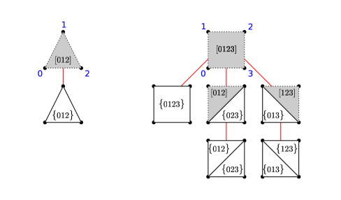
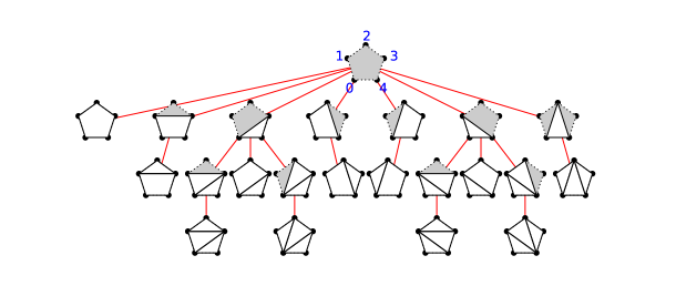
Figure 2. For $n=2,3,4$, the figure depicts the recursion trees obtained by repeatedly applying Equation 7. The top levels of these recursion trees correspond to Equations 9–11.

Proof of the Main Theorem.

This theorem is a generalization of Theorem 1 in [DividedDiffInverse], and the proofs are analogous. We prove the formula by induction on the order $n$ of the divided difference of $y$.

By the above discussion, the formula holds for $n=2,3,4$. For $n\geq 5$, assume the formula holds for all smaller $n$. Consider the recursive formula from Equation 7. For every sequence $\mathbf{i}$ that appears in this equation, the corresponding outer faces have fewer vertices than the full polygon. By the induction hypothesis, we can therefore replace each divided difference $[i_{l}\cdots i_{l+1}]y$ appearing in the product of Equation 7 by an expression involving only divided differences of $g$.

As before, let $\mathcal{P}_{\mathbf{i}}$ denote the set of all partitions of the disjoint union of the outer faces induced by $\mathbf{i}$. Then, by the induction hypothesis, the product in Equation 7 is equal to

$$\sum_{\pi\in\mathcal{P}_{\mathbf{i}}}\prod_{(v_{0},\ldots,v_{r})\in F(\pi)}\{v_{0}\cdots v_{r}\}g.$$

For a given inner face $\mathbf{i}$, the set $\mathcal{P}_{\mathbf{i}}$ can be identified with $\{\pi\in\mathcal{P}(0,\ldots,n):\mathbf{i}\in F(\pi)\}$ by the bijection $F(\pi)\mapsto F(\pi)\cup\{\mathbf{i}\}$. Substituting the above expression into Equation 7 then yields

$$[0\cdots n]y= \sum_{\begin{subarray}{c}\textup{inner faces}\\ \mathbf{i}=(i_{0},\ldots,i_{k})\end{subarray}}\{i_{0}\cdots i_{k}\}g\sum_{\pi\in\mathcal{P}_{\mathbf{i}}}\ \prod_{(v_{0},\ldots,v_{r})\in F(\pi)}\{v_{0}\cdots v_{r}\}g$$

$$= \sum_{\begin{subarray}{c}\textup{inner faces}\\ \mathbf{i}=(i_{0},\ldots,i_{k})\end{subarray}}\ \sum_{\begin{subarray}{c}\pi\in\mathcal{P}(0,\ldots,n)\\ \mathbf{i}\in F(\pi)\end{subarray}}\ \prod_{(v_{0},\ldots,v_{r})\in F(\pi)}\{v_{0}\cdots v_{r}\}g$$

$$= \sum_{\pi\in\mathcal{P}(0,\ldots,n)}\ \prod_{(v_{0},\ldots,v_{r})\in F(\pi)}\{v_{0}\cdots v_{r}\}g.\qed$$

Intuitively, this proof can be expressed in terms of the recursion tree as follows. As remarked in the previous section, Equation 7 states that the expression of any nonleaf vertex is equal to the sum of the expressions of its descendants. By induction, the expression $[01\cdots n]y$ of the root vertex is therefore equal to the sum of the expressions of the leaves, which, by construction, correspond to partitions of the full polygon.

Example 1.

Let us apply Theorem 1 to find a simple expression for divided differences of the function $y(x)=\sqrt{1-x^{2}}$ defined on the interval $(-1,1)$. This function is implicitly defined by the polynomial $g(x,y)=x^{2}+y^{2}-1=0$. For any knots $x_{a},x_{b},x_{c},x_{d}$ satisfying $-1<x_{a}\leq x_{b}\leq x_{c}\leq x_{d}<1$ and corresponding function values $y_{a},y_{b},y_{c},y_{d}$, one finds

$$[x_{a},x_{b};y_{c}]g=x_{a}+x_{b},\qquad[x_{a},x_{b},x_{c};y_{d}]g=1,$$

$$[x_{a};y_{b},y_{c}]g=y_{b}+y_{c},\qquad\ [x_{a};y_{b},y_{c},y_{d}]g=1,$$

and all other divided differences of $g$ of nonzero order are zero. In particular, every divided difference of $g$ of total order at least three is zero, which means that the sum in Equation 15 will only be over triangulations (i.e., partitions in which all faces are triangles). For a polygon with vertices $0,1,\ldots,n$, Exercise 6.19a of [Stanley2] states that the number of such triangulations is given by the Catalan number

$$C(n-1)=\frac{1}{n}{2n-2\choose n-1}.$$

Consider, for a given triangulation $\pi\in\mathcal{P}(0,1,\ldots,n)$, a face $(a,b,c)\in F(\pi)$ from the product in Equation 15. As any divided difference of the form $[x_{a},x_{b};y_{b},y_{c}]g$ is zero for this $g$, Equation 8 expresses $\{abc\}g$ as a sum of at most two terms. There are four cases.

$$\{abc\}g=\left\{\begin{array}[]{ll}\displaystyle\frac{-1}{y_{a}+y_{c}}\left[1+\frac{x_{a}+x_{b}}{y_{a}+y_{b}}\cdot\frac{x_{b}+x_{c}}{y_{b}+y_{c}}\right]&a,b,c~{}\text{consecutive};\\ \displaystyle\frac{1}{y_{a}+y_{c}}\cdot\frac{x_{a}+x_{b}}{y_{a}+y_{b}}&\text{only}~{}a,b~{}\text{consecutive};\\ \displaystyle\frac{1}{y_{a}+y_{c}}\cdot\frac{x_{b}+x_{c}}{y_{b}+y_{c}}&\text{only}~{}b,c~{}\text{consecutive};\\ \displaystyle\frac{-1}{y_{a}+y_{c}}&\text{otherwise}.\end{array}\right.$$

For example, when $n=3$, our convex polygon is a quadrilateral, which admits $C(3-1)=2$ triangulations $\pi_{1}$ and $\pi_{2}$ with sets of faces

$$F(\pi_{1})=\{(0,1,2),(0,2,3)\},\qquad F(\pi_{2})=\{(0,1,3),(1,2,3)\}.$$

One finds

$$[x_{0},x_{1},x_{2},x_{3}]\sqrt{1-x^{2}}=\{012\}g\,\{023\}g+\{013\}g\,\{123\}g=$$

$$\hfill\frac{-1}{(y_{0}+y_{3})(y_{0}+y_{2})}\left[1+\frac{x_{0}+x_{1}}{y_{0}+y_{1}}\cdot\frac{x_{1}+x_{2}}{y_{1}+y_{2}}\right]\cdot\frac{x_{2}+x_{3}}{y_{2}+y_{3}}+$$

$$\hfill\frac{-1}{(y_{0}+y_{3})(y_{1}+y_{3})}\left[1+\frac{x_{1}+x_{2}}{y_{1}+y_{2}}\cdot\frac{x_{2}+x_{3}}{y_{2}+y_{3}}\right]\cdot\frac{x_{0}+x_{1}}{y_{0}+y_{1}}.\ \!\$$

Example 2.

Next we show that Theorem 1 is a generalization of Theorem 1 of [DividedDiffInverse], which gives a similar formula for inverse functions. To see this, we apply Theorem 1 to a function $y$ implicitly defined by a function $g(x,y)=x-h(y)$. Referring to Equation 8, we need to compute $[i_{0}\cdots i_{s};i_{s}\cdots i_{k}]g$ for this choice of $g$ and various indices $i_{0},\ldots,i_{k}$ and $s\in\{0,\ldots,k\}$. Applying the recursive definition of bivariate divided differences, one obtains

$$[i_{0}\cdots i_{s};i_{s}\cdots i_{k}]x\hfill= \left\{\begin{array}[]{ll}x_{i_{0}}&\textup{if}~{}s=0,s=k;\\ 1&\textup{if}~{}s=1,s=k;\\ 0&\textup{otherwise},\end{array}\right.$$

$$[i_{0}\cdots i_{s};i_{s}\cdots i_{k}]h(y)= \left\{\begin{array}[]{ll}[i_{s}\cdots i_{k}]h&\textup{if}~{}s=0;\\ 0&\textup{otherwise}.\end{array}\right.$$

Consider a face $f=(v_{0},\ldots,v_{r})$ of a given partition $\pi\in\mathcal{P}(0,\ldots,n)$ in Equation 15. Since $r\geq 2$, the divided difference $[v_{0}\cdots v_{s};v_{s}\cdots v_{r}]\big{(}x-h(y)\big{)}$ is zero for $s\geq 1$. Using this, Equation 8 expresses $\{v_{0}\cdots v_{r}\}g$ as a single term

$$\{v_{0}\cdots v_{r}\}g= -\frac{[v_{0};v_{0}\cdots v_{r}]g}{[v_{0};v_{0}v_{r}]g}\prod_{\begin{subarray}{c}l=1\\ v_{l}-v_{l-1}=1\end{subarray}}^{r}\left(-\frac{[v_{l-1}v_{l};v_{l}]g}{[v_{l-1};v_{l-1}v_{l}]g}\right)$$

$$= -\frac{[v_{0}\cdots v_{r}]h}{[v_{0}v_{r}]h}\prod_{\begin{subarray}{c}l=1\\ v_{l}-v_{l-1}=1\end{subarray}}^{r}\frac{1}{[v_{l-1}v_{l}]h}.$$

Taking the product over all faces in the partition $\pi$, the denominators of the factors in the above equation correspond to the edges of the partition, while the numerators correspond to the faces of the partition. As there is a minus sign for each face in the partition, we arrive at the formula

(16) $$[01\cdots n]y=\sum_{\pi\in\mathcal{P}(0,\ldots,n)}(-1)^{\#F(\pi)}\frac{\displaystyle\prod_{(v_{0},v_{1},\ldots,v_{r})\in F(\pi)}[v_{0}v_{1}\cdots v_{r}]h}{\displaystyle\prod_{(v_{0},v_{1})\in E(\pi)}[v_{0}v_{1}]h},$$

which appears as Equation 11 in [DividedDiffInverse].

Note that the inverse of the algebraic function $y=\sqrt{1-x^{2}}$ in Example 1 is again an algebraic function. Equation 16 would therefore not have been of much help to find a simple expression for divided differences of $y$. In fact, Example 1 can be thought of as one of the simplest examples for which Theorem 1 improves on Equation 16, as it concerns a polynomial $g$ with bidegree as low as (2,2).

Example 3.

In this example we shall derive a quotient rule for divided differences. That is, we shall find a formula that expresses divided differences of the quotient $y=P(x)/Q(x)$ in terms of divided differences of $P$ and of $Q$. Let $g(x,y)=Q(x)y-P(x)$. Then, in Equation 8,

(17) $$[i_{0}\cdots i_{s};i_{s}\cdots i_{k}]g=\left\{\begin{array}[]{rl}y_{i_{s}}[i_{0}\cdots i_{s}]Q-[i_{0}\cdots i_{s}]P&\textup{if}~{}s=k;\\ \,[i_{0}\cdots i_{s}]Q&\textup{if}~{}s=k-1;\\ 0&\textup{otherwise}.\end{array}\right.$$

In Equation 15, therefore, the only partitions with a nonzero contribution are those whose faces have all their vertices consecutive, except possibly the final one. In particular, the inner face with vertices $0=i_{0}<\cdots<i_{k}=n$ should either be the full polygon, or should have a unique inner edge $(i_{k-1},n)$. By induction, it follows that the partitions with a nonzero contribution to Equation 15 are precisely those for which all inner edges end at $n$. These partitions correspond to subsets $I\subset\{1,2,\ldots,n-2\}$, including the empty set, by associating with any such $I$ the partition with inner edges $\{(i,n)\,:i\,\in I\}$. Equation 15 becomes

(18) $$[0\cdots n]\frac{P}{Q}=\, \{0\cdots n\}g+$$

$$\sum_{r=1}^{n-2}\ \sum_{k=1}^{r}\ \sum_{0=i_{0}<i_{1}<\cdots<i_{k}=r}\{r\cdots n\}g\ \prod_{j=1}^{k}\{i_{j-1}\cdots i_{j}n\}g,$$

where the dots represent consecutive nodes and an empty product is understood to be one. A long but straightforward calculation involving Equations 8, 17, and 18 yields

$$[0\cdots n]\frac{P}{Q}=\, \frac{[0\cdots n]P}{Q_{0}}+$$

$$\sum_{r=1}^{n}\frac{[r\cdots n]P}{Q_{r}}\sum_{k=1}^{r}(-1)^{k}\!\!\sum_{0=i_{0}<i_{1}<\cdots<i_{k}=r}\ \prod_{j=1}^{k}\frac{[i_{j-1}\cdots i_{j}]Q}{Q_{i_{j-1}}},$$

where $Q_{i}:=Q(x_{i})$ for $i=0,\ldots,n$. Alternatively, this equation can be found by applying a univariate chain rule to the composition $x\mapsto Q(x)\mapsto 1/Q(x)$, as described in Section 4 of [DividedDiffChain].

Finally, we note that taking the limit $x_{0},\ldots,x_{n}\to x$ in Equations 6, 8, 12, and 13 yields

$$y^{\prime}(x)= -\frac{g_{10}}{g_{01}},$$

$$y^{\prime\prime}(x)= -\frac{g_{20}}{g_{01}}+2\frac{g_{11}g_{10}}{g_{01}^{2}}-\frac{g_{02}g_{10}^{2}}{g_{01}^{3}},$$

$$y^{\prime\prime\prime}(x)= -\frac{g_{30}}{g_{01}}+3\frac{g_{21}g_{10}}{g_{01}^{2}}+3\frac{g_{20}g_{11}}{g_{01}^{2}}-3\frac{g_{20}g_{10}g_{02}}{g_{01}^{3}}-3\frac{g_{12}g_{10}^{2}}{g_{01}^{3}}$$

$$-6\frac{g_{11}^{2}g_{10}}{g_{01}^{3}}+\frac{g_{10}^{3}g_{03}}{g_{01}^{4}}+9\frac{g_{11}g_{10}^{2}g_{02}}{g_{01}^{4}}-3\frac{g_{10}^{3}g_{02}^{2}}{g_{01}^{5}},$$

where we introduced the shorthand

$$g_{st}:=\frac{\partial^{s+t}g}{\partial x^{s}\partial y^{t}}\big{(}x,y(x)\big{)}.$$

These formulas agree with the examples given in [ComtetFiolet], [Comtet, Page 153] and with a formula stated as Equation 7 in [Wilde].

References

de BoorCarlDivided differencesSurv. Approx. Theory1200546–69 (electronic)Review MathReviews@article{Boor, author = {de Boor, Carl}, title = {Divided differences}, journal = {Surv. Approx. Theory}, volume = {1}, date = {2005}, pages = {46–69 (electronic)}, review = {\MR{2221566 (2006k:41001)}}} FloaterMichael S.LycheTomTwo chain rules for divided differences and faà di bruno’s formulaMath. Comp.762007258867–877 (electronic)ISSN 0025-5718Review MathReviews@article{DividedDiffChain, author = {Floater, Michael S.}, author = {Lyche, Tom}, title = {Two chain rules for divided differences and Fa\`a di Bruno's formula}, journal = {Math. Comp.}, volume = {76}, date = {2007}, number = {258}, pages = {867–877 (electronic)}, issn = {0025-5718}, review = {\MR{2291840 (2008e:65023)}}} FloaterMichael S.LycheTomDivided differences of inverse functions and partitions of a convex polygonMath. Comp.7720082642295–2308ISSN 0025-5718Review MathReviews@article{DividedDiffInverse, author = {Floater, Michael S.}, author = {Lyche, Tom}, title = {Divided differences of inverse functions and partitions of a convex polygon}, journal = {Math. Comp.}, volume = {77}, date = {2008}, number = {264}, pages = {2295–2308}, issn = {0025-5718}, review = {\MR{2429886 (2009e:05027)}}} FloaterMichael S.LycheTomA Chain Rule for Multivariate Divided Differences date=2009 eprint=http://folk.uio.no/michaelf/papers/fdbm.pdf@article{ChainRuleMultivariate, author = {Floater, Michael S.}, author = {Lyche, Tom}, title = {{A Chain Rule for Multivariate Divided Differences} date={2009} eprint={http://folk.uio.no/michaelf/papers/fdbm.pdf}}} WangXinghuaXuAiminOn the divided difference form of faà di bruno’s formula. iiJ. Comput. Math.2520076697–704ISSN 0254-9409Review MathReviews@article{WangXu, author = {Wang, Xinghua}, author = {Xu, Aimin}, title = {On the divided difference form of Fa\`a di Bruno's formula. II}, journal = {J. Comput. Math.}, volume = {25}, date = {2007}, number = {6}, pages = {697–704}, issn = {0254-9409}, review = {\MR{2359959 (2008h:65009)}}} di Bruno,Cavaliere FrancescoFaàNote sur une nouvelle formule de calcul différentielQuarterly J. Pure Appl. Math.11857359–360@article{FaaDiBruno, author = {Fa\`a di Bruno,Cavaliere Francesco}, title = {Note sur une nouvelle formule de calcul diff\'erentiel}, journal = {Quarterly J. Pure Appl. Math.}, volume = {1}, date = {1857}, pages = {359–360}} JohnsonWarren P.The curious history of faà di bruno’s formulaAmer. Math. Monthly10920023217–234ISSN 0002-9890Review MathReviews@article{Johnson-CuriousHistory, author = {Johnson, Warren P.}, title = {The curious history of Fa\`a di Bruno's formula}, journal = {Amer. Math. Monthly}, volume = {109}, date = {2002}, number = {3}, pages = {217–234}, issn = {0002-9890}, review = {\MR{1903577 (2003d:01019)}}} ConstantineG. M.SavitsT. H.A multivariate faà di bruno formula with applicationsTrans. Amer. Math. Soc.34819962503–520ISSN 0002-9947Review MathReviews@article{MultivariateFaaDiBruno, author = {Constantine, G. M.}, author = {Savits, T. H.}, title = {A multivariate Fa\`a di Bruno formula with applications}, journal = {Trans. Amer. Math. Soc.}, volume = {348}, date = {1996}, number = {2}, pages = {503–520}, issn = {0002-9947}, review = {\MR{1325915 (96g:05008)}}} WildeTomImplicit higher derivatives, and a formula of Comtet and Fiolet date=2008-05-17 eprint=http://arxiv.org/abs/0805.2674v1@article{Wilde, author = {Wilde, Tom}, title = {{Implicit higher derivatives, and a formula of Comtet and Fiolet} date={2008-05-17} eprint={http://arxiv.org/abs/0805.2674v1}}} ComtetLouisFioletMichelSur les dérivées successives d’une fonction impliciteFrenchC. R. Acad. Sci. Paris Sér. A2781974249–251Review MathReviews@article{ComtetFiolet, author = {Comtet, Louis}, author = {Fiolet, Michel}, title = {Sur les d\'eriv\'ees successives d'une fonction implicite}, language = {French}, journal = {C. R. Acad. Sci. Paris S\'er. A}, volume = {278}, date = {1974}, pages = {249–251}, review = {\MR{0348055 (50 \#553)}}} ComtetLouisAdvanced combinatoricsRevised and enlarged editionThe art of finite and infinite expansionsD. Reidel Publishing Co.Dordrecht1974xi+343ISBN 90-277-0441-4Review MathReviews@book{Comtet, author = {Comtet, Louis}, title = {Advanced combinatorics}, edition = {Revised and enlarged edition}, note = {The art of finite and infinite expansions}, publisher = {D. Reidel Publishing Co.}, place = {Dordrecht}, date = {1974}, pages = {xi+343}, isbn = {90-277-0441-4}, review = {\MR{0460128 (57 \#124)}}} StanleyRichard P.Enumerative combinatorics. vol. 2Cambridge Studies in Advanced Mathematics62With a foreword by Gian-Carlo Rota and appendix 1 by Sergey FominCambridge University PressCambridge1999xii+581ISBN 0-521-56069-1ISBN 0-521-78987-7Review MathReviews@book{Stanley2, author = {Stanley, Richard P.}, title = {Enumerative combinatorics. Vol. 2}, series = {Cambridge Studies in Advanced Mathematics}, volume = {62}, note = {With a foreword by Gian-Carlo Rota and appendix 1 by Sergey Fomin}, publisher = {Cambridge University Press}, place = {Cambridge}, date = {1999}, pages = {xii+581}, isbn = {0-521-56069-1}, isbn = {0-521-78987-7}, review = {\MR{1676282 (2000k:05026)}}}