Dicke-like quantum phase transition and vacuum entanglement with two coupled atomic ensembles

Abstract

We study the coherent cooperative phenomena of the system composed of two interacting atomic ensembles in the thermodynamic limit. Remarkably, the system exhibits the Dicke-like quantum phase transition and entanglement behavior although the governing Hamiltonian is fundamentally different from the spin-boson Dicke Hamiltonian, offering the opportunity for investigating collective matter-light dynamics with pure matter waves. The model can be realized with two Bose-Einstein condensates or atomic ensembles trapped in two optical cavities coupled to each other. The interaction between the two separate samples is induced by virtual photon exchange.

I INTRODUCTION

Entanglement, arising from nonlocal superposition state of two or more quantum systems, is one of the most striking features of quantum mechanics and plays a key role in the test of local hidden variable theories [1,2]. Over the past two decades entanglement is regarded as a key resource to implement quantum information tasks, such as quantum cryptography [3], computer [4], and teleportation [5]. On the other hand, entanglement is closely related to various collective quantum phenomena and plays a central role in studying quantum many-body systems. Typical examples are entangled ground states used to clarify superconductivity [6] and fractional quantum Hall effect [7]. Ground state entanglement, which is responsible for long-range correlations at zero temperature [8], may shed light upon quantum phase transition [8]. The connection between entanglement and quantum phase transition has been extensively explored in the quantum system made up of N spins 1/2 on a one-dimensional lattice [9-11] or on a simplex [12,13].

Another important example of correlated many-particle systems is the Dicke model [14], which describes the interaction of an ensemble of N two-level systems with a single-mode quantized field. When the atom-field coupling is strong enough such a model exhibits a superradiant quantum phase transition [15-17]. Lambert et al. have investigated the critical behavior of the atom-field entanglement and pairwise entanglement between atoms in the thermodynamics limit [18]. The Dicke model has also been a fertile ground for implementation of quantum information as atomic ensembles with long-lived electronic states are ideal for storing and processing local quantum information via interaction with light fields. High-fidelity quantum operations and entanglement may be achieved beyond the strong coupling between a single atom and a single photon due to the collective enhancement of interaction with the field mode [19].

The Dicke quantum phase transition occurs under the condition that the coupling strength is on the order of the energy separation between two involved levels and thus the counter-rotating terms significantly affect the dynamics, which is difficult to achieve in typical cavity QED systems since the atomic transition frequencies usually exeed the atom-cavity coupling strength by many orders of magnitude. Dimer et al. have propsed an effective Dicke model based on balanced Raman transitions between two ground atomic states of an atomic ensemble induced by a cavity mode and a pair of laser fields [20], which significantly lowers the energy difference between the two involved levels. It has been shown that the Dicke model can also been realized in a laser-driven Bose-Einstein condensate coupled to an optical cavity and the onset of self-organization corresponds to the Dicke quantum phase transition [21-23]. However, these systems are subject to cavity loss, which would significantly alter the coherent dynamics of the Hamiltonian and deteriorate the matter-light entanglement. Though the superradiant quantum phase transition has been observed in Ref. [22], the ground state entanglement has not been verified.

In this paper we investigate the collective dynamics of the system that consists of two coupled atomic ensembles and find two main results. Firstly, we show that the coupled spin system can display the quantum phase transition and vacuum entanglement properties of the physically distinct spin-boson Dicke model in the thermodynamic limit, providing an access to the intriguing critical entanglement of the Dicke model without involving the dynamics of the quantized field. Secondly, as an example for the physical implementation of this model we demonstrate that two Bose-Einstein condensates (BECs) or atomic ensembles trapped in two coupled optical cavities can form the effective spin Hamiltonian. With the assistance of suitable chosen external fields, the virtual excitation of the cavity modes mediates effective coupling between the two spin ensembles. Besides fundamental interest, the system offers the possibility to produce two-mode squeezed vacuum states between two spatially separated macroscopic systems, which are of crucial importance for quantum communication [24] and nonlocality test [25] with continuous variables. Such states are also useful for exploring the boundary between quantum and classical worlds and understanding the decoherence effect in quantum information.

The paper is organized as follows. In Sec.2, we study the Hamiltonian dynamics of two coupled atomic ensembles in the thermodynamic limit, and show that the system can exhibit the quantum phase transition and critical entanglement behavior of the Dicke model. In Sec.3, we propose an experimental realization of the system by coupling the motional degrees of freedom of two BECs trapped in two coupled optical cavities. The model can also be realized in the electronic degrees of freedom of two atomic ensembles via virtual photon exchange. A summary appears in Sec.4.

II QUANTUM PHASE TRANSITION AND VACUUM ENTANGLEMENT

Let us start by considering the system involving two coupled atomic ensembles, with the $i$th ($i=1$, $2$) ensemble consisting of $N_{i}$ two-level atoms of energy splitting $\omega_{i}$. The Hamiltonian of the system is given by

$$H=\omega_{1}J_{1,z}+\omega_{2}J_{2,z}+\frac{\lambda}{\sqrt{N_{1}N_{2}}}(J_{1}^{+}+J_{1}^{-})(J_{2}^{+}+J_{2}^{-}),$$ (1)

where {$J_{i,z},J_{i}^{\pm}\}$ are collective atomic operators for the $i$th ensemble, satisfying the angular momentum commutation relations $[J_{i}^{+},J_{i}^{-}]=2J_{i,z}$ and $[J_{i}^{\pm},J_{i,z}]=\mp J_{i}^{\pm}$. The Hamiltonian commutes with the partity operator $e^{i\pi(J_{1,z}+J_{2,z})}$. Using the Holstein-Primakoff representation, we express the operators {$J_{i,z},J_{i}^{\pm}\}$ in terms of the annihilation and creation operators $b_{i}$ and $b_{i}^{\dagger}$ of a bosonic mode via $J_{i}^{+}=b_{i}^{\dagger}\sqrt{N_{i}-b_{i}^{\dagger}b_{i}}$, $J_{i}^{-}=\sqrt{N_{i}-b_{i}^{\dagger}b_{i}}b_{i}$, and $J_{i,z}=b_{i}^{\dagger}b_{i}-N_{i}/2$. Then we obtain the two-mode bosonic Hamiltonian

$$H = \omega_{1}b_{1}^{\dagger}b_{1}+\omega_{2}b_{2}^{\dagger}b_{2}$$ (4)

$$+\frac{\lambda}{\sqrt{N_{1}N_{2}}}\left(b_{1}^{\dagger}\sqrt{N_{1}-b_{1}^{\dagger}b_{1}}+\sqrt{N_{1}-b_{1}^{\dagger}b_{1}}b_{1}\right)$$

$$\times\left(b_{2}^{\dagger}\sqrt{N_{2}-b_{2}^{\dagger}b_{2}}+\sqrt{N_{2}-b_{2}^{\dagger}b_{2}}b_{2}\right).$$

Perform the transformation $D_{1}^{+}(\alpha)D_{2}^{+}\left(\beta\right)HD_{1}(\alpha)D_{2}\left(\beta\right)$, where $D_{1}(\alpha)=e^{\alpha b_{i}^{\dagger}-\alpha^{*}b_{i}}$ and $D_{2}(\beta)=e^{\beta b_{i}^{\dagger}-\beta^{*}b_{i}}$ are displacement operators. In the thermodynamic limit $N_{i}\rightarrow\infty$ we can approximate the square root terms up to $1/N_{i}$. The resulting Hamiltonian is expanded up to the second-order in the boson operators.

In order for the coefficients of the linear terms in the displaced Hamiltonian to be zero, the displacement amounts $\alpha$ and $\beta$ should satisfy

$$\omega_{1}\alpha+2\lambda\beta\frac{N_{1}-2\alpha^{2}}{\sqrt{N_{1}N_{2}}}\sqrt{\frac{N_{2}-\beta^{2}}{N_{1}-\alpha^{2}}} = 0,$$ (5)

$$\omega_{2}\beta+2\lambda\alpha\frac{N_{2}-2\beta^{2}}{\sqrt{N_{1}N_{2}}}\sqrt{\frac{N_{1}-\alpha^{2}}{N_{2}-\beta^{2}}} = 0.$$ (6)

Under the critical point $\lambda_{c}=\sqrt{\omega_{1}\omega_{2}}/2$, the solution is $\alpha=\beta=0$, which corresponds to the normal phase. In this case the effective Hamiltonian $H^{(1)}=\omega_{1}b_{1}^{\dagger}b_{1}+\omega_{2}b_{2}^{\dagger}b_{2}+\lambda(b_{1}^{\dagger}+b_{1})(b_{2}^{\dagger}+b_{2})$ is mathematically equivalent to the spin-boson Dicke Hamiltonian in the normal phase [15]. The ground state in this phase is a two-mode squeezed vacuum state, which has a definite partiy and is incoherent, i.e., $\left\langle(J_{i}^{+}+J_{i}^{-})\right\rangle=0$.

Above the critical point, there exist two physically sensible solutions {$\alpha=\sqrt{N_{1}}\alpha_{0},\beta=-\sqrt{N_{2}}\beta_{0}$} and {$\alpha=-\sqrt{N_{1}}\alpha_{0}$, $\beta=\sqrt{N_{2}}\beta_{0}$}, where $\alpha_{0}=\{\frac{1}{2}[1-\sqrt{\frac{4\lambda^{2}\omega_{1}^{2}+r(\omega_{1}\omega_{2})^{2}}{4\lambda^{2}\omega_{1}^{2}+16r\lambda^{4}}}]\}^{1/2}$, $\beta_{0}=\{\frac{1}{2}[1-\sqrt{\frac{4r\lambda^{2}\omega_{2}^{2}+(\omega_{1}\omega_{2})^{2}}{4r\lambda^{2}\omega_{2}^{2}+16\lambda^{4}}}]\}^{1/2}$, and $r=N_{2}/N_{1}$. The corresponding effective Hamiltonian is

$$H^{(2)} = \frac{K_{1}+K_{2}}{2}b_{1}^{\dagger}b_{1}+\frac{K_{1}-K_{2}}{4}(b_{1}^{\dagger 2}+b_{1}^{2})$$ (9)

$$+\frac{K_{3}+K_{4}}{2}b_{2}^{\dagger}b_{2}+\frac{K_{3}-K_{4}}{4}(b_{2}^{\dagger 2}+b_{2}^{2})$$

$$+K_{5}(b_{1}^{\dagger}+b_{1})(b_{2}^{\dagger}+b_{2}),$$

where

$$K_{1} = \omega_{1}-\frac{2\alpha_{0}\beta_{0}(3-2\alpha_{0}^{2})\sqrt{r(1-\beta_{0}^{2})}\lambda}{(1-\alpha_{0}^{2})^{3/2}},$$ (10)

$$K_{2} = \omega_{1}-2\alpha_{0}\beta_{0}\lambda\sqrt{\frac{r(1-\beta_{0}^{2})}{1-\alpha_{0}^{2}}},$$

$$K_{3} = \omega_{2}-\frac{2\alpha_{0}\beta_{0}(3-2\beta_{0}^{2})\sqrt{(1-\alpha_{0}^{2})/r}\lambda}{(1-\beta_{0}^{2})^{3/2}},$$

$$K_{4} = \omega_{2}-2\alpha_{0}\beta_{0}\lambda\sqrt{\frac{1-\alpha_{0}^{2}}{r(1-\beta_{0}^{2})}},$$ (11)

$$K_{5} = \frac{(1-2\alpha_{0}^{2})(1-2\beta_{0}^{2})\lambda}{(1-\alpha_{0}^{2})^{1/2}(1-\beta_{0}^{2})^{1/2}}.$$ (12)

The Hamiltonian $H^{(2)}$ is diagonal in terms of two normal bosonic modes with the frequencies

$$\omega_{\pm}^{2} = \frac{K_{1}K_{2}+K_{3}K_{4}}{2}$$ (14)

$$\pm\left[\frac{(K_{1}K_{2}-K_{3}K_{4})^{2}}{4}+4K_{2}K_{4}K_{5}^{2}\right]^{1/2}.$$

In the regime near the critical point, the energy gap to the first excited state vanishes as $\omega_{-}\propto\left|\lambda-\lambda_{c}\right|^{1/2}$. Above the threshold, in addition to two-mode squeezing both modes exhibit single-mode squeezing since the coefficient of $b_{i}^{\dagger 2}+b_{i}^{2}$ does not vanish for each mode. However, the single-mode squeezing does not affect the entanglement between the two collective atomic modes. Below the threshold, the single-mode squeezing vanishes and thus the threshold is not affected.

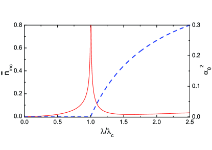
Figure 1: (Color online) The mean excitation number as a function of $\lambda/\lambda_{c}$. The solid line represents the incoherent excitation number due to the squeezing, while the dashed line represents the scaled coherent excitation number, given by the coherent excitation number devided by $N$. The parameters are $\omega_{1}=\omega_{2}=\omega$, $\lambda_{c}=\omega/2$, and $N_{1}=N_{2}=N$.

Above the threshould, there are two degenerate ground states, which corresponds to the breaking of the parity symmetry with the atomic polarizations $\left\langle(J_{1}^{+}+J_{1}^{-})\right\rangle=2\alpha\sqrt{N_{1}-\alpha^{2}}$ and $\left\langle(J_{2}^{+}+J_{2}^{-})\right\rangle=2\beta\sqrt{N_{2}-\beta^{2}}$ acquiring macroscopic populations. In this phase both the coherent excitation and squeezing contribute to the excited atomic numbers. This is analogous to the superradiant phase of the spin-boson Dicke model with the field mode replaced by another atomic mode. The excitation number of each ensemble as a function of $\lambda/\lambda_{c}$ is ploted in Fig. 1. The solid line represents the incoherent excitation number due to squeezing, while the dashed line represents the scaled coherent excitation number. Near the critical point the incoherent excitation number of each atomic ensemble due to squeezing is $\stackrel{{\scriptstyle-}}{{n}}_{inc}\infty\left|\lambda-\lambda_{c}\right|^{-1/4}$, which diverges with the same exponent $1/4$ as the correlation length $\xi=\omega_{-}^{-1/2}$. The entanglement between the two atomic ensembles can be determined by the von Neumann entropy $S=-$tr$\rho\log_{2}\rho$, where $\rho$ is the reduced density operator of one atomic ensemble. In the superexcitation phase, this entropy is given by

$$S=(k+1/2)\log_{2}(k+1/2)-(k-1/2)\log_{2}(k-1/2)+1,$$ (15)

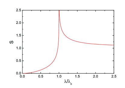
Figure 2: (Color online) The entanglement entropy between the two atomic ensembles as a function of $\lambda/\lambda_{c}$. The parameters are $\omega_{1}=\omega_{2}=\omega$, $\lambda_{c}=\omega/2$, and $N_{1}=N_{2}=N$.

where $k=\frac{1}{2}\left[1+\frac{\sin^{2}2\theta}{4}(\sqrt{\omega_{+}/\omega_{-}}-\sqrt{\omega_{-}/\omega_{+}})^{2}\right]^{1/2}$ and $\theta=\frac{1}{2}\arctan[2K_{5}\sqrt{K_{2}K_{4}}/(K_{1}K_{2}-K_{3}K_{4})]$. The entanglement as a function of $\lambda/\lambda_{c}$ can be seen in Fig. 2. At the critical point the entanglement diverges logarithmically also with the exponent $1/4$ as $S\infty\log_{2}\left|\lambda-\lambda_{c}\right|^{-1/4}$, which is analogous to the critical behavior of the atom-field entanglement in the Dicke model [18]. In the above we have assumed that $\lambda>0$. It should be noted that the system exhibits the same critical behavior and entanglement for $\lambda<0$.

III PHYSICAL REALIZATION

We note that the Hamiltonian (1) can be realized in the quantum motions of two BECs or atomic ensembles trapped in two coupled single-mode cavities along the $x$-axis. The resonant coupling between the two cavity modes is given by the interaction Hamiltonian $H_{c}=\nu(a_{1}^{\dagger}a_{2}+a_{1}a_{2}^{+})$, where $a_{i}^{\dagger}$ and $a_{i}$ are the creation and annihilation operators for the $i$th cavity mode, and $\nu$ is the intercavity hopping strength. Such a coupling can be mediated by overlap of their evanescent fields or by an optical fiber [26].

We first consider the cavity-BEC system. Suppose that the $i$th BEC is composed of $N_{i}$ two-level atoms, each of which is coupled to the $i$th cavity mode with the maximum coupling strength $g_{i}$ and driven by a pump laser field along the $y$-axis with the maximum Rabi frequency $\Omega_{i}$. The pump frequency $\omega_{p}$, close to the cavity mode frequency $\omega_{c}$, is highly detuned from the atomic transition frequency $\omega_{a}$. Then the atomic excited level can be adiabatically eliminated and the atoms coherently scatter light between the pump field and the cavity mode, which induce two balanced Raman channels between the atomic zero-momentum state and the symmetric superposition of states with the momentum of a photon, $\hbar k$, along the $x$ and $y$ directions. Hence each atomic field can be described in a Hilbert space spanned by two Fourier-modes $c_{0,i}$ and $c_{1,i}$, with $c_{0,i}^{\dagger}c_{0,i}+c_{1,i}^{\dagger}c_{1,i}=N_{i}$ being a constant of motion [21,22]. The coupling between the two modes can be described by the angular momentum operators: $J_{i}^{+}=c_{1,i}^{\dagger}c_{0,i}$, $J_{i}^{-}=c_{0,i}^{\dagger}c_{1,i}$, and $J_{i,z}=\frac{1}{2}(c_{1,i}^{\dagger}c_{1,i}-c_{0,i}^{\dagger}c_{0,i})$. In the frame rotating with the pump field frequency $\omega_{p}$ the Hamiltonian for the $i$th BEC-cavity system is

$$H_{i}=\delta_{c,i}a_{i}^{\dagger}a_{i}+\omega_{0}J_{i,z}-\frac{\eta_{i}}{2}(a_{1}+a_{1}^{\dagger})(J_{i}^{+}+J_{i}^{-})-u_{i}a_{i}^{\dagger}a_{i}c_{1,i}^{\dagger}c_{1,i},$$ (16)

$\delta_{c,i}=\omega_{c}-\omega_{p}-N_{i}g_{i}^{2}/(2\Delta_{a})$, $\omega_{0}=\hbar k^{2}/m$, $\eta_{i}=g_{i}\Omega_{i}/\Delta_{a}$, $u_{i}=3g_{i}^{2}/(4\Delta_{a})$, and $\Delta_{a}=\omega_{a}-\omega_{c}$. Under the condition $N_{1}=N_{2}$ and $g_{1}=g_{2}$ we can choose the pump frequency appropriately so that $\delta_{c,i}=0$. Introducing the new bosonic modes $d_{1,2}=\frac{1}{\sqrt{2}}(a_{1}\pm a_{2})$, we can rewrite the Hamiltonian of the total system as

$$H_{t} = \nu d_{1}^{\dagger}d_{1}-\nu d_{2}^{\dagger}d_{2}+\omega_{0}J_{1,z}+\omega_{0}J_{2,z}$$ (18)

$$\ -\frac{\eta_{1}}{2\sqrt{2}}(d_{1}+d_{1}^{\dagger}+d_{2}+d_{2}^{\dagger})(J_{1}^{+}+J_{1}^{-})$$

$$\ -\frac{\eta_{2}}{2\sqrt{2}}(d_{1}+d_{1}^{\dagger}-d_{2}-d_{2}^{\dagger})(J_{2}^{+}+J_{2}^{-})$$

$$\ \ \ \ \ -\frac{u_{1}}{2}(d_{1}^{\dagger}d_{1}+d_{2}^{\dagger}d_{2}+d_{1}^{\dagger}d_{2}+d_{2}^{\dagger}d_{1})c_{1,1}^{\dagger}c_{1,1}$$

$$\ \ \ \ \ -\frac{u_{2}}{2}(d_{1}^{\dagger}d_{1}+d_{2}^{\dagger}d_{2}-d_{1}^{\dagger}d_{2}-d_{2}^{\dagger}d_{1})c_{1,2}^{\dagger}c_{1,2}.$$

Under the condition $\nu\gg\sqrt{N_{i}}\eta_{i}$, $\omega_{0}$, $\stackrel{{\scriptstyle-}}{{n}}_{i}u_{i}$, $\delta_{c,i}$ , where $\stackrel{{\scriptstyle-}}{{n}}_{i}$ being the mean motional excitation number in the ith BEC, one can adiabatically eliminate the field modes to obtain the coupling between the two condensates. So the effective Hamiltonian is given by

$$H_{e} = \nu d_{1}^{\dagger}d_{1}-\nu d_{2}^{\dagger}d_{2}+\omega_{0}J_{1,z}+\omega_{0}J_{2,z}$$ (22)

$$+\frac{\lambda}{\sqrt{N_{1}N_{2}}}(J_{1}^{+}+J_{1}^{-})(J_{2}^{+}+J_{2}^{-})$$

$$\ \ \ -\frac{1}{2}(u_{1}d_{1}^{\dagger}d_{1}+u_{2}d_{2}^{\dagger}d_{2})(c_{1,1}^{\dagger}c_{1,1}+c_{1,2}^{\dagger}c_{1,2})$$

$$\ +\frac{1}{4\nu}(d_{1}^{\dagger}d_{1}-d_{2}^{\dagger}d_{2})(u_{1}c_{1,1}^{\dagger}c_{1,1}-u_{2}c_{1,2}^{\dagger}c_{1,2})^{2},$$

where $\lambda=-\sqrt{N_{1}N_{2}}\eta_{1}\eta_{2}/(2\nu)$. The Hamiltonian describes a four-photon process which is induced by virtual excitation of the atomic electronic states and field modes. We note that there is no coupling between atoms belonging to the same ensembles since the detunings of the two nonlocal field modes $d_{1}$ and $d_{2}$ are opposite, which leads to opposite contributions to the coupling. On the other hand, these two nonlocal modes equally contribute to the couplings between atoms belonging to different ensembles because the product of the two Raman transition coefficients associated with mode $d_{1}$ is also opposite to that associated with $d_{2}$. When the two cavity modes are both initially in the vacuum state, the two bosonic modes $d_{1}$ and $d_{2}$ will approximately remain in the vacuum state during the evolution since their frequencies are highly detuned from the pump frequency due to the strong coupling between the two cavities. In this case the effective Hamiltonian reduces to Eq. (1), with the effective coupling strength $\lambda$ being controllable by the Rabi frequencies or detunings of the pump fields. The quantum phase transition corresponds to the simultaneous self-organization of the two condensates. In a realistic experiment, the system is a driven and damping one, which will realize a steady state governed by energy flow from the pump fields into the cavity fields, rather than a true ground state of the Hamiltonian, similar to that studied in Ref. [22].

The Hamiltonian (1) can also be realized in the electronic degrees of freedom of two atomic ensembles trapped in two coupled cavities. The cavity mode, together with two external fields, can induce balanced off-resonant Raman transitions between two ground states of each atomic ensemble [20,27]. With appropriate choice of the parameters of the external fields, the field modes can be adiabatically eleminated and the two atomic ensembles are coupled via virtual photon exchange. Due to the stability of the atomic ground states the vacuum entanglement between the two atomic ensembles should have a long coherence lifetime and can be readily transferred to light fields.

IV SUMMARY

In conclusion, we have investigated theoretically the ground state properties of the model involving two coupled spin ensembles in the thermal limit, showing that the model displays the quantum phase transition and vacuum entanglement described by the Dicke model despite the fundamental disctinction between these two models. The model can be realized in the motions of two BECs or in the internal states of two atomic ensembles in two coupled cavities. The coupling strength between the two spin ensembles can be tuned via the parameters of external fields, making the system a promising simulator for this model. The entanglement within each atomic ensemble and its connection with the quantum phase transition will be further investigated. Another interesting problem is how the interaction between atoms belonging to the same ensembles affects the critical behavior and entanglement.

This work was supported by the National Natural Science Foundation of China under Grant No. 10974028, the Doctoral Foundation of the Ministry of Education of China under Grant No. 20093514110009, and the Natural Science Foundation of Fujian Province under Grant No. 2009J06002.

References

- (1) J. S. Bell, Physics 1, 195 (1965).
- (2) D. M. Greenberger, M. A. Horne, and A. Zeilinger, in Bell,s Theorem, Quantum Theory, and Conceptions of the Universe, edited by M. Kafatos (Kluwer, Dordrecht, 1989); D. M. Greenberger, M. A. Horne, A. Shimony, and A. Zeilinger, Am. J. Phys. 58, 1131 (1990).
- (3) A. K. Ekert, Phys. Rev. Lett. 67, 661 (1991).
- (4) D. Deutsch and R. Jozsa, Pro. R. Soc. London A 439, 553 (1992).
- (5) C. H. Bennett, G. Brassard, C. Crepeau, R. Jozsa. A. Peres and W. Wootters, Phys. Rev. Lett. 70, 1895 (1993).
- (6) J. Bardeen, L. N. Cooper, and J. R. Schrieffer, Phys. Rev. 106, 162 (1957); 108, 1175 (1957).
- (7) R. B. Laughlin, Phys. Rev. Lett. 50, 1395 (1983).
- (8) T. J. Osborne and M. A. Nielsen, Quant. Inf. Proc. 1, 45 (2002).
- (9) T. J. Osborne and M. A. Nielsen, Phys. Rev. A 66, 032110 (2002).
- (10) A. Osterloh, L. Amico, G. Falci, and R. Fazio, Nature 416, 608 (2002).
- (11) G. Vidal, J.I. Latorre, E. Rico, and A. Kitaev, Phys. Rev. Lett. 90, 227902 (2003).
- (12) J. Vidal, G. Palacios, and R. Mosseri, Phys. Rev. A 69, 022107 (2004).
- (13) S. Morrison and A. S. Parkins, Phys. Rev. Lett. 100, 040403 (2008).
- (14) R. H. Dicke, Phys. Rev. 93, 99 (1954).
- (15) K. Hepp and E. H. Liep, Ann. Phys. (N.Y.) 76, 360 (1973).
- (16) K. Hepp and E. H. Liep, Phys. Rev. A 8, 2517 (1973).
- (17) Y.K. Wang and F.T.Hioe, Phys. Rev. A 7, 831 (1973).
- (18) N. Lambert, C. Emary, and T. Brandes, Phys. Rev. Lett. 92, 073602 (2004); Phys. Rev. A 71, 053804 (2005).
- (19) K. Hammerer, A. Srensen, and E. S. Polzik, Rev. Mod. Phys. 82, 1014 (2010).
- (20) F. Dimer, B. Estienne, A. S. Parkins, and H. J. Carmichael, Phys. Rev. A 75, 013804 (2007).
- (21) D.Nagy, G. Konya, G. Szirmai, and P. Domokos, Phys. Rev. Lett. 104, 130401 (2010).
- (22) K. Baumann, C. Guerlin, F. Brennecke, and T. Esslinger, Nature 464, 1301 (2010).
- (23) J. Keeling, M. J. Bhaseen, and B. D. Simons, Phys. Rev. Lett. 105, 043001 (2010).
- (24) S. L. Braunstein and P. van Loock, Rev. Mod. Phys. 77, 513 (2005).
- (25) H. Jeong, W. Son, M. S. Kim, D. Ahn, and C. Brukner, Phys. Rev. A 67, 012106 (2003).
- (26) M. J. Hartmann, F. G. S. L. Brandão, and M. B. Plenio, Phys. Rev. Lett. 99, 160501 (2007); Laser & Photon. Rev. 2, 527 (2008).
- (27) S. Morrison and A. S. Parkins, Phys. Rev. Lett. 100, 040403 (2008).