Spectral Properties and the Effect on Redshift Cut-off of Compact AGNs from the AT20G Survey

Abstract

We use high angular resolution data, measured from visibility of sources at the longest baseline of 4500 m of the Australia Telescope Compact Array (ATCA), for the Australia Telescope 20 GHz (AT20G) survey to obtain angular size information for $>$ 94% of AT20G sources. We confirm the previous AT20G result that due to the high survey frequency of 20 GHz, the source population is strongly dominated by compact sources (79%). At 0.15 arcseconds angular resolution limit, we show a very strong correlation between the compact and extended sources with flat and steep-spectrum sources respectively. Thus, we provide a firm physical basis for the traditional spectral classification into flat and steep-spectrum sources to separate compact and extended sources. We find the cut-off of -0.46 to be optimum for spectral indices between 1 and 5 GHz and, hence, recommend the continued use of -0.5 for future studies.

We study the effect of spectral curvature on redshift cut-off of compact AGNs using recently published redshift data. Using spectral indices at different frequencies, we correct for the redshift effect and produce restframe frequency spectra for compact sources for redshift up to $\sim$ 5. We show that the flat spectra of most compact sources start to steepen at $\sim$ 30 GHz. At higher frequencies, the spectra of both populations are steep so the use of spectral index does not separate the compact and extended source populations as well as in lower frequencies. We find that due to the spectral steepening, surveys of compact sources at higher frequencies ($>$ 5 GHz) will have redshift cut-off due to spectral curvature but at lower frequencies, the surveys are not significantly affected by spectral curvature, thus, the evidence for a strong redshift cut-off in AGNs found in lower frequency surveys is a real cut-off and not a result of K-correction.

1 Introduction

Strong evolution of the number density of Active Galactic Nuclei (AGNs) with redshift has been discussed in many papers. Studies done in optical, X-ray and radio frequencies have identified a “quasar epoch”, where the number density rises sharply as a function of redshift from z = 0 to redshift of about 2.5 to 3. The space density has been shown to decline beyond the redshift of 3 in flat-spectrum radio sources (eg. Peacock 1985; Dunlop & Peacock 1990; Shaver et al. 1996; Wall et al. 2005), in X-ray selected quasars (Hasinger et al., 2005) and optically selected quasars (Schmidt et al., 1991; Vigotti et al., 2003). The details of whether such an evolution is purely due to space density evolution or due to luminosity evolution is yet to be resolved. Similarly, the decline in the number density in steep-spectrum radio sources has also been discussed in the literature (eg. Dunlop & Peacock (1990); Jarvis et al. (2001)) and has been studied in detail by Rigby et al. (2011).

The decline in the number density of QSO population beyond redshift $\sim$ 3 has been termed “redshift cut-off” and has been explored in some detail by many authors. Some explanations offered suggest luminosity dependent space density evolution (Dunlop & Peacock, 1990) while others suggest luminosity evolution (e.g. Boyle, Shanks, & Peterson, 1988). The rate of decline in the number density has also been discussed in detail. For example, Dunlop & Peacock (1990) and Vigotti et al. (2003) suggest a slow decline while Shaver et al. (1996) and Wall et al. (2005) find a rapid decline in the number density of flat-spectrum radio quasars at high redshift, comparable to results from X-ray and optical work. However, Jarvis & Rawlings (2000) have argued that spectral curvature causes the observable volume at high redshift universe to be too small to find any luminous flat-spectrum sources, removing the evidence for the rapid decline in number density at high redshift suggested by Shaver et al. (1996). The spectral curvature of sources at different redshifts gives the impression of redshift cut-off by causing the sources to fall outside of selection criteria either by making the flux density fall under the selection limit or the spectral index to fall outside the selection limit, in populations selected based on their spectra (eg. flat-spectrum population). Wall et al. (2005) have found that the use of non-contemporaneous flux density data can cause the effect of steep spectral curvature similar to that seen by Jarvis & Rawlings (2000) (see also de Zotti et al. (2010)).

The abundance of quasars at redshifts 2.5 - 3 has implications for the epoch of formation of the first structures in the universe, which has important consequences for the formation and evolution of massive galaxies. This epoch also has importance in determining whether AGNs can be significant sources of reionization of the universe.

Radio frequency studies of the redshift cut-off have the advantage of being free from dust obscuration. Such studies have been done in the past with populations of flat-spectrum sources, selected from low frequency ($\leq$ 5 GHz) source catalogues. Flat-spectrum sources have traditionally been associated with compact sources (Wall, 1977) with the spectral transition placed variably around $-0.4$ (eg. Shaver 1995; Wall et al. 2005), $-0.5$ (eg. Peacock 1985; Saikia et al. 2001; Browne et al. 2003) or $-0.6$ (eg. De Breuck et al. 2000). In this paper, we follow the convention of $S_{\nu}\propto\nu^{\alpha}$ and use -0.5 as the flat-spectrum cut-off. The flat-spectrum arises from the cumulative effect of multiple, very compact, self absorbed components peaking at different frequencies. Thus, compact AGNs are considered to have a very flat-spectrum, often spanning decades of frequencies.

The Australia Telescope 20 GHz (AT20G) survey (Murphy et al., 2010) is a complete sample of radio sources and is dominated by compact QSOs, due to its high frequency selection (Sadler et al., 2006). These sources have spectra measured at one to three different frequencies (20 GHz, 8.6 GHz and 4.8 GHz) and have counterparts at one to two low frequencies ($\sim$ 1 GHz) . The three high frequencies were measured near simultaneously as part of the survey to remove any effects of variability. Sadler et al. (2006) find the median variability index at 20 GHz to be 6.9 per cent with 5 per cent of sources varying by $>$ 30 per cent in flux density on a 1-2 year time-scale. The AT20G sources also have an angular size measurement at sub arcsec resolution which cleanly separates the compact AGNs from their jets and extended radio-lobes. In this paper, we demonstrate the strong correlation between compact sources and flat-spectrum sources providing a firm physical basis for the use of spectral index for such a separation. We then look at the radio spectrum of these compact sources to investigate the effect of redshift cut-off.

In section 2, we outline the source sample used for this investigation. In section 3, we explain the use of visibility to obtain an angular size measurement. Section 4 discusses the measurement of spectra of compact sources. Section 5 discusses the properties of such compact sources. In section 6 we investigate the effect of spectral curvature and its effect on the redshift cut-off of QSOs. Section 7 is the summary of this work. $\Lambda$CDM cosmology with $H_{0}=71~{}\rm{kms^{-1}Mpc^{-1}}$, $\Omega_{m}=0.27$ and $\Omega_{\Lambda}=0.73$ (Larson et al., 2011) has been used for this paper.

2 The AT20G sample

The AT20G is a blind extragalactic survey carried out at a high frequency of 20 GHz for all declinations of the southern sky using the Australia Telescope Compact Array (ATCA). It covers a total area of 20, 086 deg². It has a galactic latitude cut-off $|b|=1.5$ degrees. The survey has a total of 5890 sources above the flux density limit of 40 mJy at 20 GHz. The AT20G is the largest blind survey done at such a high radio frequency. Most sources south of the declination of -15 degrees have near-simultaneous follow-up observations within a month at 4.8 and 8.6 GHz (Murphy et al., 2010). The sources not observed at 4.8 and 8.6 GHz were a result of scheduling logistics and can not introduce any spectral bias. The cross-match of AT20G sources against the 1.4 GHz NVSS (Condon et al., 1998) catalogue for sources north of $\delta=-40$ degrees and 0.843 GHz SUMSS (Mauch et al., 2003) catalogue for sources south of $\delta=-30$ degrees provides between one to two spectral points near 1 GHz resulting in flux densities at two to five frequencies for the sample. Although the lower frequency points are not simultaneous, there is relatively little variability at these frequencies. Despite the galactic cut-off, the AT20G catalogue still contains a small number of galactic thermal sources which are extended sources of optically thin (flat-spectrum) free-free emission. These high latitude sources are easily seen in H$\alpha$ surveys and have been identified and removed from the main population for this analysis of the extragalactic sources.

Interferometric visibilities on long spacings (henceforth: 6km visibility) for $>94\%$ of the AT20G sources have been measured (see section 3). 3403 AT20G sources have four or more spectral points between 1 and 20 GHz as well as 6km visibility. Optical identifications for 3873 AT20G sources have been made and redshifts of 1460 sources have been compiled (Mahony et al., 2011). This work makes use of the subpopulation of 838 sources with measured redshift, 6km visibility and flux densities measured at four to five frequencies. Table 1 provides a summary of the different subpopulations.

Table 1: Number of AT20G sources with follow-ups, cross-matches with low frequency catalogues and optical counterparts.

Population	Number
Total AT20G	5890
6km visibility measured	5542
$AT20G^{1}$	3795
$AT20G^{1}$ + 6km visibility + NVSS/SUMSS	3403
AT20G + Optical ID	3873
AT20G + Optical ID + Redshift	1460
AT20G + Optical ID + Redshift +
6km visibility + NVSS/SUMSS	1377
$AT20G^{1}$ + Optical ID + Redshift +
6km visibility + NVSS/SUMSS	838

$AT20G^{1}$ is the subpopulation of AT20G with 8.6 and 4.8 GHz follow-up. Sources with $\delta>-15\degr$ do not have 8.6 and 4.8 GHz follow-up.

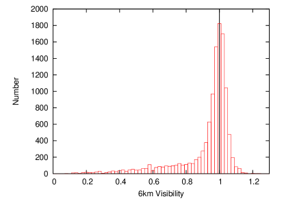
Figure 1: The distribution of all 6km visibilities in the AT20G. Unresolved sources have a visibility of 1 marked by the solid vertical line.

3 The measurement of source size

The AT20G follow-up was done with the hybrid configurations of the ATCA, with five antennae in a compact configuration and the sixth antenna (called the 6km antenna in this paper) at a baseline of $\sim 4500$m from the location of the compact configuration. This allowed us to calculate a visibility amplitude for over 94% of AT20G sources (Table 1). The remaining sources do not have their 6km visibility due to inclement weather during observation or unavailability of the 6km antenna due to maintenance. Thus, the sources with the visibility data are free from any bias.

We calculate the 6km visibility from the ratio of the scalar average of the five long baseline amplitudes to the scalar average of the 10 short baseline amplitudes for the AT20G sources at 20 GHz (Chhetri et al. in prep). Although, the AT20G follow-up observations were done in a hybrid mode, the ATCA when used with its 6km antenna is essentially a linear array. So, the 6km visibility corresponds to a position angle on the sky which is dependent upon the hour angle of observation. Most AT20G sources have visibilities measured at two or more widely separated hour angles. Fig. 1 shows the distribution of all AT20G 6km visibilities for all sources. The 6km visibility for a point sources is expected to be 1. The Fourier transform provides a direct relationship between visibility and angular size of a source. Such a source size relationship is model dependent (eg. Gaussian, double peaked etc.) but, none the less, provides an effective method of separating compact sources from extended sources based on their size.

Since it is not possible for any source to have visibility $>$ 1, we can use the distribution of visibilities $>$ 1 as an empirical estimate of the effect of noise on the visibility estimate. Visibilities found to be $>$ 1 in Figs. 1 and 3 are due to the effects of random noise on 6km amplitudes of unresolved sources with a RMS scatter of 0.053 to a maximum of 1.14. Considering a symmetric noise related distribution from the unresolved value of 1, we arrive at 0.86, where we separate the compact sources from the extended sources and only 0.5$\%$ of compact sources would be misclassified as extended. Therefore, for the purpose of this paper, we define sources with 6km visibility $>0.86$ to be compact sources. For a Gaussian source, a visibility of 0.86 at 4500 m corresponds to a size of 0.15 arcsecond at 20 GHz.

We find that 79% of the sources in our survey are compact AGNs which is a result of the high survey frequency. This is very different from low frequency surveys such as NVSS which has only 25% of the flat-spectrum AGN source population (De Breuck et al., 2000).

In Fig. 2 we have plotted the visibility on the 6km antenna baselines against redshift. Models for sources with an assumed Gaussian distribution of brightness are shown for a range of linear sizes (full width at half maximum). If the source brightness distribution is double peaked rather than Gaussian the curves have exactly the same form but the sizes are scaled down by a factor of 1.5. In reality there is variation in source morphologies and a single visibility cannot distinguish between these structures so the lines in Fig. 2 correspond to a small range of possible sizes. However, this uncertainty resulting from unknown source morphology is a relatively small fraction of the known range in radio source sizes from cores in the central few hundred parsec to megaparsec scale lobes.

One interesting variation in the interpretation of the visibility occurs for sources with emission coming from multiple regions with very different linear sizes. For example sources which have a significant flux in an unresolved core ($<$0.15 arcsec in our case) and the rest of the flux in a resolved jet or lobe structure. In this case the visibility should be interpreted as the fraction of the flux in the unresolved component, and the curves in Fig. 2 indicate the scale size for which the core component is unresolved.

Figure 2: Redshift distribution of 6km visibility for flat (filled circles, $\alpha_{1}^{4.8}>-0.5$) and steep-spectrum (open squares, $\alpha_{1}^{4.8}\leq-0.5$) sources. Visibility models are drawn for 0.5, 1, 2 and 4 kpc diameter Gaussian sources.

4 Properties of compact sources

Over the years, the spectral index of a radio source has been the primary method for selecting particular class of sources such as compact steep spectrum (CSS) sources, gigahertz peaked spectrum (GPS) sources etc. (eg. O’Dea 1998; Saikia et al. 2001); for selecting candidates for gravitationally lensed flat-spectrum sources (eg. Myers et al. 1995; Winn et al. 2000; Browne et al. 2003); for the classification of populations such as beamed and unbeamed (eg. Jackson & Wall 1999); for modelling of source populations (eg. Dunlop & Peacock 1990; Jarvis & Rawlings 2000; Wall et al. 2005; de Zotti et al. 2005; Massardi et al. 2010); and for physical models (eg. Tucci et al. 2011). Fig. 3 plots spectral index between 1 and 4.8 GHz against their 6km visibility for 3403 sources. With the separation between compact and extended sources at the 6km visibility of 0.86, there is a very clean separation between compact flat-spectrum and extended steep-spectrum sources at the $\alpha\sim$ -0.5 line. The remarkably clean separation of compact flat-spectrum sources and extended steep-spectrum sources gives a very firm physical basis for the traditionally used spectral index as a separator of compact and extended sources. Only 111 out of 2347 (5%) flat spectrum sources are extended while 406 out of 3160 (12%) compact sources are steep-spectrum sources.

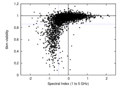
Figure 3: Spectral index distribution plotted against 6km visibility. The dotted lines mark the limits of flat v steep-spectrum on the x-axis and compact v extended sources on the y-axis. Solid line at y = 1 represents the expected values of visibility for unresolved sources. The flux density for 1 GHz is obtained either from SUMSS or NVSS catalogue while 5 GHz is obtained from AT20G follow-up at 4.8 GHz.

Fig. 4 shows the distribution of spectral index ($\alpha_{1}^{4.8}$) for both compact and extended source populations. The mean and standard deviation for Gaussian fits for the compact and extended source populations are given in Table 2.

We can use the spectral index distributions for compact and extended sources plotted in Fig. 4 to find the optimum value of the spectral cut-off to classify the flat and steep-spectrum AGN populations. We get slightly different answers depending on what we want to optimise. The maximum value of the joint probability that both flat and steep-spectrum sources are correctly classified is at $\alpha$ = -0.46 and 80$\%$ of the sources are correctly classified (see Fig. 4). This is independent of the relative number of flat and steep-spectrum sources in the survey, and consequently is only weakly dependent on the survey frequency. This estimate is right between the two values (-0.4 and -0.5) mostly used historically, for consistency we recommend the use of a -0.5 cut-off in future studies. However, if we want to maximise the total number of correctly classified compact sources this does depend on the relative amplitude of the two populations and is dependent on survey frequency varying between $\alpha$ = -0.4 for a survey frequency of 5 GHz to $\alpha$ = -0.6 for a survey frequency of 20 GHz.

Table 2: Gaussian fits to the spectral index distribution of compact and extended sources in Fig. 4.

Survey Frequency	178 MHz	20 GHz
Data	3C∗	AT20G Extended	AT20G Compact
Mean	-0.85	-0.75	0.00
Sigma	0.20	0.23	0.42

*3C values for galaxies for spectral index between 0.75 and 5 GHz from Kellermann et al. (1969).

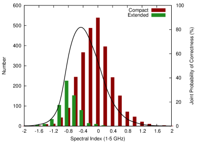
Figure 4: Distribution of Compact and Extended sources over spectral index. The spectral indices are calculated between SUMSS/NVSS 1 GHz and AT20G 4.8 GHz flux densities. Mean spectral indices and dispersions from Gaussian fits to extended and compact source population distributions are given in Table 2. The solid curve is the joint probability of correctness (see text). The histogram for extended sources are shifted by -0.05 to show both populations at the steep-spectrum end.

5 The spectra of sources with 6km visibility

The overall spectral properties of AT20G sources show complex spectral changes and flux density dependence (Massardi et al., 2011). In Fig. 5 we compare the spectra for compact and extended sources for three different frequency ranges. We note the different characteristics between the three frequencies. Spectral index between two frequencies with larger separation is less susceptible to errors due to flux measurement errors than spectral index between two frequencies close to each other. For a 10% error in flux density in Fig. 5, the $\alpha_{5}^{8.6}$ has an error of 0.16, the $\alpha_{8.6}^{20}$ has an error of 0.11 and $\alpha_{1}^{5}$ has an error of 0.06. The 5 and 8 GHz flux density measurements were done within a month of the 20 GHz measurements. Hence, they do not suffer much from variability of compact sources (Massardi et al., 2011) . Although the 1 GHz flux densities were measured at different epochs (between minimum of one to maximum of 15 years), variability is much less at lower frequencies. Hence, errors in flux densities or due to variability do not explain most of the differences seen in the three plots.

In Fig. 5, we note the appearance of a steep-spectrum ‘tail’ for compact sources in the top $\alpha_{8.6}^{20}$ plot. This indicates that while compact sources are mostly flat spectrum at lower frequencies, a fraction of compact sources have steeper spectra between 8 and 20 GHz. It is also evident that the population of compact inverted spectrum sources, sources with spectral index $>$ 1, at lower frequencies shifts to lower spectral index and combines with the main population of the compact sources at higher frequencies. These are compact core sources that are rising at lower frequencies and have either become flat or steep at higher frequencies (e.g. GPS sources) (Sadler et al., 2008).

On the other hand the spectra of extended sources which are well separated by spectral index at low frequencies, have a larger scatter at higher frequencies. A significant fraction of the extended sources move towards the flatter part of the plot at higher frequency. These extended sources are mostly composed of a flat-spectrum core with a steep-spectrum jet, lobe or a hotspot. With increasing frequency, the steep-spectrum part of the sources gets weaker while the compact flat-spectrum cores start to dominate the spectrum. These composite sources show an overall combined flat spectrum but are still extended. This domination of flat-spectrum core should be easily observable by imaging these composite sources at higher frequencies, when only the compact cores should be visible. With increasing frequency, there is a further steepening in the spectra of the extended structures due to energy loss. This is evident in the left part of Fig. 5 with the appearance of a population of very steep extended sources in the $\alpha_{5}^{8.6}$ and $\alpha_{8.6}^{20}$ plots. These two effects combined produce the larger scatter seen in the $\alpha_{8.6}^{20}$ plot of Fig. 5 for extended sources.

It should also be noted that at higher frequencies the spectra of compact sources starts to become indistinguishable from steep-spectrum sources (Fig. 5, $\alpha_{8.6}^{20}$ plot). It is then clear that while the use of spectral index to separate compact and extended sources is valid using lower frequency spectra, it is unable to provide a clean separation of compact and extended sources at higher frequencies.

Figure 5: 6km visibility is plotted against three spectral indices increasing in frequencies with $\alpha_{1}^{4.8}$ at the bottom panel, $\alpha_{4.8}^{8.6}$ at the mid panel and $\alpha_{8.6}^{20}$ at the top panel. The solid vertical line corresponds to spectral index = -0.5 and the solid horizontal lines correspond to 6km visibility = 1.

6 The redshift cut-off and the effect of spectral curvature

Wall et al. (2005) used 379 radio selected QSOs from the Parkes quarter-Jansky flat-spectrum sample selected at 2.7 GHz to study the evolution of flat-spectrum quasars at high redshift. They found that the redshift cut-off is real and is similar to the cut-off observed in optically selected QSOs. Similar results have been reported for cosmic star formation rates. However, Jarvis & Rawlings (2000), using the Parkes half-Jansky flat-spectrum sample selected at 2.7 GHz, argue that because of spectral curvature and the resulting K-correction there is not enough observable volume at high redshift to find the brightest flat-spectrum radio sources, which gives the impression of redshift cut-off. We can use the sub population of compact sources from the AT20G survey, with redshifts, to study the effect of spectral curvature and the K-correction on the redshift cut-off.

A survey at any frequency is biased to the sources that are stronger at the survey frequency. Since this is very obvious, it is not usually considered a bias. At lower frequencies the steep-spectrum sources dominate the population at all luminosities and only contain the rare extremely luminous flat-spectrum sources. Since it is the flat spectrum population that has a high quasar identification rate, this is the sample used to investigate evolution of flat-spectrum quasars (Dunlop & Peacock 1990; Shaver et al. 1996; Jarvis & Rawlings 2000; Vigotti et al. 2003; Wall et al. 2005). Our frequency selection provides a much larger fraction of these sources without introducing a different class of sources, thus, we reduce the bias by having a high frequency selected sample (e.g. Condon 2009).

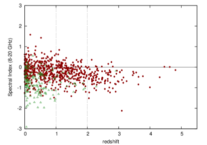
Figure 6: Spectra of compact and extended sources with redshift calculated between 8.6 and 20 GHz. Filled circles represent compact sources and open triangles represent extended sources. The median and standard error for redshift bins, marked by dashed vertical lines, are shown in Table 3.

As noted in Section 2, 838 out of 1460 of AT20G sources with redshift have 4.8 and 8.6 GHz flux densities, 1 GHz NVSS/SUMSS counterparts and 20 GHz flux densities as well as 6km visibility. We use this subsample of sources for the following analysis. Of these, 683 sources are compact by our definition while the remaining 155 sources are extended. The distribution of the redshifts for this AT20G subpopulation is listed in Table 3.

Fig. 6 plots the spectral indices for compact and extended sources between 8.6 and 20 GHz against redshift. It is evident from the plot that extended sources do not show apparent changes in the spectral index over the redshift range. Compact sources, however, show a distinct steepening of their spectra with redshift. It is apparent that a spectral classification is no longer separating the compact and extended sources above redshifts $\sim$ 1.

Since most extended radio sources have close to power-law spectra over a large range of radio frequencies, we do not expect a significant change in spectrum with redshift due to the change in restframe frequency. But as discussed in section 5, compact sources have flat spectra at lower frequencies that gets steeper at higher frequencies. Hence, the spectral indices of compact sources are affected by the redshift effect causing the redshift cut-off as discussed by Jarvis & Rawlings (2000). To test this idea further we use the spectra at different observed frequencies for different redshift ranges.

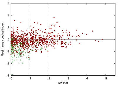
Figure 7: Rest frame spectral index of compact and extended sources. Filled circles represent compact sources and open triangles represent extended sources. All points have been brought close to the rest frame spectral index between 8.6 and 20 GHz by using the spectral index between 8.6 and 20 GHz for all sources below z = 1, using spectral indices between 4.8 and 8.6 GHz for all sources between redshifts 1 and 2 and using spectral index between 1 and 4.8 GHz for all sources with z $\geq$ 2.

The median spectral indices and errors for these redshift ranges are listed in Table 3. Our sources have flux densities measured between four to five frequencies which allows us to calculate, at least, three contiguous spectral indices ($\alpha_{1}^{4.8}$, $\alpha_{4.8}^{8.6}$, $\alpha_{8.6}^{20}$). We take advantage of these spectral points by using the best representative spectra for different redshift bins to remove the effect of redshift and, thus, compare their spectral indices between corresponding rest frequencies. For this, we approximate that the spectral index of $\alpha_{1}^{4.8}$ best represents the redshift bin between 2 and 5 (rest frequencies $\sim$8 and $\sim$14 GHz), $\alpha_{4.8}^{8.6}$ best represents the redshift bin between 1 and 2 (rest frequencies $\sim$10 and $\sim$26 GHz) and $\alpha_{8.6}^{20}$ represents the redshift bin for redshifts up to 1. Plotted in Fig. 7, this essentially brings all spectral indices to $\alpha_{8.6}^{20}$ for comparison in their restframes. We use this simple procedure to preserve the measured values rather than fitting complex spectral shapes to a small number of frequencies.

Table 3: Median spectral indices and standard error for compact and extended sources before (Fig. 6) and after (Fig. 7) redshift corrections. There are only two extended sources in the z $\geq$ 2 bin. The median and standard error are kept inside parentheses to note their limited significance.

Redshift	Compact						Extended
Bins	Number	Uncorrected	Error	Corrected	Error		Number	Uncorrected	Error	Corrected	Error	Total
z $<$ 1	363	-0.17	0.02	-0.17	0.02		138	-0.79	0.05	-0.79	0.05	501
1 $\leq$ z $<$2	211	-0.28	0.03	-0.07	0.03		15	-0.80	0.08	-0.73	0.07	226
z $\geq$ 2	109	-0.49	0.04	0.10	0.05		2	(-0.57)	(0.38)	(-0.24)	(0.02)	111
Total	683						155					838

As is evident in Fig. 7, the redshift correction completely removes the steepening of the spectral indices at higher redshift seen in Fig. 6. Table 3 even indicates that there is now an overall flattening of spectra at higher redshift to 9 sigma confidence. These results show that the spectral curvature plays a dominant role at higher frequencies. To illustrate this further, we have constructed the K-corrected spectra for the entire sample of sources in Fig. 8. Of the sub population of 1377 sources (see Table 1), 1092 sources are compact by our definition and only 671 sources have spectra at four to five frequencies. We calculated the rest frequencies for these sources and normalized them with their average flux density, and plotted them against the rest frequency in Fig. 8. The mean redshift for these 671 compact sources is $\sim$1. The figure confirms the results seen in fig. 6 of Wall et al. (2005) which shows that the spectra of flat-spectrum sources at their rest frames at lower frequencies is predominantly flat suggesting that spectral curvature does not play a significant role at lower frequencies. At lower frequencies up to $\sim$ 5 GHz, we observe that there is a mixture of steep, flat and inverted spectrum sources. It is also clear from the figure that the majority of compact sources remain flat-spectrum up to $\sim$30 GHz in their rest frame frequencies at all redshifts but the trend is then for almost all sources to get steeper. The median normalized flux density for the rest frequency bin between 35 - 45 GHz drops by $\sim$15$\%$ compared to that for the rest frequency bin between 15 - 25 GHz. This explains the effect of spectral steepening at high frequency of compact, and hence, flat-spectrum sources at higher redshifts seen in Fig. 6 and Table 3, as well as the removal of the effect after redshift correction in Fig. 7. The plot also indicates that at lower frequencies, the spectral curvature does not play a significant role. In fact, there is a population of steep-spectrum core-jet sources at the lower frequency end of Fig. 8 which produces the opposite effect. As discussed in Section 5, these compact sources that have steep-spectrum jets at low frequencies are increasingly dominated by their flat-spectrum cores at higher frequencies. The redshift effect of these sources, then, makes them appear flat spectrum at observed lower frequencies at higher redshifts. For sources at high redshifts, this effect negates the effect of spectral steepening of the overall spectra, at lower frequencies.

Thus, the redshift cut-off is affected by the spectral curvature of compact sources as suggested by Jarvis et al. (2001), but this effect only becomes important at higher frequencies ($\nu>$5 GHz) and can be avoided by measuring the spectra at lower frequencies. Fortunately, this is where majority of evolution studies have been done (e.g. Peacock (1985); Dunlop & Peacock (1990); Shaver et al. (1999); Jarvis & Rawlings (2000); Wall et al. (2005)).

So far, we have only discussed the effect of the spectral curvature on the redshift cut-off caused by the use of the spectral index to filter out the compact flat-spectrum sources. However, it is also necessary to see how this effects the number of sources above the flux limit of the survey, referred to by Jarvis & Rawlings (2000) as the observable volume. This cut-off is determined by the survey frequency regardless of the frequency used to measure the spectrum. Low frequency surveys will select against the compact flat-spectrum sources at all redshifts. Higher frequency surveys will have much larger populations of compact sources but they will also have a much stronger redshift cut-off due to spectral curvature.

To evaluate this survey sensitivity effect, we plot the average parameters used in the Jarvis & Rawlings (2000) models, normalized at 2.7 GHz, with our rest frame spectra in Fig. 8. The model is given by a polynomial of the form $y=$ $\rm{log_{10}S_{\nu}}$ = $\Sigma_{i=0}^{2}a_{i}x^{i}$, where $x$ = $\rm{log_{10}}$($\nu$/GHz) with  $a_{1}$ = 0.07 $\pm$ 0.08 and $a_{2}$ = -0.29 $\pm$ 0.06.

It is apparent that the model predicts a much stronger spectral curvature than that obtained for the AT20G compact sources. Even the closest fit, at the extreme of the parameters range, is steeper than that obtained for the AT20G compact sources. We note that the data available to Jarvis & Rawlings (2000) was strongly biased to unusual spectra and GPS sources by the spectral data available and is not representative of the true compact source population. On the basis of their model spectrum Jarvis & Rawlings (2000) predicted a sharp cut-off in the number of observable sources at high redshift and consequently argued that the cut-off seen by Shaver et al. (1996) was not evidence for cosmological evolution. On average, our spectra are at least five times brighter than Jarvis & Rawlings (2000) model, at our higher frequencies which are relevant for the high redshift sources found in lower frequency samples such as those of Jarvis & Rawlings (2000) or Wall et al. (2005). So, even at high redshift the expected number of sources will be larger by a similar fraction at this flux density level. The bias introduced by preferential selection of flat-spectrum sources due to high AT20G survey frequency is appropriate for the high redshift sources where cut-off is seen. Hence, the cut-off reported by Shaver et al. (1996) must be mainly due to cosmological evolution and is not the effect of K-correction on either the number of sources or the ability to make spectral classification. The more detailed analysis of Wall et al. (2005), which incorporated the various selection effects and biases explicitly, also demonstrated the reality of the cosmological evolution component.

We compared the Parkes quarter-Janksy flat-spectrum sample (Jackson et al., 2002) with the AT20G data in the overlapping area of the sky. The PQJFS sample has 804 southern hemisphere sources and actually includes sources with flux densities less than 250 mJy. We have included all sources down to 220 mJy since that corresponds to 100 mJy at 20 GHz for the spectral index cut-off of -0.4. There are 716 PQJFSS sources over the limit of 220 mJy at 2.7 GHz. The cross match of these sources’ positions against the AT20G catalogue (Murphy et al., 2010) finds 640 of these sources and further 31 are found in the AT20G scanning survey catalogue (Hancock et al., 2011) which avoids the incompleteness introduced by the AT20G follow-up observations. We used the updated positions of the sources provided in Jackson et al. (2002), where available, since the original PQJFSS positions are not fully reliable. Thus, our cross-match found a total of 671 (94 $\%$) PQJFSS sources in the AT20G survey. Of the remaining 45 sources, 14 were later found to be extended sources by Jackson et al. (2002) and are not included in their analysis. For the remainder, our literature search finds that 7 are detected at lower frequencies and have steep-spectrum, 9 are known variable sources based on multiple epoch observations and 1 source that has not been detected in any other surveys. The remaining 14 sources (2$\%$) are well within the completeness expected from long term variability noting that the AT20G survey was done $>$ 20 years after the PQJFS survey. Only 3 (0.4$\%$) of these sources have evidence for extreme spectral steepening at high frequency. Hence, we can conclude that we have not lost a significant fraction of sources as a result of spectral steepening which has put them below our survey limit.

603 of the detected sources have 6km visibilities and 548 of them are compact while 55 (9$\%$) are extended, consistent with the overlap in the spectral index distribution shown in Fig. 4. Out of the detected sources, 461 sources have redshift information. The published PQJFS sample has 459 sources in the southern hemisphere with redshifts.

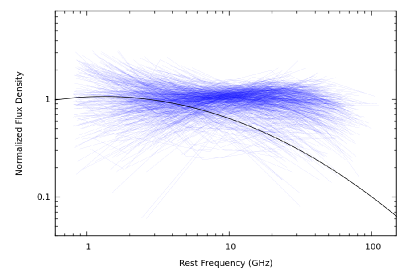
Figure 8: Rest frame radio spectra of 671 compact AT20G sources. Sources have flux density observations at a subset of 0.8, 1.4 and 4.8, 8.6 and 20 GHz. All observed frequencies are converted to the rest frame and the flux densities are normalized by their average flux density over all frequencies present. The solid black line is the fit to the spectra of the most luminous Parkes Half-Jansky Flat-Spectrum sample done by Jarvis & Rawlings (2000) normalized at 2.7 GHz survey frequency.

7 Summary

We summarise the results of this work.

1. 6km visibility, calculated as the ratio of five long baselines to the 10 short baselines of the ATCA in hybrid configurations, provides information on the angular sizes of the extragalactic source population at 20 GHz. It is used to separate the source population into compact and extended sources at subarcsec (0.15 arcsecond) level.

2. 6km visibility provides a firm physical basis for spectral classification into flat and steep-spectrum sources to select compact and extended sources. For spectral indices measured between 1 and 5 GHz, the spectral index of -0.46 is the optimum cut-off between the two populations. However, the traditional cut-off of either -0.4 or -0.5 are almost as good and for consistency, we recommend that -0.5 be used in future studies.

3. 79% of the sources in our survey are compact AGNs which is a result of the high survey frequency. This is very different from low frequency surveys such as NVSS which has only 25% of the flat-spectrum AGN source population.

4. A larger scatter in the spectral index of extended sources is observed at higher frequencies due to the domination of compact cores in core-jet sources as well as the steepening of extended jets due to energy loss. Hence, the use of spectral index at high frequencies is not as effective to select compact and extended sources. Using the radio spectrum below a few gigahertz avoids this problem.

5. The spectral curvature is significant for compact sources, but it only becomes significant at higher frequencies. Below a few gigahertz frequencies, the redshift effect on compact sources is not significant. We note that the general spectral steepening seen above 20 GHz will occur at observed frequencies around 5 GHz, for sources with redshift $>$ 3. Hence, surveys at frequencies $>$ 5 GHz will have a redshift cut-off due to spectral curvature.

6. At high frequencies, the spectra of both compact and extended sources are steep and the two populations become indistinguishable from each other due to the spectral steepening of compact sources by $\sim$ 15% between 20 and 40 GHz.

7. The effect of K-correction shown by Jarvis & Rawlings (2000) is important at high frequencies as discussed by Shaver et al. (1996) and Wall et al. (2005) for flat-spectrum sources and also for steep-spectrum sources (Rigby et al., 2011). However, this should not affect the results of Shaver et al. (1996) and Wall et al. (2005) as they used low frequency spectral index to select compact sources. Hence, the conclusion that the compact sources show a strong redshift cut-off is supported by our data.

   In future, with the information on the completeness of the optical identification and redshifts, it will be possible to explore the density evolution and redshift cut-off of compact AGN without using the spectral index to select compact sources.

This document has been typeset from a TeX/LaTeXfile prepared by the author.

References

- Boyle et al. (1988) Boyle, B. J., Shanks, T., Peterson, B. A. 1988, MNRAS, 235, 935
- Browne et al. (2003) Browne, I. W. A., et al. 2003, MNRAS, 341, 13
- Condon (2009) Condon, J. J. 2009, A&A, 500, 219
- Condon et al. (1998) Condon, J. J., Cotton, W. D., Greisen, E. W., Yin, Q. F., Perley, R. A., Taylor, G. B., Broderick, J. J. 1998, AJ, 115, 1693
- De Breuck et al. (2000) De Breuck, C., van Breugel, W., Röttgering, H. J. A., Miley, G. 2000, A&AS, 143, 303
- de Zotti et al. (2010) de Zotti, G., Massardi, M., Negrello, M., Wall, J. 2010, A&A Rev., 18, 1
- de Zotti et al. (2005) de Zotti, G., Ricci, R., Mesa, D., Silva, L., Mazzotta, P., Toffolatti, L., González-Nuevo, J. 2005, A&A, 431, 893
- Dunlop & Peacock (1990) Dunlop, J. S. Peacock, J. A. 1990, MNRAS, 247, 19
- Hancock et al. (2011) Hancock, P. J., et al. 2011, ArXiv e-prints:1109.1886
- Hasinger et al. (2005) Hasinger, G., Miyaji, T., Schmidt, M. 2005, A&A, 441, 417
- Jackson & Wall (1999) Jackson, C. A. Wall, J. V. 1999, MNRAS, 304, 160
- Jackson et al. (2002) Jackson, C. A., Wall, J. V., Shaver, P. A., Kellermann, K. I., Hook, I. M., Hawkins, M. R. S. 2002, A&A, 386, 97
- Jarvis & Rawlings (2000) Jarvis, M. J. Rawlings, S. 2000, MNRAS, 319, 121
- Jarvis et al. (2001) Jarvis, M. J., Rawlings, S., Willott, C. J., Blundell, K. M., Eales, S., Lacy, M. 2001, MNRAS, 327, 907
- Kellermann et al. (1969) Kellermann, K. I., Pauliny-Toth, I. I. K., Williams, P. J. S. 1969, ApJ, 157, 1
- Larson et al. (2011) Larson, D., et al. 2011, ApJS, 192, 16
- Mahony et al. (2011) Mahony, E. K., et al. 2011, MNRAS, 417, 2651
- Massardi et al. (2010) Massardi, M., Bonaldi, A., Negrello, M., Ricciardi, S., Raccanelli, A., de Zotti, G. 2010, MNRAS, 404, 532
- Massardi et al. (2011) Massardi, M., et al. 2011, MNRAS, 412, 318
- Mauch et al. (2003) Mauch, T., Murphy, T., Buttery, H. J., Curran, J., Hunstead, R. W., Piestrzynski, B., Robertson, J. G., Sadler, E. M. 2003, MNRAS, 342, 1117
- Murphy et al. (2010) Murphy, T., et al. 2010, MNRAS, 402, 2403
- Myers et al. (1995) Myers, S. T., et al. 1995, ApJ, 447, L5+
- O’Dea (1998) O’Dea, C. P. 1998, PASP, 110, 493
- Peacock (1985) Peacock, J. A. 1985, MNRAS, 217, 601
- Rigby et al. (2011) Rigby, E. E., Best, P. N., Brookes, M. H., Peacock, J. A., Dunlop, J. S., Röttgering, H. J. A., Wall, J. V., Ker, L. 2011, MNRAS, 1122
- Sadler et al. (2008) Sadler, E. M., Ricci, R., Ekers, R. D., Sault, R. J., Jackson, C. A., de Zotti, G. 2008, MNRAS, 385, 1656
- Sadler et al. (2006) Sadler, E. M., et al. 2006, MNRAS, 371, 898
- Saikia et al. (2001) Saikia, D. J., Jeyakumar, S., Salter, C. J., Thomasson, P., Spencer, R. E., Mantovani, F. 2001, MNRAS, 321, 37
- Schmidt et al. (1991) Schmidt, M., Schneider, D. P., Gunn, J. E. 1991, in Astronomical Society of the Pacific Conference Series, Vol. 21, The Space Distribution of Quasars, ed. D. Crampton, 109–114, as referenced in Wall et al. 2005
- Shaver (1995) Shaver, P. A. 1995, in Annals of the New York Academy of Sciences, Vol. 759, Seventeeth Texas Symposium on Relativistic Astrophysics and Cosmology, ed. H. Böhringer, G. E. Morfill, & J. E. Trümper, 87–+
- Shaver et al. (1999) Shaver, P. A., Hook, I. M., Jackson, C. A., Wall, J. V., Kellermann, K. I. 1999, in Astronomical Society of the Pacific Conference Series, Vol. 156, Highly Redshifted Radio Lines, ed. C. L. Carilli, S. J. E. Radford, K. M. Menten, & G. I. Langston , 163–+
- Shaver et al. (1996) Shaver, P. A., Wall, J. V., Kellermann, K. I., Jackson, C. A., Hawkins, M. R. S. 1996, Nature, 384, 439
- Tucci et al. (2011) Tucci, M., Toffolatti, L., De Zotti, G., Martinez-Gonzalez, E. 2011, ArXiv e-prints:1103.5707
- Vigotti et al. (2003) Vigotti, M., Carballo, R., Benn, C. R., De Zotti, G., Fanti, R., Gonzalez Serrano, J. I., Mack, K.-H., Holt, J. 2003, ApJ, 591, 43
- Wall (1977) Wall, J. V. 1977, in IAU Symposium, Vol. 74, Radio Astronomy and Cosmology, ed. D. L. Jauncey, 55–+
- Wall et al. (2005) Wall, J. V., Jackson, C. A., Shaver, P. A., Hook, I. M., Kellermann, K. I. 2005, A&A, 434, 133
- Winn et al. (2000) Winn, J. N., et al. 2000, AJ, 120, 2868