The $K\pi$ form factors from Analyticity and Unitarity

Abstract

Analyticity and unitarity techniques are employed to obtain bounds on the shape parameters of the scalar and vector form factors of semileptonic $K_{l3}$ decays. For this purpose we use vector and scalar correlators evaluated in pQCD, a low energy theorem for scalar form factor, lattice results for the ratio of kaon and pion decay constants, chiral perturbation theory calculations for the scalar form factor at the Callan-Treiman point and experimental information on the phase and modulus of $K\pi$ form factors up to an energy $t_{\rm in}=1{\rm GeV}^{2}$. We further derive regions on the real axis and in the complex-energy plane where the form factors cannot have zeros.

1 Introduction

$K_{l3}$ decays are important for determining the matrix element $V_{us}$, for recent reviews, see [1, 2] of the Cabibbo-Kobayashi-Maskawa (CKM) which in turn is crucial for testing the unitarity of the CKM matrix. Information on the experimental sector is rich, in particular for the $K_{\ell 3}$ decay rates, which were measured by a number of experiments BNL-E865 [3], KLOE [4], ISTRA+ [5], KTEV [6] and more recently a new analysis by NA48 [7]. Recent lattice studies have also been carried out, see refs.[8, 9, 10, 11].

The decay of a kaon to a pion, a charged lepton and a neutrino is described by the matrix element

$$\langle\pi^{0}(p^{\prime})|\overline{s}\gamma_{\mu}u|K^{+}(p)\rangle=\frac{1}{\sqrt{2}}[(p^{\prime}+p)_{\mu}f_{+}(t)+(p-p^{\prime})_{\mu}f_{-}(t)],$$ (1)

where $f_{+}(t)$ is the vector form factor and the combination

$$f_{0}(t)=f_{+}(t)+\frac{t}{M_{K}^{2}-M_{\pi}^{2}}f_{-}(t)$$ (2)

is known as the scalar form factor. The expansion at $t=0$

$$f_{k}(t)=f_{+}(0)\left(1+\lambda_{k}^{\prime}\,\frac{t}{M_{\pi}^{2}}+\frac{1}{2}\lambda_{k}^{\prime\prime}\,\frac{t^{2}}{M_{\pi}^{4}}+\cdots\right),$$ (3)

defines the slope $\lambda_{k}^{\prime}$ and the curvature $\lambda_{k}^{\prime\prime}$ parameters where $k=0$ denotes the scalar and $k=+$ denotes the vector form factor. The precise determination of the element $|V_{us}|$ depends on how accurate the parametrization of the form factor is. To improve the precision and to provide bounds on the shape parameters of the form factors, we use inputs coming from certain low energy theorems, perturbative QCD, lattice computations and chiral perturbation theory. Our techniques allow us to incorporate the phase and modulus information of the form factors. We also apply the technique to find regions on the real axis and in the complex $t$-plane where zeros are excluded. The knowledge of zeros is of interest, for instance, for the dispersive methods (Omnès-type representations) and for testing specific models of the form factors. For more details, see refs. [12, 13, 14, 15].

2 Formalism

The formalism described in [12, 13, 14] and in the contribution to these Proceedings [16] , exploits an integral of the type

$$\int^{\infty}_{t_{+}}dt\ \rho_{+,0}(t)|f_{+,0}(t)|^{2}\leq I_{+,0},$$ (4)

along the unitarity cut, whose upper bound is known from a dispersion relation, satisfied by a certain QCD correlator. For the scalar form factor this reads

$$\chi_{{}_{0}}(Q^{2})\equiv\frac{\partial}{\partial q^{2}}\left[q^{2}\Pi_{0}\right]=\frac{1}{\pi}\int_{t_{+}}^{\infty}\!dt\,\frac{t{\rm Im}\Pi_{0}(t)}{(t+Q^{2})^{2}}\,,$$ (5)

$${\rm Im}\Pi_{0}(t)\geq\frac{3}{2}\frac{t_{+}t_{-}}{16\pi}\frac{[(t-t_{+})(t-t_{-})]^{1/2}}{t^{3}}|f_{0}(t)|^{2}\,,$$ (6)

with $t_{\pm}=(M_{K}\pm M_{\pi})^{2}$. Analogues expression, involving a suitable correlator denoted by $\chi_{1}(Q^{2})$, can be written down for the vector form factor. We can now use the conformal map $t\to z(t)$

$$z(t)=\frac{\sqrt{t_{+}}-\sqrt{t_{+}-t}}{\sqrt{t_{+}}+\sqrt{t_{+}-t}}\,,$$ (7)

that maps the cut $t$-plane onto the unit disc $|z|<1$ in the $z\equiv z(t)$ plane, with $t_{+}$ mapped onto $z=1$, the point at infinity to $z=-1$ and the origin to $z=0$. Using this map, we cast eqn.(4) into a canonical form, incorporate phase and modulus information as well as the Callan-Treiman relations and finally employ a determinant for obtaining bounds on the shape parameters and for finding regions of excluded zeros in the complex $t$-plane.

3 Inputs

The essential inputs of our formalism, the vector $\chi_{1}(Q^{2})$ and the scalar $\chi_{0}(Q^{2})$ correlators, can be calculated in perturbative QCD up to order $\alpha_{s}^{4}$ for $Q^{2}>>\Lambda^{2}_{QCD}$ [17, 18]. We get $\chi_{1}(2\,\text{GeV})=(343.8\pm 51.6)\times 10^{-5}\,{\rm GeV}^{-2}$ and $\chi_{0}(2\,\text{GeV})=(253\pm 68)\times 10^{-6}$, see also [12]. An improvement can be achieved when we implement theoretical and experimental information into the formalism of unitarity bounds. The first improvement comes when we use the the value of vector form factor at zero momentum transfer. Recent determinations from the lattice give $f_{+}(0)=0.964(5)$ [19]. We can also use two low energy theorems, namely soft pion and soft kaon theorems, for the improvement of the bounds on the slope and curvature parameters in the scalar case. The soft pion theorem relates the value of scalar form factor at first Callan-Treiman piont $\Delta_{K\pi}\equiv M_{K}^{2}-M_{\pi}^{2}$ to the ratio $F_{K}/F_{\pi}$ of the decay constants [20, 21]:

$$f_{0}(\Delta_{K\pi})=F_{K}/F_{\pi}+\Delta_{CT}.$$ (8)

Recent lattice evaluations with $N_{f}$ = 2 + 1 flavors of sea quarks give $F_{K}/F_{\pi}=1.193\pm 0.006$ [8, 9]. In the isospin limit, $\Delta_{CT}=-3.1\times 10^{-3}$ to one loop [22] and $\Delta_{CT}\simeq 0$ to two-loops in chiral perturbation theory [23, 24, 25].

At $\bar{\Delta}_{K\pi}(=-\Delta_{K\pi})$, a soft-kaon result [26] relates the value of the scalar form factor to $F_{\pi}/F_{K}$

$$f_{0}(-\Delta_{K\pi})=F_{\pi}/F_{K}+\bar{\Delta}_{CT}.$$ (9)

A calculation in ChPT to one-loop in the isospin limit [22] gives $\bar{\Delta}_{CT}=0.03$, but the higher order ChPT corrections are expected to be larger in this case. As discussed in [14], due to the poor knowledge of $\bar{\Delta}_{CT}$, the low-energy theorem eqn.(9) is not useful for further constraining the shape of the $K_{\ell 3}$ form factors at low energies. On the other hand, we obtain from the same machinery, the stringent bound on the quantity $\bar{\Delta}_{CT}$ which is $-0.046\leq\bar{\Delta}_{CT}\leq 0.014$.

Further improvement of the bounds can be achieved if the phase of the form factor along the elastic part of the unitarity cut is known from an independent source. In our calculations we use below $t_{\rm in}$ the phases from [27, 28] for the scalar form factor, and from [29, 30] for the vector form factor. Above $t_{\rm in}$ we take $\delta(t)$ Lipschitz continuous, i.e., a smooth function approaching $\pi$ at high energies. The results are independent of the choice of the phase for $t>t_{\rm in}$. We can further improve the bounds if the modulus of the form factor is known along the unitarity cut, $t\leq t_{\rm in}$: we can shift the branch point from $t_{\pm}$ to $t_{in}$ by subtracting the low energy integral from the integral Eq. (4). In order to estimate the low-energy integral, which is the value of the integral contribution from $t_{+}$ to $t_{\rm in}$, see for expressions ref.[13], we use the Breit-Wigner parameterizations of $|f_{+}(t)|$ and $|f_{0}(t)|$ in terms of the resonances given by the Belle Collaboration [31] for fitting the rate of $\tau\to K\pi\nu$ decay. The above leads to the value $31.4\times 10^{-5}\,{\rm GeV}^{-2}$ for the vector form factor and $60.9\times 10^{-6}$ for the scalar form factor. By combining with the values $I_{+,0}$, we obtain the new upper bound on the integral Eq. (4) from $t_{\rm in}$ to $\infty$, $I_{+}^{\prime}=(312\pm 69)\times 10^{-5}{\rm GeV}^{-2}$ and $I_{0}^{\prime}=(192\pm 90)\times 10^{-6}$.

Figure 1: The allowed range for the slope of the scalar form factor, when we include phase, modulus and the CT constraint (yellow band). The grey band shows the range without the CT constraint.

Figure 2: Allowed domain for the slope and curvature of the scalar form factor, using the normalization $f_{+}(0)=0.962$, the value $f_{0}(\Delta_{K\pi})=1.193$, and phase and modulus information up to $t_{\rm in}=(1\,\mbox{GeV})^{2}$.

4 Results

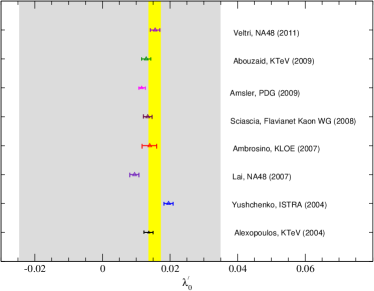
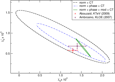
In Figs. 1 and 2, the constraints for the scalar form factor are represented together with experimental information from various experiments. As shown in Fig. 1, the slope $\lambda_{0}^{\prime}$ of the scalar form factor, predicted by NA48 (2007) is not consistent with our predictions (yellow band) which are obtained by taking into account the phase, modulus as well as the CT constraint. Nevertheless our predicted range for the slope is well-respected by the recent 2011 analysis by NA48 [7] .

Figure 3: The best constraints for the slope and curvature of the vector form factor in the slope-curvature plane, where the allowed region is the interior of the ellipse.

The value of $\lambda_{0}^{\prime}$ for this new determination by the NA48 reads $\lambda_{0}^{\prime}=(15.6\pm 1.2\pm 0.9)\times 10^{-3}$. On the theoretical side, the prediction of ChPT to two loops gives $\lambda_{0}^{\prime}=(13.9_{+1.3}^{-0.4}\pm 0.4)\times 10^{-3}$ and $\lambda_{0}^{\prime\prime}=(8.0_{+0.3}^{-1.7})\times 10^{-4}$ which are consistent with our results within errors as shown in Fig. 2. For the central value of the slope $\lambda_{0}^{\prime}$ given above, the range of $\lambda_{0}^{\prime\prime}$ is $(8.24\times 10^{-4},8.42\times 10^{-4})$. The corresponding theoretical predictions are $\lambda_{0}^{\prime}=(16.00\pm 1.00)\times 10^{-3}$, $\lambda_{0}^{\prime\prime}=(6.34\pm 0.38)\times 10^{-4}$ obtained from dispersion relations.

Figure 4: Domain without zeros for the scalar form factor: the small domain is obtained without including phase and modulus in the elastic region, the bigger one using phase, modulus and CT constraint.

Figure 5: Domain without zeros for the vector form factor: the small domain is obtained without including phase and modulus in the elastic region, the bigger one using phase and modulus.

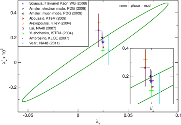
Comparison of the experimental results with our constraints for the vector form factor is shown in Fig. 3. We find that except for the results from NA48 (2007) and KLOE, which have curvatures slightly larger than the allowed values, the experimental data satisfy our constraints. The new results from NA48 [7] provide a curvature which overlaps with our constraints while the slope lies completely within our domain as seen in the figure. We also note that the theoretical predictions $\lambda_{+}^{\prime}=(24.9\pm 1.3)\times 10^{-3}$, $\lambda_{+}^{\prime\prime}=(1.6\pm 0.5)\times 10^{-3}$ obtained from ChPT to two loops, and $\lambda_{+}^{\prime}=(26.05_{-0.51}^{+0.21})\times 10^{-3}$, $\lambda_{+}^{\prime\prime}=(1.29_{-0.04}^{+0.01})\times 10^{-3}$, and $\lambda_{+}^{\prime}=(25.49\pm 0.31)\times 10^{-3}$, $\lambda_{+}^{\prime\prime}=(1.22\pm 0.14)\times 10^{-3}$ obtained from dispersion relations are consistent with the constraint. For more results, see [12].

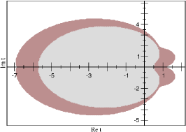
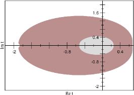
We can also extend our technique to derive regions in the complex plane where the form factors can not have zeros. For the $K\pi$ form factors, the influence of possible zeros in the context of Omnès dispersive representations has been analyzed in [30]. The absence of zeros is assumed in the recent analysis of KTeV data reported in [6]. In Fig. 5 we show the region where zeros of the scalar form factors are excluded. The formalism rules out zeros in the physical region of the kaon semileptonic decay. In the case of complex zeros, we have obtained a rather large region where they cannot be present. In the case of the vector form factor, the analysis of [30] using data from $\tau$ decay concludes that complex zeros cannot be excluded, due to the lack of information on the phase of the form factor in the inelastic region. However our formalism is independent of phase information in the inelastic region and leads without any assumptions to a rather large domain where complex zeros are excluded. For the vector form factor, fig. 5 shows the region where complex zeros are excluded. For more results, see [12].

5 Conclusion

We have derived stringent constraints on the shape parameters of the form factors of $K_{l3}$ decay which is the best source for the extraction of CKM matrix element $V_{us}$. The results are promising and stringent especially in the case of the scalar form factor. The most recent results from NA48 [7] is consistent with our prediction for the slope of scalar form factor and restricts the range of the slope to $\sim 0.01-0.02$. We have also excluded zeros in a rather large domain at low energies both for the scalar and vector form factor. The Callan-Treiman input provides an additional constraint in the case of the scalar form factor and as a result excludes a larger domain of the energy plane where zeros can exist. Thus, this work represents a powerful application of the theory of unitarity bounds, which relies not so much on experimental information, but on theoretical inputs from perturbative QCD, low energy theorems and lattice calculations. It provides a powerful consistency check on determinations of shape parameters from phenomenology and experimental analyses.

References

- [1] M. Antonelli, V. Cirigliano, G. Isidori, F. Mescia, M. Moulson, H. Neufeld, E. Passemar and M. Palutan et al., Eur. Phys. J. C 69, 399 (2010). [arXiv:1005.2323 [hep-ph]].
- [2] V. Cirigliano, G. Ecker, H. Neufeld, A. Pich and J. Portoles, arXiv:1107.6001 [hep-ph].
- [3] A. Sher et al., Phys. Rev. Lett. 91, 261802 (2003) [arXiv:hep-ex/0305042].
- [4] F. Ambrosino et al. [KLOE Collaboration], Phys. Lett. B 636, 166 (2006). [arXiv:hep-ex/0601038].
- [5] V. I. Romanovsky et al., arXiv:0704.2052 [hep-ex].
- [6] E. Abouzaid et al. [KTeV collaboration], Phys. Rev. D 81, 052001 (2010). [arXiv:0912.1291 [hep-ex]].
- [7] M. Veltri, arXiv:1101.5031 [hep-ex].
- [8] L. Lellouch, PoS LATTICE 2008, 015 (2009). [arXiv:0902.4545 [hep-lat]].
- [9] S. Durr et al., Phys. Rev. D 81, 054507 (2010). [arXiv:1001.4692 [hep-lat]].
- [10] G. Colangelo et al., Eur. Phys. J. C 71, 1695 (2011). [arXiv:1011.4408 [hep-lat]].
- [11] A. Ramos et al., arXiv:1101.3968 [hep-lat].
- [12] G. Abbas, B. Ananthanarayan, I. Caprini and I. Sentitemsu Imsong, Phys. Rev. D 82, 094018 (2010). [arXiv:1008.0925 [hep-ph]].
- [13] G. Abbas, B. Ananthanarayan, I. Caprini, I. Sentitemsu Imsong and S. Ramanan, Eur. Phys. J. A 45, 389 (2010). [arXiv:1004.4257 [hep-ph]].
- [14] G. Abbas, B. Ananthanarayan, I. Caprini, I. Sentitemsu Imsong and S. Ramanan, Eur. Phys. J. A 44, 175 (2010). [arXiv:0912.2831 [hep-ph]].
- [15] G. Abbas, B. Ananthanarayan, I. Caprini and I. S. Imsong, arXiv:1112.4270 [hep-ph].
- [16] B. Ananthanarayan, I. Caprini, Constraining Form Factors with the Method of Unitarity Bounds, these Proceedings.
- [17] P. A. Baikov, K. G. Chetyrkin and J. H. Kuhn, Phys. Rev. Lett. 96, 012003 (2006). [hep-ph/0511063].
- [18] P. A. Baikov, K. G. Chetyrkin and J. H. Kuhn, Phys. Rev. Lett. 101, 012002 (2008). [arXiv:0801.1821 [hep-ph]].
- [19] P. A. Boyle, A. Juttner, R. D. Kenway, C. T. Sachrajda, S. Sasaki, A. Soni, R. J. Tweedie and J. M. Zanotti, Phys. Rev. Lett. 100, 141601 (2008). [arXiv:0710.5136 [hep-lat]].
- [20] C. G. Callan and S. B. Treiman, Phys. Rev. Lett. 16, 153 (1966).
- [21] R. F. Dashen and M. Weinstein, Phys. Rev. Lett. 22, 1337 (1969).
- [22] J. Gasser and H. Leutwyler, Nucl. Phys. B 250, 517 (1985).
- [23] A. Kastner and H. Neufeld, Eur. Phys. J. C 57, 541 (2008). [arXiv:0805.2222 [hep-ph]].
- [24] J. Bijnens and P. Talavera, Nucl. Phys. B 669, 341 (2003). [hep-ph/0303103].
- [25] J. Bijnens and K. Ghorbani, arXiv:0711.0148 [hep-ph].
- [26] R. Oehme, Phys. Rev. Lett. 16, 215 (1966).
- [27] P. Buettiker, S. Descotes-Genon and B. Moussallam, Eur. Phys. J. C 33, 409 (2004). [hep-ph/0310283].
- [28] B. El-Bennich, A. Furman, R. Kaminski, L. Lesniak, B. Loiseau and B. Moussallam, Phys. Rev. D 79, 094005 (2009). [Erratum-ibid. D 83, 039903 (2011) ] [arXiv:0902.3645 [hep-ph]].
- [29] B. Moussallam, Eur. Phys. J. C 53, 401 (2008). [arXiv:0710.0548 [hep-ph]].
- [30] V. Bernard, M. Oertel, E. Passemar and J. Stern, Phys. Rev. D 80, 034034 (2009). [arXiv:0903.1654 [hep-ph]].
- [31] D. Epifanov et al. [Belle Collaboration], Phys. Lett. B 654, 65 (2007). [arXiv:0706.2231 [hep-ex]].