The improved Gaussian approximation Calculation of Bogoliubov Mode in One Dimensional Bosonic Gas

Abstract

In this paper, we study the homogeneous one-dimensional bosonic gas interacting via a repulsive contact potential by using the improved Gaussian approximation. We obtain the gapless excitation spectrum of Bogoliubov mode. Our result is in good agreement with the exact numerical calculation based on the Bethe ansatz. We speculate that the improved Gaussian approximation could be a quantitatively good approximation for higher dimensional systems.

I Introduction

Since the concept of Bose-Einstein condensation (BEC) was originally put forward by Bose and Einstein, the dilute Bose gas, as a many-body system which displays macroscopic quantum phenomena such as superfluidity, has been extensively studied theoretically. The microscopic description of BEC started with Bogoliubov theorykey-1 ; key-2 ; key-3 ; key-4 , in which the destruction and creation operators for the macroscopically-occupied lowest-energy mode is specially treated as c numbers, known as Bogoliubov replacement. Based on Bogoliubov replacement, the Green’s function methods were applied to a dilute Bose gas at zero temperature key-5 ; key-6 ; key-7 . Hugenholtz and Pines key-7 showed that for a repulsive interaction, the pole of the one-particle Green’s function, approaches zero for zero momentum, which means a gapless excitation spectrum (usually we call it as Goldstone theorem key-41 ). P.C. Hohenberg and P.C. Martin described BEC as spontaneous global $U(1)$ symmetry breaking by introducing external sources, which are set negligibly small in the end key-8 . The interpretation of BEC as symmetry breaking makes the quantum field-theoretic treatment very convenient, in which the expectation value of the field operator describes the density as well as the wavefunction of the condensed bosons and hence is also called ”macroscopic wavefunction”. The effective action approach key-33 ; Baym ; key-34 ; key-35 ; key-36 is usually employed and kinds of approximations can be easily formulated in this framework, such as Bogoliubov approximation, Popov approximation and Hartree-Fock Bogoliubov (HFB) approximation as discussed in detail in the references key-9 ; key-10 ; key-11 ; key-12 ; key-13 ; key-14 .

However for the bosonic model, if we use the simplest non-perturbative calculation, Hartree-Fock Bogoliubov (HFB) approximation, the spectrum obtained is gapped even in the broken phase. Goldstone theorem is violated in such approximation key-8 ; key-9 . Though in the Popov approximation, the spectrum remains gapless, the method is not self-consistent and we will also show that we can not apply this method to one dimensional bosonic model. $\ \Phi$ derivable theory, self-consistent approximation method beyond HFB, including some higher two particle irreducible (2PI) diagrams to the effective action, is often used in studying BEC systems. The spectrum obtained in the $\Phi$ derivable theory is also gapped Hendrik .

In the self-consistent theories such as Hartree-Fock Bogoliubov (HFB) approximation, the Ward identity from $U(1)$ symmetry is not preserved due to partial resummations of some Feymann diagrams. Therefore, the Goldstone theorem is violated and the resulting excitation spectrum is gapped even in the symmetry breaking phase.  In order to preserve the Ward identity, we should incorporate the contributions of some other Feymann diagrams and thereby remove the gap Rosenstein ; Okopinska ; Hendrik . It is called ”covariant Gaussian approximation” in Rosenstein and we will call it ”improved Gaussian approximation” (IGA). In principle we can apply similar method to the $\Phi$ derivable theory beyond HFB (we will call it the improved $\Phi$ derivable theory, or IDT in short), but the theory becomes too complex (involving integral equations which can not be solved analytically) Hendrik .

In recent years, interest in 1D Bose gas has been revived due to its experimental realization with ultracold bosonic atoms key-22 ; key-23 ; key-24 ; key-25 . In one dimension (1D), at finite temperature, the excitation spectra are gapped. However, the 1D Bose gas at zero temperature contains gapless spectra and the system is algebraic long range order. In a trapped 1D gas, the Bose-Einstein condensation (BEC) regimes of a true condensate, quasicondensate regime and the regime of a trapped Tonks gas (gas of impenetrable bosons) at finite temperature have been identified in ShlyapnikovPRL2000 . The stability and phase coherence of trapped 1D Bose gases was studied in ShlyapnikovPRL2003 . Most of the other relevant works are summarized in the review article key-26 . In highly anisotropic traps, where the axial motion of the atoms is weakly confined while the radial motion is frozen by the tight transverse confinement, the shape of the Bose-condensed systems reduces to one dimension. If the characteristic range of the interatomic potential is much smaller than the typical length of the radial extension, the system can be described by the Lieb-Liniger model key-19 ; key-20 , in which the contact potential strength $g_{1D}$ is given by $g_{1D}=-\frac{2\hbar^{2}}{ma_{1D}}$ with $a_{1D}$ being the 1D scattering lengthkey-27 ; key-28 . The Lieb-Liniger model can be exactly solved by the Bethe ansatz and two types of excitations (named Type I and Type II) have been found. Type I excitations are gapless with a linear dispersion in the long wavelength limit and reduce to the Bogoliubov excitations in the weak coupling limit. Type II excitations, the Fermionic excitations which are prominent in the strong coupling regime, have no equivalent in the Bogoliubov theory. J. S. Caux et al.key-29 studied the one-particle dynamical correlation function of the Lieb–Liniger model by using the ABACUS method key-30 , for a wide range of values of the interaction parameter.

In this paper we will apply IGA to the 1D Bose gas at zero temperature. This system can be described by the Lieb-Liniger model (LLM), which has been exactly solved by the Bethe ansatz. We can compare the result of the IGA method with the exact one in order to test the precision and validity of the IGA method. In the future, we shall apply IGA to 2D or 3D Bose gas at finite temperature, as in high dimension we can not apply the Bethe ansatz method to obtain the exact solution, IGA or IDT is the only approach we can rely on. In higher dimension, the quantum and thermal fluctuations are weaker than in 1D, the result obtained by IGA or IDT should be better qualitatively and quantitatively than that in 1D.

In this paper, we shall study LLM by using IGA, and focus our attention on the excitation spectrum. We will follow Rosenstein and present IGA method by solving Dyson-Schwinger equations which are generated by functional differentiation of the effective action.

We will show that only the Bogoliubov excitation spectrum (or Type I excitation) can be obtained by IGA. By comparing with the results of the Bogoliubov approximation and Type I excitation based on the exact solution key-19 ; key-29 , we find that the spectrum obtained in this way is good improvement to the spectrum in the Bogoliubov approximation. In order to obtain Type II excitation, we speculate that we shall use more general $\Phi$ derivable theory beyond IGA (we will leave it as our future work). If we study high dimension Bosonic system, there will be no Type II excitation, IGA will give more accurate results quantitatively.

The rest of the paper is organized as follows. In section II we review the basic formulation of one particle irreducible (1PI) effective action theory and the Dyson-Schwinger equations. We also present the 1D bosonic model and the Dyson-Schwinger equations for 1D bosonic model in this section. In section III we review the traditional approximations, such as Bogoliubov approximation, HFB approximation and Popov approximation. In section IV, we present improved Gaussian approximation and obtain an improved gapless excitation spectrum. In section V we make a comparison with the exact solution of the 1D bosonic model key-19 ; key-29 . Finally, we give a summary and the conclusions. We put $\hbar=k_{B}=1$ throughout the paper with $k_{B}$ the Boltzmann constant.

II The Dyson-Schwinger equations for 1D bosonic model

In this section we shall present the general formulations and the model, and set up all the notations and definitions. We shall start with the thermodynamic partition function and set the temperature to zero in the end. For a bosonic system, the grand canonical partition function takes the form key-38

$$\mathcal{Z}=\int\mathcal{D}[\psi^{\ast}\psi]e^{-S[\psi^{\ast},\psi]}$$ (1)

with the classical action $S[\psi^{\ast},\psi]$ given by

$$\int_{0}^{\beta}d\tau\int d^{D}\mathbf{x}\left(\psi^{\ast}\partial_{\tau}\psi-\mu\psi^{\ast}\psi+\mathcal{H}\left[\psi^{\ast},\psi\right]\right)$$ (2)

where $\beta=\frac{1}{k_{B}T}$ , $\mu$ is the chemical potential and $\mathcal{H}\left[\psi^{\ast},\psi\right]$ is the Hamiltonian density, $D$ is the dimension of position space (the formulation is valid for arbitary $D$, however in this paper, we will only carry out calculations for 1D). In order to obtain the correlation functions of field operators, a generating functional is defined by coupling fields to an external source,

$$\mathcal{Z}[J^{\ast},J]=\int\mathcal{D}[\psi^{\ast},\psi]e^{-\left(S[\psi^{\ast},\psi]+J^{\ast}\psi+J\psi^{\ast}\right)},$$ (3)

where $J^{\ast}\psi$ is a shorthand for $\int_{0}^{\beta}d\tau\int d^{D}\mathbf{x}J^{\ast}(\mathbf{x},\tau)\psi(\mathbf{x},\tau)$ and similarly for $J\psi^{\ast}$. The connected generating functional is defined as

$$W[J^{\ast},J]=-\ln\mathcal{Z}[J^{\ast},J].$$ (4)

The one-point expectation value of the field operators can be obtained by the derivatives of the generating functional with respect to the external source,

$$\varphi(\mathbf{x},\tau) = \frac{\delta W[J^{\ast},J]}{\delta J^{\ast}(\mathbf{x},\tau)}$$

$$\varphi^{\ast}(\mathbf{x},\tau) = \frac{\delta W[J^{\ast},J]}{\delta J(\mathbf{x},\tau)}$$ (5)

where $\varphi(\mathbf{x},\tau)=\left\langle\psi(\mathbf{x},\tau)\right\rangle$, $\varphi^{\ast}(\mathbf{x},\tau)=\left\langle\psi^{\ast}(\mathbf{x},\tau)\right\rangle$ with

$$\left\langle\cdots\right\rangle\equiv\frac{1}{\mathcal{Z}[J^{\ast},J]}\int\mathcal{D}[\psi^{\ast},\psi]\cdots e^{-\left(S[\psi^{\ast},\psi]+J^{\ast}\psi+J\psi^{\ast}\right)}.$$ (6)

Successive derivatives generate multi-point correlation functions, for instance,

$$\frac{\delta^{2}W}{\delta J(x)\delta J^{\ast}(y)}=-\left\langle\psi^{\ast}(x)\psi(y)\right\rangle_{c}$$ (7)

where $x\equiv(\mathbf{x},\tau)$, $y\equiv(\mathbf{y},\tau^{\prime})$ and the connected Green’s function $\left\langle\psi^{\ast}(x)\psi(y)\right\rangle_{c}=$ $\left\langle\psi^{\ast}(x)\psi(y)\right\rangle-\left\langle\psi^{\ast}(x)\right\rangle\left\langle\psi(y)\right\rangle$. For notation compactness, we define

$$(J,\,J^{\ast}) \equiv (J_{1},\,J_{2}),(\psi^{\ast},\psi)\equiv(\psi_{1},\psi_{2}),(\varphi^{\ast},\varphi)\equiv(\varphi_{1},\varphi_{2}),$$

$$G_{mn}(x,y) \equiv \left\langle\psi_{m}(x)\psi_{n}(y)\right\rangle_{c},$$ (8)

where $m=1,2$, $n=1,2$. $G_{mn}(x,y)$ is related to $W[J^{\ast},J]$ by the following equation,

$$G_{mn}(x,y)=-\frac{\delta^{2}W}{\delta J_{m}(x)\delta J_{n}(y)}.$$ (9)

The 1PI effective action is defined by the Legendre transformation,

$$\Gamma[\varphi^{\ast},\varphi]=W[J^{\ast},J]-J^{\ast}\varphi-J\varphi^{\ast},$$ (10)

which is a functional of the field expectation $\varphi^{\ast}$and $\varphi$. In analogy with Eq.(5) the external source can be obtained by the derivatives of the effective action with respect to the one-point expectation of the field operators,

$$\frac{\delta\Gamma[\varphi^{\ast},\varphi]}{\delta\varphi(\mathbf{x},\tau)} = -J^{\ast}(\mathbf{x},\tau),$$

$$\frac{\delta\Gamma[\varphi^{\ast},\varphi]}{\delta\varphi^{\ast}(\mathbf{x},\tau)} = -J(\mathbf{x},\tau).$$ (11)

The effective action is the generating functional for vertex functions. Using the chain rule to calculate $\frac{\delta\varphi_{m}(x)}{\delta\varphi_{n}(y)}$, we have

$$\frac{\delta\varphi_{m}(x)}{\delta\varphi_{n}(y)} = \sum_{i}\int dz\frac{\delta\varphi_{m}(x)}{\delta J_{i}(z)}\frac{\delta J_{i}(z)}{\delta\varphi_{n}(y)}$$ (12)

$$= -\sum_{i}\int dz\frac{\delta^{2}W}{\delta J_{m}(x)\delta J_{i}(z)}\frac{\delta^{2}\Gamma}{\delta\varphi_{i}(z)\delta\varphi_{n}(y)}.$$

On the other hand,

$$\frac{\delta\varphi_{m}(x)}{\delta\varphi_{n}(y)}=\delta_{mn}\delta(x-y).$$ (13)

Thus by combining Eqs.(12)(13) one obtains

$$\sum_{i}\int dzG_{mi}(x,z)\Gamma_{in}(z,y)=\delta_{mn}\delta(x-y)$$ (14)

where $\Gamma_{mn}(x,y)\equiv\frac{\delta^{2}\Gamma[\varphi_{1},\varphi_{2}]}{\delta\varphi_{m}(x)\delta\varphi_{n}(y)}$ and $G_{mn}(x,y)$ is defined in Eq.(8). The 1PI effective action $\Gamma[\varphi^{\ast},\varphi]$ can be approximately obtained by loop expansion key-39 .

Dyson-Schwinger equations can be obtained by using the following identity,

$$\int\mathcal{D}[\psi^{\ast},\psi]\frac{\delta}{\delta\psi^{\ast}(x)}e^{-\left(S[\psi^{\ast},\psi]+J^{\ast}\psi+J\psi^{\ast}\right)}=0,$$ (15)

which leads to

$$\left\langle\frac{\delta S[\psi^{\ast},\psi]}{\delta\psi^{\ast}(x)}\right\rangle+J(x)=0.$$ (16)

Derivatives of Eq.(16) with respect to the average field $\varphi_{m}(x)$ shall produce a series of Dyson-Schwinger equations, such as

$$\frac{\delta}{\delta\varphi(y)}\left\langle\frac{\delta S[\psi^{\ast},\psi]}{\delta\psi^{\ast}(x)}\right\rangle+\frac{\delta}{\delta\varphi(y)}J(x)=0.$$ (17)

Successive functional derivatives with respect to $\varphi\left(z\right)$ yield higher order Dyson-Schwinger equations, which involve the correlation functions of more field operators. Therefore, the infinite Dyson-Schwinger equations must be truncated to form a set of closed equations in order to carry out any calculations. Let us term Eq.(16) as the first Dyson-Schwinger equation and Eq.(17) as the second Dyson-Schwinger equation.

We apply the Dyson-Schwinger formalism to a system of one-dimensional bosonic gas interacting via a repulsive contact potential, described by the Lieb-Liniger Hamiltonian

$$H=-\sum_{i=1}^{N}\left(\partial^{2}/\partial x_{i}^{2}\right)+g\sum_{i<j}^{N}\delta(x_{i}-x_{j}),$$ (18)

where the mass of the particle has been set to $2m=1$ and $g$ is the contact interaction strength, which is related to the 1D scattering length experimentally. The second quantization form reads

$$\hat{H}=\int d^{D}\mathbf{x}\left(\psi^{\dagger}(\mathbf{x})(-\nabla^{2})\psi(\mathbf{x})+\frac{1}{2}g\psi^{\dagger}(\mathbf{x})\psi^{\dagger}(\mathbf{x})\psi(\mathbf{x})\psi(\mathbf{x})\right),$$ (19)

where we have used the notation for a general position space dimension $D$ and bear in mind that we will study the 1D case of $D=1$ in the end.

In path-integral formalism, the grand canonical partition function takes the form

$$\mathcal{Z}=\int\mathcal{D}[\psi^{\ast}\psi]e^{-S[\psi^{\ast},\psi]}$$ (20)

with the classical action $S[\psi^{\ast},\psi]$ given by

$$\int_{0}^{\beta}d\tau\int d^{D}\mathbf{x}\left(\psi^{\ast}\left(\partial_{\tau}-\mu-\nabla^{2}\right)\psi+\frac{1}{2}g\psi^{\ast}\psi^{\ast}\psi\psi\right)$$ (21)

where $\psi\equiv\psi(\mathbf{x},\tau)$, $\beta=\frac{1}{k_{B}T}$ and $\mu$ is the chemical potential. By variable rescaling

$$\psi = \sqrt{g}\psi^{\prime},\tau=g^{-2}\tau^{\prime},$$

$$\mathbf{x} = g^{-1}\mathbf{x^{\prime}},\mu=g^{2}\mu^{\prime},$$ (22)

the action can be recast as a simple form dependent only on one parameter $\mu^{\prime}$,

$$\int_{0}^{\beta^{\prime}}d\tau^{\prime}\int d^{D}\mathbf{x}^{\prime}\left(\psi^{\prime\ast}\left(\partial_{\tau^{\prime}}-\nabla_{\mathbf{x}^{\prime}}^{2}-\mu^{\prime}\right)\psi^{\prime}+\frac{1}{2}\psi^{\prime\ast}\psi^{\prime\ast}\psi^{\prime}\psi^{\prime}\right).$$ (23)

In the following discussions, we will omit the primes for simplicity,

$$S\left[\psi^{\ast},\psi\right]=\int_{0}^{\beta}d\tau\int d^{D}\mathbf{x}\left(\psi^{\ast}\left(\partial_{\tau}-\nabla^{2}-\mu\right)\psi+\frac{1}{2}\psi^{\ast}\psi^{\ast}\psi\psi\right).$$ (24)

Starting with the rescaled action in Eq.(24), we define the generating functional

$$\mathcal{Z}[J^{\ast},J]=\int\mathcal{D}[\psi^{\ast},\psi]e^{-\left(S[\psi^{\ast},\psi]+J^{\ast}\psi+J\psi^{\ast}\right)}.$$ (25)

The first Dyson-Schwinger equations take the form

$$\left(\partial_{\tau}-\nabla^{2}-\mu\right)\varphi_{2}+\left\langle\psi_{1}\psi_{2}\psi_{2}\right\rangle+J_{1} = 0,$$

$$\left(-\partial_{\tau}-\nabla^{2}-\mu\right)\varphi_{1}+\left\langle\psi_{1}\psi_{1}\psi_{2}\right\rangle+J_{2} = 0,$$ (26)

where implicitly all the arguments are $x\equiv(\mathbf{x},\tau)$. By Wick theorem we know

$$\left\langle\psi_{1}\psi_{2}\psi_{2}\right\rangle=\left\langle\psi_{1}\psi_{2}\psi_{2}\right\rangle_{c}+2\varphi_{2}\left\langle\psi_{1}\psi_{2}\right\rangle_{c}+\varphi_{1}\left\langle\psi_{2}\psi_{2}\right\rangle_{c}+\varphi_{1}\varphi_{2}^{2}\,,$$ (27)

where $\left\langle\cdots\right\rangle_{c}$ means connected correlation functions. Substituting Eq.(27) into Eq.(26) yields

$$\left(\partial_{\tau}-\nabla^{2}-\mu\right)\varphi_{2}+\varphi_{1}\varphi_{2}^{2}+\varphi_{1}G_{22}+2\varphi_{2}G_{12}+\left\langle\psi_{1}\psi_{2}\psi_{2}\right\rangle_{c}+J_{1} = 0,$$

$$\left(-\partial_{\tau}-\nabla^{2}-\mu\right)\varphi_{1}+\varphi_{1}^{2}\varphi_{2}+\varphi_{2}G_{11}+2\varphi_{1}G_{12}+\left\langle\psi_{2}\psi_{1}\psi_{1}\right\rangle_{c}+J_{2} = 0,$$ (28)

where all the default arguments are $x\equiv(\mathbf{x},\tau)$ and $G_{11}=G_{11}(x,x)$ , $G_{22}=G_{22}(x,x)$, $G_{12}=\left\langle\psi_{1}(x)\psi_{2}(x)\right\rangle_{c}$. $G_{ij}=G_{ij}(x,x)$ is a constant for a translational symmetric system which is the case in this paper. Further differentiations of Eq.(28) with respect to $\varphi_{1}(y)$ and $\varphi_{2}(y)$ result in the second Dyson-Schwinger equations,

$$\Gamma_{11}(x,y)=\left(\varphi_{2}^{2}+G_{22}\right)\delta(x-y)$$

$$+\varphi_{1}\Lambda_{221}(x,y)+2\varphi_{2}\Lambda_{121}(x,y)+\frac{\delta}{\delta\varphi_{1}(y)}\left\langle\psi_{1}\psi_{2}\psi_{2}\right\rangle_{c},$$

$$\Gamma_{22}(x,y)=\left(\varphi_{1}^{2}+G_{11}\right)\delta(x-y)$$

$$+\varphi_{2}\Lambda_{112}(x,y)+2\varphi_{1}\Lambda_{122}(x,y)+\frac{\delta}{\delta\varphi_{2}(y)}\left\langle\psi_{2}\psi_{1}\psi_{1}\right\rangle_{c},$$

$$\Gamma_{12}(x,y)=\left(\partial_{\tau}-\nabla_{\mathbf{x}}^{2}-\mu+2\varphi_{1}\varphi_{2}+2G_{12}\right)\delta(x-y)$$

$$+\varphi_{1}\Lambda_{222}(x,y)+2\varphi_{2}\Lambda_{122}(x,y)+\frac{\delta}{\delta\varphi_{2}(y)}\left\langle\psi_{1}\psi_{2}\psi_{2}\right\rangle_{c},$$

$$\Gamma_{21}(x,y)=\left(-\partial_{\tau}-\nabla_{\mathbf{x}}^{2}-\mu+2\varphi_{1}\varphi_{2}+2G_{12}\right)\delta(x-y)$$

$$+\varphi_{2}\Lambda_{111}(x,y)+2\varphi_{1}\Lambda_{121}(x,y)+\frac{\delta}{\delta\varphi_{1}(y)}\left\langle\psi_{2}\psi_{1}\psi_{1}\right\rangle_{c},$$ (29)

where $x\equiv(\mathbf{x},\tau)$, $y\equiv(\mathbf{y},\tau^{\prime})$ and $\Lambda_{mnl}(x,y)\equiv\frac{\delta G_{mn}(x,x)}{\delta\varphi_{l}(y)}$ with $m\,(n,\,l)=1,\,2$. Since what we consider is a homogeneous gas, we can set

$$\varphi_{1}(\mathbf{x},\tau)=\varphi_{2}(\mathbf{x},\tau)\equiv\upsilon,$$ (30)

where $\upsilon$ is a real constant number. Further, we define the Fourier transformations

$$\delta(x-y) = \int\frac{d\omega}{2\pi}\int\frac{d^{D}\mathbf{k}}{(2\pi)^{D}}e^{i\mathbf{k}\cdot(\mathbf{x}-\mathbf{y})-i\omega(\tau-\tau^{\prime})},$$

$$\Lambda_{mnl}(x,y) = \int\frac{d\omega}{2\pi}\int\frac{d^{D}\mathbf{k}}{(2\pi)^{D}}\Lambda_{mnl}(k)e^{i\mathbf{k}\cdot(\mathbf{x}-\mathbf{y})-i\omega(\tau-\tau^{\prime})},$$

$$G_{mn}(x,y) = \int\frac{d\omega}{2\pi}\int\frac{d^{D}\mathbf{k}}{(2\pi)^{D}}G_{mn}(k)e^{i\mathbf{k}\cdot(\mathbf{x}-\mathbf{y})-i\omega(\tau-\tau^{\prime})},$$

$$\Gamma_{mn}(x,y) = \int\frac{d\omega}{2\pi}\int\frac{d^{D}\mathbf{k}}{(2\pi)^{D}}\Gamma_{mn}(k)e^{i\mathbf{k}\cdot(\mathbf{x}-\mathbf{y})-i\omega(\tau-\tau^{\prime})},$$ (31)

where $k\equiv(\mathbf{k},\omega)$ and $\omega$ denotes the Matsubara frequency in the zero temperature limit. In the frequency space, Eq.(14) is recast as

$$\sum_{m=1,2}G_{im}(k)\Gamma_{mj}(k)=\delta_{ij}.$$ (32)

The first and second Dyson-Schwinger equations are not closed equations. They are impossible to solve unless truncations are performed.

III The traditional approximations

The traditional approximations, such as Bogoliubov approximation, HFB approximation and Popov approximation, have been exhaustively discussed in the literature. In order to clarify the interrelations of the various familiar schemes and the IGA scheme we shall present later, in this section we formulate those approximations by truncating the first and second Dyson-Schwinger equations.

Bogoliubov approximation:

Ignoring any correlations, only the first Dyson-Schwinger equations Eq.(28) are retained:

$$\left(\partial_{\tau}-\nabla^{2}-\mu\right)\varphi_{2}+\varphi_{1}\varphi_{2}^{2}+J_{1} = 0,$$

$$\left(-\partial_{\tau}-\nabla^{2}-\mu\right)\varphi_{1}+\varphi_{1}^{2}\varphi_{2}+J_{2} = 0,$$ (33)

and the two-point vertex functions are defined by $\Gamma_{ij}(x,y)=-\frac{\delta J_{i}(x)}{\delta\varphi_{j}(y)}|_{J_{i}(x)=0}$ where $J_{i}(x)$, $\varphi_{j}(y)$ are related by Eq.(33),

$$\Gamma_{11}(x,y) = \varphi_{2}^{2}\delta(x-y),$$

$$\Gamma_{22}(x,y) = \varphi_{1}^{2}\delta(x-y),$$

$$\Gamma_{12}(x,y) = \left(\partial_{\tau}-\nabla_{\mathbf{x}}^{2}-\mu+2\varphi_{1}\varphi_{2}\right)\delta(x-y),$$

$$\Gamma_{21}(x,y) = \left(-\partial_{\tau}-\nabla_{\mathbf{x}}^{2}-\mu+2\varphi_{1}\varphi_{2}\right)\delta(x-y).$$ (34)

By using the homogeneous and static condition in Eq.(30) and applying the Fourier transformation in Eq.(31), we rewrite Eq.(33) when $J_{i}(x)=0$ as

$$\upsilon^{2}=\mu$$ (35)

and Eq.(34) becomes when $J_{i}(x)=0$,

$$\Gamma_{11}(k) = \upsilon^{2},\Gamma_{22}(k)=\upsilon^{2},$$

$$\Gamma_{12}(k) = -i\omega+\mathbf{k}^{2}+\upsilon^{2},$$

$$\Gamma_{21}(k) = i\omega+\mathbf{k}^{2}+\upsilon^{2}.$$ (36)

With the help of Eq.(32) we obtain the Green’s functions in Bogoliubov approximation,

$$\left(\begin{array}[]{cc}G_{11}(k)&G_{12}(k)\\ G_{21}(k)&G_{22}(k)\end{array}\right)=\frac{1}{(i\omega)^{2}-\mathbf{k}^{2}\left(\mathbf{k}^{2}+2\upsilon^{2}\right)}$$ (39)

$$\times\left(\begin{array}[]{cc}\upsilon^{2}&i\omega-\left(\mathbf{k}^{2}+\upsilon^{2}\right)\\ -i\omega-\left(\mathbf{k}^{2}+\upsilon^{2}\right)&\upsilon^{2}\end{array}\right).$$ (42)

The Bogoliubov spectrum is given by the pole of the determinant of Matrix Eq.(42)

$$\varepsilon_{\text{Bog}}(k)=k\sqrt{k^{2}+2\upsilon^{2}}.$$ (43)

In this approximation, the particle density $n$ is equal to $\upsilon^{2}$.

HFB approximation:

If two-point correlation functions are kept, ignoring three or higher point correlation functions, the first Dyson-Schwinger equations Eq.(28) become

$$\left(\partial_{\tau}-\nabla^{2}-\mu\right)\varphi_{2}+\varphi_{1}\varphi_{2}^{2}+\varphi_{1}G_{22}+2\varphi_{2}G_{12} = 0,$$

$$\left(-\partial_{\tau}-\nabla^{2}-\mu\right)\varphi_{1}+\varphi_{1}^{2}\varphi_{2}+\varphi_{2}G_{11}+2\varphi_{1}G_{12} = 0,$$ (44)

and the second Dyson-Schwinger equations Eq.(29) become

$$\Gamma_{11}(x,y) = \left(\varphi_{2}^{2}+G_{22}\right)\delta(x-y),$$

$$\Gamma_{22}(x,y) = \left(\varphi_{1}^{2}+G_{11}\right)\delta(x-y),$$

$$\Gamma_{12}(x,y) = \left(\partial_{\tau}-\nabla_{\mathbf{x}}^{2}-\mu+2\varphi_{1}\varphi_{2}+2G_{12}\right)\delta(x-y),$$

$$\Gamma_{21}(x,y) = \left(-\partial_{\tau}-\nabla_{\mathbf{x}}^{2}-\mu+2\varphi_{1}\varphi_{2}+2G_{12}\right)\delta(x-y).$$ (45)

By using the homogeneous and static condition in Eq.(30) and applying the Fourier transformation in Eq.(31), we rewrite Eq.(44) as

$$0=-\mu+\upsilon^{2}+G_{11}+2G_{12},G_{11}=G_{22},$$ (46)

and Eq.(45) as

$$\Gamma_{11}(k) = \upsilon^{2}+G_{11},$$

$$\Gamma_{22}(k) = \upsilon^{2}+G_{11},$$

$$\Gamma_{12}(k) = -i\omega+\mathbf{k}^{2}+\upsilon^{2}-G_{11},$$

$$\Gamma_{21}(k) = i\omega+\mathbf{k}^{2}+\upsilon^{2}-G_{11}.$$ (47)

With the help of Eq.(32) we obtain the two-point Green’s functions in HFB approximation,

$$\left(\begin{array}[]{cc}G_{11}(k)&G_{12}(k)\\ G_{21}(k)&G_{22}(k)\end{array}\right)=\frac{1}{(i\omega)^{2}-\left(\mathbf{k}^{2}+2\upsilon^{2}\right)\left(\mathbf{k}^{2}-2G_{11}\right)}$$ (50)

$$\times\left(\begin{array}[]{cc}\upsilon^{2}+G_{11}&i\omega-\left(\mathbf{k}^{2}+\upsilon^{2}-G_{11}\right)\\ -i\omega-\left(\mathbf{k}^{2}+\upsilon^{2}-G_{11}\right)&\upsilon^{2}+G_{11}\end{array}\right).$$ (53)

Then the HFB spectrum is given by

$$\varepsilon_{\text{HFB}}(\mathbf{k})=\sqrt{\left(\mathbf{k}^{2}+2\upsilon^{2}\right)\left(\mathbf{k}^{2}-2G_{11}\right)}.$$ (54)

The variable $G_{11}$ can be determined in a self-consistent way. By the definitions of $G_{11}$and $G_{12}$, there are

$$G_{11}=-\frac{1}{4\pi}\left(\upsilon^{2}+G_{11}\right)\int_{-\infty}^{\infty}dk\frac{1}{\sqrt{\left(k^{2}+2\upsilon^{2}\right)\left(k^{2}-2G_{11}\right)}},$$ (55)

and

$$G_{12}=\frac{1}{4\pi}\int_{-\infty}^{\infty}dk\left(\frac{\left(k^{2}+\upsilon^{2}-G_{11}\right)}{\sqrt{\left(k^{2}+2\upsilon^{2}\right)\left(k^{2}-2G_{11}\right)}}-1\right).$$ (56)

In HFB approximation, the particle number density is

$$n=\upsilon^{2}+G_{12}$$ (57)

Popov approximation:

Popov approximation is well-known for its gapless excitation spectrum. It differs from the HFB approximation in neglecting the “anomalous” two-point correlations $G_{11}$and $G_{22}$, so that the Dyson-Schwinger equations take the form

$$-\mu+\upsilon^{2}+2G_{12}=0$$ (58)

and

$$\Gamma_{11}(k) = \upsilon^{2},\Gamma_{22}(k)=\upsilon^{2},$$

$$\Gamma_{12}(k) = -i\omega+\mathbf{k}^{2}+\upsilon^{2},\Gamma_{21}(k)=i\omega+\mathbf{k}^{2}+\upsilon^{2}.$$ (59)

In terms of the variable $\upsilon^{2}$, the two-point Green’s functions have the similar form as those in the Bogoliubov approximation,

$$\left(\begin{array}[]{cc}G_{11}(k)&G_{12}(k)\\ G_{21}(k)&G_{22}(k)\end{array}\right)=\frac{1}{(i\omega)^{2}-\mathbf{k}^{2}\left(\mathbf{k}^{2}+2\upsilon^{2}\right)}$$ (62)

$$\times\left(\begin{array}[]{cc}\upsilon^{2}&i\omega-\left(\mathbf{k}^{2}+\upsilon^{2}\right)\\ -i\omega-\left(\mathbf{k}^{2}+\upsilon^{2}\right)&\upsilon^{2}\end{array}\right).$$ (65)

and also the excitation spectrum

$$\varepsilon_{\text{Popov}}(k)=k\sqrt{k^{2}+2\upsilon^{2}}.$$ (66)

By the definition of $G_{12}$, there is

$$G_{12}=\int\frac{d\omega}{2\pi}\int\frac{d^{D}\mathbf{k}}{(2\pi)^{D}}\frac{i\omega-\left(\mathbf{k}^{2}+\upsilon^{2}\right)}{(i\omega)^{2}-\mathbf{k}^{2}\left(\mathbf{k}^{2}+2\upsilon^{2}\right)}.$$ (67)

The particle number density is given by $n=\upsilon^{2}+G_{12}$. However, in 1D, the above equation leads to

$$n=\upsilon^{2}+\frac{1}{4\pi}\int_{-\infty}^{\infty}dk\left(-1+\frac{1}{k}\sqrt{k^{2}+2\upsilon^{2}}-\frac{\upsilon^{2}}{k\sqrt{k^{2}+2\upsilon^{2}}}\right),$$ (68)

which is infrared divergent. So the Popov approximation is inapplicable here.

The reason for Popov theory to break down in 1D is that phase fluctuations are not considered properly. Ref.Stoof gave a detailed discussion of this problem and proposed the modified Popov theory, in which the inappropriately incorporated phase fluctuations are subtracted and thus the infrared divergence is removed. The particle number density from the modified Popov theory shall be given by

$$n=\upsilon^{2}+\frac{1}{4\pi}\int_{-\infty}^{\infty}dk\left(-1+\frac{k}{\sqrt{k^{2}+2\upsilon^{2}}}\right),$$ (69)

which is free of divergences.

IV Improved Gaussian approximation

In this section we shall present another strategy, IGA (improved Gaussian approximation) which takes account of quantum fluctuations more precisely (adding some Feymann diagrams to preserve symmetry requirement) and retains the gapless Goldstone mode.

By preserving up to two-point correlation functions in the first Dyson-Schwinger equations, however we will keep source terms here for a while in order to define the Green’s function in IGA scheme.

$$\left(\partial_{\tau}-\nabla^{2}-\mu\right)\varphi_{2}+\varphi_{1}\varphi_{2}^{2}+\varphi_{1}G_{22}^{tr}+2\varphi_{2}G_{12}^{tr}+J_{1} = 0,$$

$$\left(-\partial_{\tau}-\nabla^{2}-\mu\right)\varphi_{1}+\varphi_{1}^{2}\varphi_{2}+\varphi_{2}G_{11}^{tr}+2\varphi_{1}G_{12}^{tr}+J_{2} = 0,$$ (70)

and

$$\Gamma_{11}^{tr}(x,y) = \left(\varphi_{2}^{2}+G_{22}^{tr}\right)\delta(x-y)$$

$$\Gamma_{22}^{tr}(x,y) = \left(\varphi_{1}^{2}+G_{11}^{tr}\right)\delta(x-y),$$

$$\Gamma_{12}^{tr}(x,y) = \left(\partial_{\tau}-\nabla_{\mathbf{x}}^{2}-\mu+2\varphi_{1}\varphi_{2}+2G_{12}^{tr}\right)\delta(x-y)$$

$$\Gamma_{21}^{tr}(x,y) = \left(-\partial_{\tau}-\nabla_{\mathbf{x}}^{2}-\mu+2\varphi_{1}\varphi_{2}+2G_{12}^{tr}\right)\delta(x-y),$$ (71)

where $tr$ is the abbreviation of ”truncation”.  We will define

$$\Gamma_{ij}(x,y)=-\frac{\delta J_{i}(x)}{\delta\varphi_{j}(y)}|_{J_{i}(x)=0}$$ (72)

where the relations between $J_{i}\left(x\right)$ and $\varphi_{j}(y)$ are given by Eqs.(70,71).

$$\Gamma_{11}(x,y) = \left(\varphi_{2}^{2}+G_{22}^{tr}\right)\delta(x-y)+\varphi_{1}\Lambda_{221}^{tr}(x,y)+2\varphi_{2}\Lambda_{121}^{tr}(x,y),$$

$$\Gamma_{22}(x,y) = \left(\varphi_{1}^{2}+G_{11}^{tr}\right)\delta(x-y)+\varphi_{2}\Lambda_{112}^{tr}(x,y)+2\varphi_{1}\Lambda_{122}^{tr}(x,y),$$

$$\Gamma_{12}(x,y) = \left(\partial_{\tau}-\nabla_{\mathbf{x}}^{2}-\mu+2\varphi_{1}\varphi_{2}+2G_{12}^{tr}\right)\delta(x-y)+\varphi_{1}\Lambda_{222}^{tr}(x,y)+2\varphi_{2}\Lambda_{122}^{tr}(x,y),$$

$$\Gamma_{21}(x,y) = \left(-\partial_{\tau}-\nabla_{\mathbf{x}}^{2}-\mu+2\varphi_{1}\varphi_{2}+2G_{12}^{tr}\right)\delta(x-y)$$ (73)

$$+\varphi_{2}\Lambda_{111}^{tr}(x,y)+2\varphi_{1}\Lambda_{121}^{tr}(x,y),$$

where

$$\Lambda_{mnl}^{tr}(x,y)\equiv\frac{\delta G_{mn}^{tr}(x,x)}{\delta\varphi_{l}(y)},$$ (74)

and in the end we shall take $J_{i}(x)=0$. From $\Gamma_{ij}(x,y)$, we can obtain the Green’s function which is the inverse of $\Gamma_{ij}(x,y)$. The result obtained is gapless key-8 ; key-32 . $\Gamma_{ij}^{tr}(x,y)$ is obtained from the truncated Dyson-Schwinger equation ignoring three-point Green’s function. We comment that diagrammatically the corrections $\Delta\Gamma_{ij}(x,y)=\Gamma_{ij}(x,y)-\Gamma_{ij}^{tr}(x,y)$ correspond to some additional diagrams Rosenstein ; Okopinska ; Hendrik , which are plotted schematically in Fig. 1. In the Feynman rules of Fig. 1, the point vertices are defined by the interaction part of $S\left[\varphi_{1}+\psi_{1},\varphi_{2}+\psi_{2}\right]$, i.e., the part with three and four $\psi_{i}$ fields expanded around $\varphi_{i}$. The lines in Fig. 1 stand for the truncated Green’s function $G_{ij}^{tr}$. The cross in Fig. 1represents $\varphi_{i}$ (details can be found in Ref.Hendrik ).

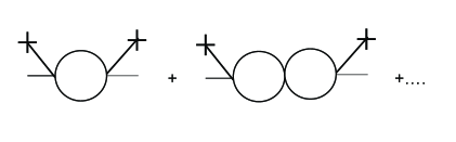
Figure 1: Feynman diagrams for the corrections to the two-point vertex function obtained by HFB approximation.

By using the homogeneous and static condition in Eq.(30) and applying the Fourier transformation in Eq.(31), we rewrite Eq.(73) as

$$\Gamma_{11}(k) = \upsilon^{2}+G_{11}^{tr}+\upsilon\Lambda_{221}^{tr}(k)+2\upsilon\Lambda_{121}^{tr}(k),$$

$$\Gamma_{22}(k) = \upsilon^{2}+G_{11}^{tr}+\upsilon\Lambda_{112}^{tr}(k)+2\upsilon\Lambda_{122}^{tr}(k),$$

$$\Gamma_{12}(k) = -i\omega+\mathbf{k}^{2}+\upsilon^{2}-G_{11}^{tr}+\upsilon\Lambda_{222}^{tr}(k)+2\upsilon\Lambda_{122}^{tr}(k),$$

$$\Gamma_{21}(k) = i\omega+\mathbf{k}^{2}+\upsilon^{2}-G_{11}^{tr}+\upsilon\Lambda_{111}^{tr}(k)+2\upsilon\Lambda_{121}^{tr}(k).$$ (75)

$\upsilon^{2}$ and $G_{ij}^{tr}$ in the above equation are obtained from the HFB equations in the previous section as in the end we take $J_{i}(x)=0$.

We start to calculate $\Lambda_{mnl}^{tr}(x,y)$. First, we differentiate Eq.(71) with respect to $\varphi_{m}(z)$,

$$\Gamma_{111}^{tr}(x,y,z) = \delta(x-y)\Lambda_{221}^{tr}(x,x,z),$$

$$\Gamma_{221}^{tr}(x,y,z) = \delta(x-y)\left(\Lambda_{111}^{tr}(x,x,z)+2\varphi_{1}\delta(x-z)\right),$$

$$\Gamma_{121}^{tr}(x,y,z) = \delta(x-y)\left(2\Lambda_{121}^{tr}(x,x,z)+2\varphi_{2}\delta(x-z)\right),$$

$$\Gamma_{211}^{tr}(x,y,z) = \delta(x-y)\left(2\Lambda_{121}^{tr}(x,x,z)+2\varphi_{2}\delta(x-z)\right),$$

$$\Gamma_{222}^{tr}(x,y,z) = \delta(x-y)\Lambda_{112}^{tr}(x,x,z),$$

$$\Gamma_{112}^{tr}(x,y,z) = \delta(x-y)\left(\Lambda_{222}^{tr}(x,x,z)+2\varphi_{2}\delta(x-z)\right),$$

$$\Gamma_{122}^{tr}(x,y,z) = \delta(x-y)\left(2\Lambda_{122}^{tr}(x,x,z)+2\varphi_{1}\delta(x-z)\right),$$

$$\Gamma_{212}^{tr}(x,y,z) = \delta(x-y)\left(2\Lambda_{122}^{tr}(x,x,z)+2\varphi_{1}\delta(x-z)\right),$$ (76)

where $z\equiv(\mathbf{z},\tau^{\prime\prime})$. From Eq.(14) we know

$$G_{mn}^{tr}(x,y)=\sum_{m^{\prime}}\sum_{n^{\prime}}\int dx^{\prime}\int dy^{\prime}G_{mm^{\prime}}^{tr}(x,x^{\prime})\Gamma_{m^{\prime}n^{\prime}}^{tr}(x^{\prime},y^{\prime})G_{n^{\prime}n}^{tr}(y^{\prime},y).$$ (77)

The derivatives of the above equation with respect to $\varphi_{l}(z)$ result in

$$\Lambda_{mnl}^{tr}(x,y,z)=-\sum_{m^{\prime}}\sum_{n^{\prime}}\int dx^{\prime}\int dy^{\prime}G_{mm^{\prime}}^{tr}(x,x^{\prime})\Gamma_{m^{\prime}n^{\prime}l}^{tr}(x^{\prime},y^{\prime},z)G_{n^{\prime}n}^{tr}(y^{\prime},y).$$ (78)

One can now take $J_{i}(x)=0$. $G_{mm^{\prime}}^{tr}(x,x^{\prime})$ is thus given by HFB approximation in the above equation. By substituting Eq.(76) into Eq.(78) and setting $x=y$, one obtains a set of closed equations for $\Lambda_{mnl}(x,x,z)$,

$$\Lambda_{mnl}(x,x,z)=-2\upsilon\left[G_{ml}^{tr}(x,z)G_{\bar{l}n}^{tr}(z,x)+G_{m\bar{l}}^{tr}(x,z)G_{ln}^{tr}(z,x)+G_{m\bar{l}}^{tr}(x,z)G_{\bar{l}n}^{tr}(z,x)\right]$$

$$-2\int dx^{\prime}\left(G_{ml}^{tr}(x,x^{\prime})G_{\bar{l}n}^{tr}(x^{\prime},x)\Lambda_{\bar{l}ll}(x^{\prime},x^{\prime},z)+G_{m\bar{l}}^{tr}(x,x^{\prime})G_{ln}^{tr}(x^{\prime},x)\Lambda_{\bar{l}ll}(x^{\prime},x^{\prime},z)\right)$$

$$-\int dx^{\prime}\left(G_{ml}^{tr}(x,x^{\prime})G_{ln}^{tr}(x^{\prime},x)\Lambda_{\bar{l}\bar{l}l}(x^{\prime},x^{\prime},z)+G_{m\bar{l}}^{tr}(x,x^{\prime})G_{\bar{l}n}^{tr}(x^{\prime},x)\Lambda_{lll}(x^{\prime},x^{\prime},z)\right),$$ (79)

where $\bar{l}$ is defined by $\delta_{l\bar{l}}=0$, which means $l=1$, $\bar{l}=2$ or $l=2$, $\bar{l}=1$. By applying the Fourier transformations in Eq.(31) we rewrite Eq. (79) as

$$\Lambda_{mnl}^{tr}(k) = \Lambda_{lll}^{tr}(k)I_{m\bar{l},\bar{l}n}(k)+\Lambda_{\bar{l}\bar{l}l}^{tr}(k)I_{ml,ln}(k)+\Lambda_{\bar{l}ll}^{tr}(k)\left(2I_{ml,\bar{l}n}(k)+2I_{m\bar{l},ln}(k)\right)$$ (80)

$$+2\upsilon\left(I_{ml,\bar{l}n}(k)+I_{m\bar{l},ln}(k)+I_{m\bar{l},\bar{l}n}(k)\right),$$

where

$$I_{mn,m^{\prime}n^{\prime}}(k)=-\int\frac{d\omega_{1}}{2\pi}\int\frac{d^{D}\mathbf{k}_{1}}{(2\pi)^{D}}G_{mn}^{tr}(k_{1}+k)G_{m^{\prime}n^{\prime}}^{tr}(k_{1})$$ (81)

and the two-point functions $G_{mn}^{tr}(k)$ are those obtained from the HFB equations. We can explicitly integrate $\omega_{1}$ in Eq.(81), for example,

$$I_{11,11}(k)=\frac{1}{4}\int\frac{d^{D}\mathbf{k}_{1}}{(2\pi)^{D}}\frac{-(\upsilon^{2}+G_{11}^{tr})^{2}}{\sqrt{\left((k+\mathbf{k}_{1})^{2}+2\upsilon^{2}\right)\left((k+\mathbf{k}_{1})^{2}-2G_{11}^{tr}\right)(\mathbf{k}_{1}^{2}+2\upsilon^{2})(\mathbf{k}_{1}^{2}-2G_{11}^{tr})}}$$

$$\times(\frac{1}{i\omega+\sqrt{\left((k+\mathbf{k}_{1})^{2}+2\upsilon^{2}\right)\left((k+\mathbf{k}_{1})^{2}-2G_{11}^{tr}\right)}+\sqrt{(\mathbf{k}_{1}^{2}+2\upsilon^{2})(\mathbf{k}_{1}^{2}-2G_{11}^{tr})}}$$

$$-\frac{1}{i\omega-\sqrt{\left((k+\mathbf{k}_{1})^{2}+2\upsilon^{2}\right)\left((k+\mathbf{k}_{1})^{2}-2G_{11}^{tr}\right)}-\sqrt{(\mathbf{k}_{1}^{2}+2\upsilon^{2})(\mathbf{k}_{1}^{2}-2G_{11}^{tr})}}),$$ (82)

which shall be used for analytic continuation described below. Next, we insert the $\Lambda_{mnl}(k)$ solved from Eq.(80) into Eq.(75), so as to obtain the improved two-point vertices $\Gamma_{mn}(k)$. The improved two-point correlation functions take the form

$$G_{12}(k) = \frac{1}{M(k)}\left[i\omega-\left(\mathbf{k}^{2}+\upsilon^{2}-G_{11}^{tr}+\upsilon\left(\Lambda_{222}^{tr}(k)+2\Lambda_{122}^{tr}(k)\right)\right)\right],$$

$$G_{22}(k) = \frac{1}{M(k)}\left[\upsilon^{2}+G_{11}^{tr}+\upsilon\left(\Lambda_{221}^{tr}(k)+2\Lambda_{121}^{tr}(k)\right)\right],$$

$$G_{11}(k) = \frac{1}{M(k)}\left[\upsilon^{2}+G_{11}^{tr}+\upsilon\left(\Lambda_{112}^{tr}(k)+2\Lambda_{122}^{tr}(k)\right)\right],$$

$$G_{21}(k) = \frac{1}{M(k)}\left[-i\omega-\left(\mathbf{k}^{2}+\upsilon^{2}-G_{11}^{tr}+\upsilon\left(\Lambda_{111}^{tr}(k)+2\Lambda_{121}^{tr}(k)\right)\right)\right],$$ (83)

where $M(k)$ is the determinant of the matrix $\Gamma_{mn}(k)$ and reads

$$M(k)=\left[\upsilon^{2}+G_{22}^{tr}+\upsilon\left(\Lambda_{221}^{tr}(k)+2\Lambda_{121}^{tr}(k)\right)\right]$$

$$\times\left[\upsilon^{2}+G_{11}^{tr}+\upsilon\left(\Lambda_{112}^{tr}(k)+2\Lambda_{122}^{tr}(k)\right)\right]$$

$$-\left[-i\omega-\mu+\mathbf{k}^{2}+2\upsilon^{2}+2G_{12}^{tr}+\upsilon\left(\Lambda_{222}^{tr}(k)+2\Lambda_{122}^{tr}(k)\right)\right]$$

$$\times\left[i\omega-\mu+\mathbf{k}^{2}+2\upsilon^{2}+2G_{12}^{tr}+\upsilon\left(\Lambda_{111}^{tr}(k)+2\Lambda_{121}^{tr}(k)\right)\right].$$ (84)

The Green function in Eq. (83) gives a gapless excitation spectrum, which shall be shown by the numerical result and also can be analytically verified by investigating the poles of the Green’s function. Analytically, one can prove $M(0)=0$ to make sure that the excitation spectrum is gapless. The details of the proof are put in the Appendix.

One can obtain the real time Green’s function, retarded and advanced Green’s function by analytic continuation, $i\omega\rightarrow\Omega\pm i\eta$, where $\eta$ is an infinitesimal positive number. The spectral weight function is then obtained by using the relation Fetter

$$\rho\left(\mathbf{k},\Omega\right)=2\text{Im}G^{A}\left(\mathbf{k},\Omega\right)=-2\text{Im}G^{R}\left(\mathbf{k},\Omega\right).$$ (85)

Eq. (82) is an analytic function of ”complex” variable $\Omega$ except on the real axis in $\Omega$ plane. The retarded and advanced Green’s function obtained therefore have desirable analytic properties.

There is an equivalent formalism of the IGA approximation in the framework of the improved $\Phi$ derivable theory. The $\Phi$ derivable theory can start with the two particle irreducible (2PI) action functional $\widetilde{\Gamma}\left[\varphi_{1},\varphi_{2},\mathbf{G}\right]$ which takes the form

$$\widetilde{\Gamma}\left[\varphi_{1},\varphi_{2},\mathbf{G}\right] = S\left[\varphi_{1},\varphi_{2}\right]+\frac{1}{2}Tr\ln\mathbf{G}^{-1}+\frac{1}{2}Tr\left[\mathbf{D}^{-1}\left(\mathbf{G}-\mathbf{D}\right)\right]+\Phi\left[\varphi_{1},\varphi_{2},\mathbf{G}\right]$$ (86)

$$\left(\mathbf{D}^{-1}\right)_{ij} = \frac{\delta^{2}S\left[\varphi_{1},\varphi_{2}\right]}{\delta\varphi_{i}\delta\varphi_{j}},$$

where $(\varphi_{1},\varphi_{2})\equiv(\varphi^{\ast},\varphi)$ as defined previously, and $\mathbf{G}$ represents matrix $\left(\mathbf{G}\right)_{ij}=G_{ij}$ of Green’s functions. In the order of HFB approximation (omitting higher order diagrams like the setting sun diagram),

$$\Phi\left[\varphi_{1},\varphi_{2},\mathbf{G}\right]=\frac{1}{2}\int dx\left[G_{11}\left(x,x\right)G_{22}\left(x,x\right)+2G_{12}\left(x,x\right)G_{21}\left(x,x\right)\right]$$ (87)

We will obtain the same equations as Eq.(44) and Eq.(45) of the HFB approximation if we require

$$\frac{\delta\widetilde{\Gamma}\left[\varphi_{1},\varphi_{2},\mathbf{G}\right]}{\delta\varphi_{i}}=0,\frac{\delta\widetilde{\Gamma}\left[\varphi_{1},\varphi_{2},\mathbf{G}\right]}{\delta G_{ij}}=0.$$ (88)

In the framework of the $\Phi$ derivable theory, IGA can be reformulated as below Ref.Hendrik . The 1PI effective action $\Gamma\left[\varphi_{1},\varphi_{2}\right]$ is equal to $\widetilde{\Gamma}\left[\varphi_{1},\varphi_{2},\mathbf{G}^{tr}\left(\varphi_{1},\varphi_{2}\right)\right]$ with $\mathbf{G}^{tr}\left(\varphi_{1},\varphi_{2}\right)$ defined by $\frac{\delta\widetilde{\Gamma}\left[\varphi_{1},\varphi_{2},\mathbf{G}\right]}{\delta G_{ij}}|_{\mathbf{G}=\mathbf{G}^{tr}\left(\varphi_{1},\varphi_{2}\right)}=0$. Then from $\Gamma\left[\varphi_{1},\varphi_{2}\right]$, one obtains the inverse Green’s function $\Gamma_{ij}=\frac{\delta^{2}\Gamma\left[\varphi_{1},\varphi_{2}\right]}{\delta\varphi_{i}\delta\varphi_{j}}=\frac{\delta^{2}\widetilde{\Gamma}\left[\varphi_{1},\varphi_{2},\mathbf{G}^{tr}\left(\varphi_{1},\varphi_{2}\right)\right]}{\delta\varphi_{i}\delta\varphi_{j}}$. For technical details, see Ref.Hendrik . Substituting the solution of Eq.(88) to the functional $\widetilde{\Gamma}\left[\varphi_{1},\varphi_{2},\mathbf{G}\right]$, we obtain a quantity $\Gamma$. The thermodynamical potential is $\beta^{-1}\Gamma$. According to the thermodynamical relation, the particle number density $n$ is equal to $-\frac{\partial\Gamma}{\beta L\partial\mu}$ with $L$ being the size of the 1D system( $L$ is infinity in the thermodynamic limit). Using Eq.(88) and Eq.(86), we know the density $n$ is equal to $\upsilon^{2}+G_{12}^{tr}$, the same as the case of HFB. It is also valid in any $\Phi$ derivable theory or improved $\Phi$ derivable theory beyond HFB.

V Comparison with the Exact Solution

The references key-19 ; key-29 present an exact solution of the Lieb-Liniger model, which gives the exact excitation spectrum.

The references key-19 ; key-29 consider a one-dimensional system of length $L$ (satisfying periodic boundary conditions), with $N$ bosonic particles interacting via a repulsive contact potential of strength $2c$, governed by the Lieb-Liniger Hamiltonian

$$H=-\sum_{i=1}^{N}\left(\partial^{2}/\partial x_{i}^{2}\right)+2c\sum_{1\leq i<j\leq N}\delta(x_{i}-x_{j}).$$ (89)

The excitation spectrum is plotted as $\omega/n^{2}\sim k/n$ , with $n$ being the particle number density $\frac{N}{L}$. The dimensionless parameter of the system is defined by $\gamma=\frac{c}{n}$. Comparing Eq.(18) with Eq.(89), there is $g=2c$ and hence the corresponding parameter in the field-theoretic treatment takes the form $\gamma=\frac{g}{2n}$.Comparing Eqs.(21)(23), we know $n=gn^{\prime}$, $\mathbf{k}=g\mathbf{k}^{\prime}$ and $\omega=g^{2}\omega^{\prime}$, which implies $\omega/n^{2}=\omega^{\prime}/n^{\prime 2}$, $\mathbf{k}/n=\mathbf{k}^{\prime}/n^{\prime}$, where we restore the notation $\mathbf{k}^{\prime}$, $n^{\prime}$, $\omega^{\prime}$ for the rescaled quantities after Eq.(23) (we had dropped prime for simplicity). Therefore, in order to compare with the exact solution, we should plot the excitation spectrum in the form $\omega^{\prime}/n^{\prime 2}\sim k^{\prime}/n^{\prime}$ with $n^{\prime}$ being the rescaled particle number density, at the parameter $\gamma=\frac{1}{2n^{\prime}}$. At the parameters $\gamma=1$, $\gamma=32$, $\gamma=64$, corresponding to $n^{\prime}=1/2$, $n^{\prime}=1/64$, $n^{\prime}=1/128$, we plot the spectrum obtained from the different approximation schemes in Fig. 2.  The IGA spectrum, which incorporates extra corrections based on the HFB spectrum, is gapless, while the HFB spectrum is gapped. When the particle density is high ($\gamma$ is small) , all approximation schemes lead to good results, which implies that quantum fluctuations are weak at a high particle density. Furthermore, at a very low particle density when quantum fluctuations become strong, the IGA scheme shows its advantage. Specifically, at $\gamma=32$ and $\gamma=64$, the IGA spectrum is in good agreement with the exact one, while the Bogoliubov spectrum is not accurate quantitatively.

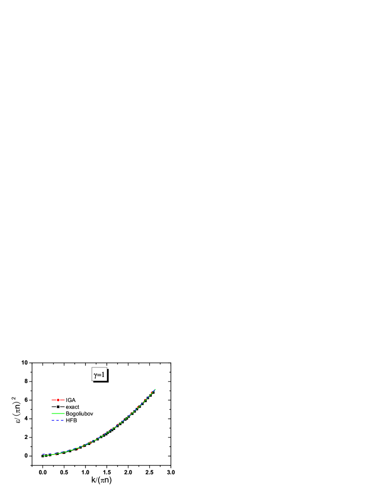
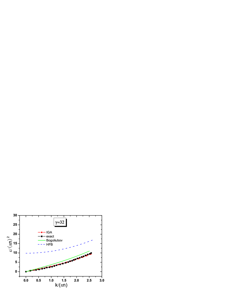
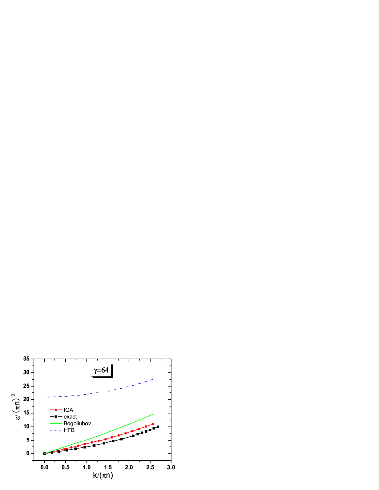
Figure 2: (color online)The spectra obtained from Bogoliubov approximation (green lines), HFB (blue dashed lines), IGA (red dotted lines) and exact numerical calculations (black squares) from Bethe ansatz key-29 are compared at three different $\gamma$.

VI Summary

We have presented IGA (improved Gaussian approximation) to treat one dimensional bosonic gas. The Green’s function obtained by IGA satisfies Ward identities from $U(1)$ symmetry and therefore the spectrum is gapless.

We have formulated all the traditional approximations (Bogoliubov approximation, HFB approximation and Popov approximation) in terms of truncations of Dyson-Schwinger equations. The HFB approximation is the well-known self-consistent approximation, but it leads to a gapped excitation spectrum, violating the Goldstone theorem. The spectrum obtained by IGA scheme, which incorporates more quantum corrections to the HFB spectrum, is gapless. In order to test the validity and precision of the IGA method, we apply it to the one-dimensional bosonic gas described by the Lieb-Liniger model. We can only obtain Type I excitation ( Bogoliubov spectrum) within IGA method. Nevertheless, by comparison with the type I spectrum exactly solved by the Bethe ansatz, we find that the IGA method gives quantitatively good results on type I spectrum.

The idea of the IGA method can be applied to improve higher order $\Phi$ derivable theory (the HFB theory is the result of the lowest order $\Phi$ derivable approximation) Hendrik ; Rosenstein . The essence of the idea is to add extra Feynman diagrams to preserve the symmetry of all the Feynman diagrams, and thereby restore the Ward identity. The IGA method makes improvement based on the HFB approximation. When quantum fluctuations are very strong, higher order $\Phi$ derivable approximation beyond the HFB approximation will be required and then the corresponding improvement to restore the Ward identity can be performed in a similar way. In order to get type II (Fermionic excitation), one probably shall go beyond IGA and use ”improved” high order $\Phi$ derivable theory.

The IGA method presented here can be employed to handle many other Bose-condensed systems, including 2D or 3D, zero temperature or finite temperature, homogeneous or in optical lattices. For higher dimension systems, as there is no type II excitation and quantum fluctuations are weaker, IGA shall be expected to give more quantitatively accurate results.

As one of applications of IGA, we have carried out the IGA calculation on type II superconductor where acoustic and optical spectra are obtained non-perturbatively. The results will be presented elsewhere In preparation .

VII Appendix

We shall prove $M(0)=0$, namely,

$$0 = \left[\upsilon^{2}+G_{22}^{tr}+\upsilon\left(\Lambda_{221}^{tr}(0)+2\Lambda_{121}^{tr}(0)\right)\right]$$ (90)

$$\times\left[\upsilon^{2}+G_{11}^{tr}+\upsilon\left(\Lambda_{112}^{tr}(0)+2\Lambda_{122}^{tr}(0)\right)\right]$$

$$-\left[-\mu+2\upsilon^{2}+2G_{12}^{tr}+\upsilon\left(\Lambda_{222}^{tr}(0)+2\Lambda_{122}^{tr}(0)\right)\right]$$

$$\times\left[-\mu+2\upsilon^{2}+2G_{12}^{tr}+\upsilon\left(\Lambda_{111}^{tr}(0)+2\Lambda_{121}^{tr}(0)\right)\right].$$

By using the homogeneous and static condition in Eq.(30) and applying the Fourier transformation in Eq.(31), we rewrite Eq.(70) as

$$0 = -\mu+\upsilon^{2}+G_{11}^{tr}+2G_{12}^{tr},$$

$$G_{11}^{tr} = G_{22}^{tr},$$ (91)

and Eq.(71) as

$$\Gamma_{11}^{tr}(k) = \upsilon^{2}+G_{11}^{tr},$$

$$\Gamma_{22}^{tr}(k) = \upsilon^{2}+G_{11}^{tr},$$

$$\Gamma_{12}^{tr}(k) = -i\omega+\mathbf{k}^{2}+\upsilon^{2}-G_{11}^{tr},$$

$$\Gamma_{21}^{tr}(k) = i\omega+\mathbf{k}^{2}+\upsilon^{2}-G_{11}^{tr}.$$ (92)

Note that the value of the external sources $J_{1}$ and $J_{2}$ has been set to zero. With the help of Eq.(32) we obtain the two-point truncated Green’s function,

$$\left(\begin{array}[]{cc}G_{11}^{tr}(k)&G_{12}^{tr}(k)\\ G_{21}^{tr}(k)&G_{22}^{tr}(k)\end{array}\right) = \frac{1}{(i\omega)^{2}-\left(\mathbf{k}^{2}+2\upsilon^{2}\right)\left(\mathbf{k}^{2}-2G_{11}^{tr}\right)}$$ (98)

$$\times\left(\begin{array}[]{cc}\upsilon^{2}+G_{11}^{tr}&i\omega-\left(\mathbf{k}^{2}+\upsilon^{2}-G_{11}^{tr}\right)\\ -i\omega-\left(\mathbf{k}^{2}+\upsilon^{2}-G_{11}^{tr}\right)&\upsilon^{2}+G_{11}^{tr}\end{array}\right),$$

which has the same form as the Green’s function in the HFB approximation. Using Eq.(91) we can rewrite Eq.(90) as

$$0 = \left[\upsilon^{2}+G_{11}^{tr}+\upsilon\left(\Lambda_{221}^{tr}(0)+2\Lambda_{121}^{tr}(0)\right)\right]$$ (99)

$$\times\left[\upsilon^{2}+G_{11}^{tr}+\upsilon\left(\Lambda_{112}^{tr}(0)+2\Lambda_{122}^{tr}(0)\right)\right]$$

$$-\left[\upsilon^{2}-G_{11}^{tr}+\upsilon\left(\Lambda_{222}^{tr}(0)+2\Lambda_{122}^{tr}(0)\right)\right]$$

$$\times\left[\upsilon^{2}-G_{11}^{tr}+\upsilon\left(\Lambda_{111}^{tr}(0)+2\Lambda_{121}^{tr}(0)\right)\right].$$

By inserting Eq.(98) in Eq.(81), it is easy to verify that

$$I_{ml,ln}(0)=I_{\bar{m}\bar{l},\bar{l}\bar{n}}(0)\,,$$ (100)

where $m,n,l,\bar{m},\bar{n},\bar{l}=1,2$ with the constraint $\delta_{m\bar{m}}=0$, $\delta_{n\bar{n}}=0$ and $\delta_{l\bar{l}}=0$. For example, $I_{11,11}(0)=I_{22,22}(0)$, $I_{21,11}(0)=I_{12,22}(0)$, etc. Eq.(100) and Eq.(80) lead to

$$\Lambda_{mnl}^{tr}(0)\equiv\Lambda_{\bar{m}\bar{n}\bar{l}}^{tr}(0)\,.$$ (101)

There is

$$\Lambda_{mnl}^{tr}(k)=\Lambda_{nml}^{tr}(k)\,,$$ (102)

which is evident from the definition in Eq.(74). Using Eq.(101)and Eq.(102) we can rewrite Eq.(99) as

$$0 = \left(2\upsilon+4\Lambda_{121}^{tr}(0)+\Lambda_{111}^{tr}(0)+\Lambda_{221}^{tr}(0)\right)$$ (103)

$$\times\left(2G_{11}^{tr}+\upsilon\Lambda_{221}^{tr}(0)-\upsilon\Lambda_{111}^{tr}(0)\right).$$

From Eq.(80) we find that

$$\left(\Lambda_{221}^{tr}(0)-\Lambda_{111}^{tr}(0)\right)=\frac{2\upsilon\left(I_{11,11}(0)-I_{12,21}(0)\right)}{\left(1+I_{11,11}(0)-I_{12,21}(0)\right)}\,.$$ (104)

By straightforward calculations, we know

$$I_{11,11}(0)-I_{12,21}(0)=\frac{1}{4\pi}\int_{0}^{\infty}dk\frac{1}{\sqrt{\left(k^{2}+2\upsilon^{2}\right)\left(k^{2}-2G_{11}^{tr}\right)}}\,,$$ (105)

and

$$G_{11}^{tr}=-\left(\upsilon^{2}+G_{11}^{tr}\right)\frac{1}{4\pi}\int_{0}^{\infty}dk\frac{1}{\sqrt{\left(k^{2}+2\upsilon^{2}\right)\left(k^{2}-2G_{11}^{tr}\right)}}.$$ (106)

Eq.(106) follows from the definition of $G_{11}^{tr}$, that is $G_{11}^{tr}=G_{11}^{tr}(x,x)=\int\frac{d\omega}{2\pi}\int\frac{d^{D}\mathbf{k}}{(2\pi)^{D}}G_{11}^{tr}(\mathbf{k},\omega)$. By comparing Eq.(105) and Eq.(106) we know

$$I_{11,11}(0)-I_{12,21}(0)=\frac{-G_{11}^{tr}}{\left(\upsilon^{2}+G_{11}^{tr}\right)}\,.$$ (107)

Eq.(104) and Eq.(107) lead to

$$2G_{11}^{tr}+\upsilon\Lambda_{221}^{tr}(0)-\upsilon\Lambda_{111}^{tr}(0)=0.$$ (108)

Thus Eq.(103) is proved and also Eq.(90) is proved.

References

(1) N. N. Bogoliubov, J. Phys. (Moscow) 11, 23 (1947).
(2) N. N. Bogoliubov, Moscow Univ. Phys. Bull. 7, 43 (1947).
(3) N. N. Bogoliubov, Lectures on Quantum Statistics
(Gordon and Breach, New York, 1967),Vol.1.
(4) N. N. Bogoliubov, Lectures on Quantum Statistics
(Gordon and Breach, New York, 1970),Vol.2.
(5) S.T. Beliaev, J. Exp. Theor. Phys. 7, 289 (1958).
(6) S.T. Beliaev, J. Exp. Theor. Phys. 7, 299 (1958).
(7) N. M. Hugenholtz and D. Pines, Phys. Rev. 116, 489
(1959).
(8) J. Goldstone, Nuovo Cimento 19, 154 (1961).
(9) P. C. Hohenberg and P. C. Martin, Ann. Phys. 34,
291 (1965).
(10) J. Luttinger and J. Ward, Phys. Rev. 118, 1417
(1960).
(11) C. de Dominicis and P.C. Martin, J. Math. Phys. 5,
14 (1964).
(12) C. de Dominicis and P.C. Martin, J. Math. Phys. 5,
31 (1964).
(13) J. M. Cornwall, R. Jackiw, and E. Tom boulis, Phys. Rev. D
10, 2428 (1974).
(14) G. Baym and Leo P. Kadanoff , Phys. Rev. 124, 287
(1961). G. Baym, Phys. Rev. 127, 1391 (1962).
(15) A. Griffin, Phys. Rev. B 53, 9341 (1996).
(16) H. Shi and A. Griffin, Phys. Rep. 304, 1 (1998).
(17) D. A. W. Hutchinson et al., J. Phys. B 33, 3825 (2000).
(18) V. N. Popov, Functional Integrals in Quantum Field
Theory and Statistical Physics (Reidel, Dordrecht, 1983).
(19) E. Lundh and J. Rammer, Phys. Rev. A 66, 033607
(2002).
(20) J. O. Andersen, Rev. Mod. Phys. 76, 599 (2004).
(21) H. van Hees and J. Knoll, Phys. Rev. D 66, 025028
(2002).
(22) A. Kovner and B. Rosenstein, Phys. Rev. D 39,
2332 (1989). B. Rosenstein and A. Kovner, Phys. Rev. D 40, 504
(1989).
(23) A. Okopińska, Physics Letters B, 375, 213
(1996). A. Okopińska, arXiv:cond-mat/0309679v1.
(24) A. Görlitz et al., Phys. Rev. Lett. 87, 130402 (2001).
(25) H. Moritz, T. Stöferle, M. Köhl, and T. Esslinger,
Phys. Rev. Lett. 91, 250402 (2003).
(26) B. Paredes et al., Nature (London) 429,
277 (2004).
(27) T. Kinoshita, T. Wenger, and D. S. Weiss, Science 305, 1125 (2004).
(28) D.S. Petrov, G.V. Shlyapnikov, and J.T.M.
Walraven, Phys. Rev. Lett. 85, 3745 (2000).
(29) D.M. Gangardt and G.V. Shlyapnikov, Phys. Rev.
Lett. 90, 010401 (2003).
(30) M. A. Cazalilla et al., Rev. Mod. Phys. 83, 1405 (2011), references therein.
(31) E. Lieb, Phys. Rev. 130, 1616 (1963).
(32) E. Lieb and W. Liniger, Phys. Rev. 130, 1605
(1963).
(33) M. Olshanii, Phys. Rev. Lett. 81, 938 (1998).
(34) V. Dunjko, V. Lorent, and M. Olshanii, Phys. Rev. Lett.
86, 5413 (2001).
(35) J. S. Caux, P. Calabrese and N. A. Slavnov, Journal of
Statistical Mechanics: Theory and Experiment 2007, P01008 (2007);
J. S. Caux and P. Calabrese, Phys. Rev. A 74, 031605(R) (2006).
(36) Algebraic Bethe Ansatz Computation of Universal Structure
factors. See http://staff.science.uva.nl/jcaux/ABACUS.html.
(37) J. W. Negele and H. Orland, Quantum Many-Particle
Systems (Westview Press, 1988).
(38) R. Jackiw, Phys. Rev. D 9, 1686 (1974).
(39) J.O. Andersen, U. Al Khawaja, and H.T.C. Stoof, Phys. Rev.
Lett. 88, 070407 (2002);U. Al Khawaja, J.O. Andersen, N.P.
Proukakis, and H.T.C Stoof, Phys. Rev. A66 013615 (2002).
(40) E. Calzetta and B. L. Hu, Nonequilibrium quantum
field theory, Chap.13 (Cambridge University Press, 2008).
(41) A. L. Fetter and J. D. Walecka, Quantum Theory of
Many Particle Systems (McGraw-Hill, New York, 1971).
(42) Qiong Li, Li Zhang and Dingping Li, in
preparation.