Invasions in heterogeneous habitats in the presence of advection

Abstract

We investigate invasions from a biological reservoir to an initially empty, heterogeneous habitat in the presence of advection. The habitat consists of a periodic alternation of favorable and unfavorable patches. In the latter the population dies at fixed rate. In the former it grows either with the logistic or with an Allee effect type dynamics, where the population has to overcome a threshold to grow. We study the conditions for successful invasions and the speed of the invasion process, which is numerically and analytically investigated in several limits. Generically advection enhances the downstream invasion speed but decreases the population size of the invading species, and can even inhibit the invasion process. Remarkably, however, the rate of population increase, which quantifies the invasion efficiency, is maximized by an optimal advection velocity. In models with Allee effect, differently from the logistic case, above a critical unfavorable patch size the population localizes in a favorable patch, being unable to invade the habitat. However, we show that advection, when intense enough, may activate the invasion process.

1 Introduction

Invasions of alien species are widespread phenomena, in principle affecting every ecosystem, usually with dramatic consequences on the native community, constituting a major threat to biodiversity (Vitousek et al, 1997; Mooney, 2000; Pimentel et al, 2000). At the scale of interest for management purposes, i.e. the geographic scale, invasive species move across a heterogeneous landscape characterized by favorable and unfavorable areas. The presence of abiotic heterogeneity, in fact, characterizes most of natural habitats and plays a key role in invasion processes, influencing their rate of spread and outcome (Shigesada and Kawasaki, 1997; Hastings et al, 2005; Melbourne et al., 2007).

Alongside with the empirical interest for the problem, several modeling efforts have been dedicated to the understanding and prediction of the spatial spread of invading organisms in heterogeneous environments. Within the framework of reaction diffusion models, building on the pioneering theoretical works of Skellam (1951) and Kierstead and Slobodkin (1953) on the “critical patch size” problem, Shigesada et al (1986) gave a seminal contribution considering the invasion (propagation) of a population through a periodic heterogeneous environment (see also Weinberger, 2002; Kinezaki et al, 2003). The problem was extended including advective transport to study persistence and propagation of passively dispersing populations in oceans (Mann and Lazier, 1991; Abraham, 1998) or rivers (Speirs and Gurney, 2001; Pachepsky et al, 2005; Lutscher et al, 2006). The importance of the interplay between heterogeneity and advection has been recently reviewed by Ryabov and Blasius (2008). Moreover, the role of both advection and landscape spatial structure is clearly relevant also to the dispersal of plants (Hastings et al, 2005), whose seeds are transported by winds.

In this article, we focus on the interplay between abiotic heterogeneity and advection in invasions. We describe the dynamics in terms of an advection-reaction-diffusion model, which allows for mathematical tractability and quantitative predictions, e.g., on the spreading rates.

We consider an infinite system where a population stably saturates the carrying capacity on one side of the system and possibly invades the remaining part of the environment, which is assumed to be heterogeneous. Our setting is quite general and widely applicable. In particular, it is relevant to situations in which one has a practically infinite biological reservoir of a species invading an empty territory characterized by abiotic heterogeneity. For instance, the above setting may be relevant to situations in which invasions can suddenly become possible for the removal of a climatic barrier due to climate changes (Mooney, 2000). Another relevant case is when a species stably populating a lake invades an effluent characterized by a certain degree of heterogeneity and stream velocity. This is one of the key early-stage processes related to the spatial control of invasions in lakes’ networks (Havel et al, 2002). Other examples concern the spreading of wind-pollinated plants in a heterogeneous environment (Davis et al, 2004) or spores carried by the wind (Kot et al, 1996).

More specifically, the habitat consists of a periodic alternation of unfavorable and favorable patches, as in Shigesada et al (1986). The population dies at a fixed rate in unfavorable regions, and grows in favorable ones according to either a logistic or an Allee effect dynamics. We are interested in determining the conditions for invasions to be possible and in understanding how invasion speed and efficiency depend on the mechanisms at play.

With the logistic dynamics, in the absence of advection, this problem was pioneered by Shigesada et al (1986), while Lutscher et al (2006) considered both advection and heterogeneity in reference to the “drift paradox” problem (Speirs and Gurney, 2001). Going beyond these works, we find asymptotic expressions for both the invasion speed and the rate of increase of the population size. The latter quantity essentially estimates the rate at which the number of invading individuals grows and, thus, provides a suitable measure of the efficiency of the spreading process. Indeed, especially in invasive species control, it is important to quantify the potentiality of growth of an alien population, and not only the speed at which it colonizes the territory. We anticipate that, remarkably, larger invasion speeds do not necessarily imply more efficient invasions.

The logistic case (decreasing per capita growth rate) is then contrasted with the case of positive density dependence corresponding to a demographic Allee effect (Allee, 1938; Dennis, 1989), which accounts for a reduced reproductive power at low densities. The importance of Allee effects for the invasion and control of non-native species was emphasized by Taylor and Hastings (2005) and Tobin et al (2011). It is interesting to mention that even in homogeneous habitats the presence of the Allee effect can decrease the invasion speed or even halt the population spreading if the initially occupied area is too small (Lewis and Kareiva, 1993) (see also Vercken et al (2011) for recent field observations). We find that the interplay between heterogeneity and advection becomes very subtle in the presence of the Allee effect. In fact it may happen that a persisting population, unable to invade new territory, becomes able to spread in the presence of strong advection. This effect should be taken as a cautionary note from the standpoint of controlling invasive species, telling us that advective transport should be considered. For instance, after strong weather events, or in regions characterized by prevailing winds, neglecting the effects of advection could lead to the erroneous prediction of a population unable to invade, whereas it actually propagates over the territory.

The material is organized as follows. In Sect. 2 we present the model, and in Sect. 3 we qualitatively discuss its phenomenology. Sections 4 and 5 present and discuss the main results on invasions with the logistic and the Allee effect model, respectively. Finally, in Sect. 6 we summarize the results.

2 Model

The evolution of the population, $\theta(x,t)$, is governed by the advection-reaction-diffusion equation

$$\partial_{t}\theta+v\partial_{x}\theta=D\partial^{2}_{x}\theta+f(\theta,x)\,.$$ (1)

The diffusion coefficient $D$ and the advection velocity $v$ are assumed to be constant. Heterogeneity is introduced in the growth term, $f(\theta,x)$, which depends on the position $x$. The habitat consists of a periodic alternation of unfavorable and favorable patches of sizes $\ell_{u}$ and $\ell_{f}$, respectively. In the elementary cell $[0:\mathcal{L}]$ (where $\mathcal{L}=\ell_{u}+\ell_{f}$ denotes the spatial period), we take

$$f(\theta,x)=\left\{\begin{array}[]{ll}g_{u}(\theta)&\quad\;0\leq x<\ell_{u}\\ g_{f}(\theta)&\quad\;\ell_{u}\leq x<\mathcal{L}\end{array}\right.\,.$$ (2)

In the unfavorable regions the population is assumed to die at a constant rate $r_{u}$, so that $g_{u}(\theta)=-r_{u}\theta$ ($r_{u}>0$). In the favorable regions we consider two dynamics. The first is the classical logistic model (with carrying capacity normalized to one)

$$g_{f}(\theta)=r_{f}\theta(1-\theta)\,,$$ (3)

$r_{f}$ being the intrinsic growth rate. Equation (1) with the logistic term but without advection was firstly studied by Shigesada et al (1986). Recently, Lutscher et al (2006) included advection focusing on the “drift paradox” problem.

Secondly, accounting for a positive correlation between population density and per capita growth rate at small densities — the Allee effect (Allee, 1938; Dennis, 1989) —, we consider the threshold model

$$g_{f}(\theta)=r_{f}\max\{(\theta-\theta_{c})(1-\theta),0\}\,,$$ (4)

prescribing that the population grows only when $\theta>\theta_{c}$ (otherwise it stays constant). Notice that (4) recovers (3) for $\theta_{c}=0$. We remark that the model (4) represents an intermediate case between weak and strong Allee effect (Courchamp et al, 2008, see also Sect. 5 for further discussions). To the best of our knowledge, models with Allee effects have been mostly investigated in homogeneous habitats (Petrovskii and Li, 2003). In heterogeneous habitats we are aware of only a few studies with integro-difference models incorporating different dispersal kernels (see, e.g., the recent work by Dewhirst and Lutscher, 2009; Pachepsky and Levine, 2011).

We now specify the settings in which Eq. (1) is studied. We consider model (1) with boundary condition $\theta(0,t)=1$, mimicking the case in which on the left of the origin ($x<0$) the population constantly saturates the carrying capacity, while the population is initially absent in the $x>0$ region, i.e. $\theta(x,0)=0$ for $x>0$. With this choice for the boundary conditions the invasion process must be considered from left to right (i.e. from the biological reservoir at $x\leq 0$ to the positive real axis). In this case depending on the sign of the advection velocity we can consider (downstream) invasions with the flow (i.e when $v>0$) or (upstream) invasions against the flow (i.e. when $v<0$).

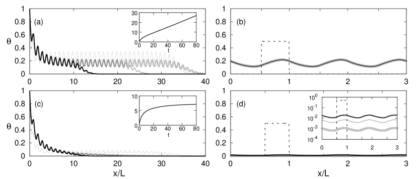
Figure 1: Population evolution with logistic dynamics and boundary condition (BC) $\theta(0,t)=1$ (a,c) or with periodic BC, $\theta(0,t)=\theta(nL,t)$ with $n=3$(b,d). Panel (a): Successful invasion for $l_{u}\!=\!2$, $l_{f}\!=\!1.8$, $\epsilon\!=\!1$ and $u=0.7$. The solid curves represent $\theta(x,t)$ at three successive times while the dotted curve corresponds to the case without advection ($u=0$), for comparison. The inset shows $\int_{0}^{\infty}dx\theta(x,t)$ vs $t$. Panel (b): Using the same parameters as in (a) but with periodic BC. The dashed rectangle corresponds to the initial condition, while the gray thick line is the population at stationarity. The black line superimposed on the gray one is obtained taking a cut of the interior of the traveling front from (a). Panel (c): Unsuccessful invasion obtained in the same settings as in (a) but for $l_{f}=1.4$, notice that here for $u=0$ the invasion is still possible, meaning that advection is responsible for the halt of the invasion process. The three solid curves refer to the same time instants of (a), while the dotted one is the $u=0$ case. Inset as in (a). Panel (d): parameters as in (c) but with periodic BC. Now the population goes extinct. The inset displays $\theta(x,t)$ at three successive times (from top to bottom) showing that $\theta\to 0$ exponentially.

It is useful to formulate the model in non-dimensional variables. To this aim we exploit known results about the logistic growth model without advection, namely for the standard FKPP equation (Fisher, 1937; Kolmogorov et al, 1937). The FKPP equation develops traveling fronts characterized by the propagation speed $v_{0}=2\mathchoice{{\hbox{$\displaystyle\sqrt{Dr_{f}\,}$}\lower 0.4pt\hbox{\vrule height=6.83331pt,depth=-5.46667pt}}}{{\hbox{$\textstyle\sqrt{Dr_{f}\,}$}\lower 0.4pt\hbox{\vrule height=6.83331pt,depth=-5.46667pt}}}{{\hbox{$\scriptstyle\sqrt{Dr_{f}\,}$}\lower 0.4pt\hbox{\vrule height=4.78333pt,depth=-3.82668pt}}}{{\hbox{$\scriptscriptstyle\sqrt{Dr_{f}\,}$}\lower 0.4pt\hbox{\vrule height=3.41666pt,depth=-2.73334pt}}}$ and width $\xi_{0}=\mathchoice{{\hbox{$\displaystyle\sqrt{D/r_{f}\,}$}\lower 0.4pt\hbox{\vrule height=7.5pt,depth=-6.00003pt}}}{{\hbox{$\textstyle\sqrt{D/r_{f}\,}$}\lower 0.4pt\hbox{\vrule height=7.5pt,depth=-6.00003pt}}}{{\hbox{$\scriptstyle\sqrt{D/r_{f}\,}$}\lower 0.4pt\hbox{\vrule height=5.25pt,depth=-4.20003pt}}}{{\hbox{$\scriptscriptstyle\sqrt{D/r_{f}\,}$}\lower 0.4pt\hbox{\vrule height=3.75pt,depth=-3.00002pt}}}$. It is then natural to measure lengths in units of $\xi_{0}$, time in units of the inverse growth rate in the favorable patches $1/r_{f}$, and the advection velocity in units of $v_{0}$. We thus define the non-dimensional variables $x^{\prime}=x/\xi_{0}$, $t^{\prime}=tr_{f}$, $u=v/v_{0}$. Dropping the primes, Eq. (1) made non-dimensional reads

$$\partial_{t}\theta+2u\partial_{x}\theta=\partial^{2}_{x}\theta+f(\theta,x)\,.$$ (5)

The factor $2$ in the advection term results from our choice to fix $u=1$ as the non-dimensional propagation speed in the homogeneous FKPP system. We can now introduce $\epsilon=r_{u}/r_{f}$ which is the death over growth rate ratio, and $l_{f,u}=\ell_{f,u}/\xi_{0}$ which are the non-dimensional sizes of the patches ($L=\mathcal{L}/\xi_{0}=l_{u}+l_{f}$). In this way, with reference to Eq. (2) we have $g_{u}(\theta)=-\epsilon\theta$ and

$$g_{f}(\theta)=\theta(1-\theta)\,,$$ (6)

for the logistic model, while with an Allee effect it becomes

$$g_{f}(\theta)=\max\left\{(\theta-\theta_{c})(1-\theta),0\right\}\,.$$ (7)

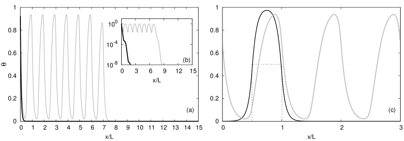
Figure 2: Population evolution with the Allee effect model (7). The black and gray curves are obtained without advection ($u=0$) and with advection ($u=0.5$), respectively. The other parameters are $\epsilon=1$, $l_{f}=l_{u}=8$ and $\theta_{c}=0.001$. The different panels refer to: (a) BC $\theta(0,t)=1$, (b) the same of (a) but in logarithmic scale, (c) periodic BC with $n=3$ elementary cells. The dashed line in (c) is the initial condition.

3 Model phenomenology

We now present the basic phenomenology of the model, discussing also the main differences between logistic and Allee effect growth models. A successful invasion implies the development, far from the boundary, of a traveling front, characterized by a stationary and spatially periodic bulk (Fig. 1a). In such a case the total population in the invaded habitat, $\int_{0}^{\infty}dx\theta(x,t)$, asymptotically increases linearly with time (inset of Fig. 1a). Faster growing populations mean more effective invasions. Conversely, Fig. 1c shows a typical case of unsuccessful invasion: no traveling front develops and the total population remains bounded in the limit of long times (compare the insets in Figs. 1a and 1c).

For positive advection velocities, the problem of identifying the conditions for successful invasions is directly related to determining under which conditions Eq. (5) with (6) in a finite system (of size $nL$ with $n$ integer) with periodic boundary conditions ($\theta(0,t)=\theta(nL,t)$) admits a non-vanishing stationary solution, starting from a generic non-zero initial condition. This is clearly shown by the perfect superposition of the bulk of the traveling front with the stationary solution of the periodic boundary condition problem (Fig. 1b). The reason for this link is that the bulk region of the traveling front (which is stationary and spatially periodic) satisfies the same boundary value problem of the finite system with periodic boundary conditions (BC). Therefore, to determine whether downstream invasions are successful it is enough to study whether persistence is possible in the finite system with periodic BC. Conversely, an unsuccessful invasion implies that in the finite system the population goes extinct, exponentially in time (inset of Fig.1d).

As we will see in the following, for small patch sizes, the qualitative behavior of the different growth models is very similar: invasions benefit from larger favorable regions and their speed increases accordingly; moreover, the presence of advection enhances the downstream invasion speed but decreases the population size of the invading species, eventually halting the invasion (see Fig.1). Conversely, for large enough unfavorable patches, dramatic differences appear. In the Allee effect model, the population can persist in the absence of advection but localized in a region of finite size, if it initially occupied that area (see Fig. 2c), being unable to invade new territories. This is quite different from the logistic model where invasions and persistence are always linked. Even more striking is the role of advection. Figures 2a,b show that suitable values of the advection velocity can activate the invasion of an otherwise localized population.

In the following we present the results for the logistic and Allee effect model separately as the level of analytical understanding is quite different. The possibility to use the linear analysis framework in the logistic model, indeed, allows us to systematically derive the conditions for invasions and asymptotic expressions for the invasion speed and efficiency. This approach cannot be used for the Allee effect model, which is studied mainly numerically and with heuristic arguments.

4 Results for the logistic growth model

4.1 Persistence in a closed periodic system

In this section we focus on the conditions for persistence in a closed system with periodic BC, which correspond to those for successful downstream invasion. Moreover, when the population is able to persist, we study how its size behaves as a function of the advection velocity. It is worth noticing that the closed system setting is interesting also in consideration of recent experiments where bacterial populations are grown in heterogeneous conditions (Dahmen et al, 2000; Lin et al, 2004; Perry, 2005).

4.1.1 Critical patch size and critical advection

Starting from a population different from zero in a single favorable patch, with periodic BC, Eq. (5) with (6) admits either the trivial solution $\theta=0$, meaning that the habitat is unable to sustain the population, or an asymptotically stationary non-vanishing solution, when persistence is possible. To determine the conditions for the latter, it is sufficient to identify when the solution $\theta=0$ becomes linearly unstable, as briefly sketched in A.

For $l_{u}$ and $\epsilon$ fixed it is possible to show the existence of both a critical size of the favorable patch, $l_{f}^{*}$, such that extinction occurs if $l_{f}\leq l_{f}^{*}$, and a critical advection velocity $u_{c}$ such that for a range of values of $l_{f}$ the system goes extinct if $u>u_{c}$. The implicit relation between the critical values reads

$$\begin{array}[]{l}{\cosh(uL)}\!-\!\cos(\mathchoice{{\hbox{$\displaystyle\sqrt{1-u^{2}\,}$}\lower 0.4pt\hbox{\vrule height=6.44444pt,depth=-5.15558pt}}}{{\hbox{$\textstyle\sqrt{1-u^{2}\,}$}\lower 0.4pt\hbox{\vrule height=6.44444pt,depth=-5.15558pt}}}{{\hbox{$\scriptstyle\sqrt{1-u^{2}\,}$}\lower 0.4pt\hbox{\vrule height=4.51111pt,depth=-3.6089pt}}}{{\hbox{$\scriptscriptstyle\sqrt{1-u^{2}\,}$}\lower 0.4pt\hbox{\vrule height=3.44165pt,depth=-2.75334pt}}}l_{f})\cosh(\mathchoice{{\hbox{$\displaystyle\sqrt{\epsilon+u^{2}\,}$}\lower 0.4pt\hbox{\vrule height=6.10999pt,depth=-4.88802pt}}}{{\hbox{$\textstyle\sqrt{\epsilon+u^{2}\,}$}\lower 0.4pt\hbox{\vrule height=6.10999pt,depth=-4.88802pt}}}{{\hbox{$\scriptstyle\sqrt{\epsilon+u^{2}\,}$}\lower 0.4pt\hbox{\vrule height=4.30276pt,depth=-3.44223pt}}}{{\hbox{$\scriptscriptstyle\sqrt{\epsilon+u^{2}\,}$}\lower 0.4pt\hbox{\vrule height=3.44165pt,depth=-2.75334pt}}}l_{u})=\\ \frac{\epsilon\!-\!1+2u^{2}}{2\mathchoice{{\hbox{$\displaystyle\sqrt{(1\!-\!u^{2})(\epsilon\!+\!u^{2})\,}$}\lower 0.4pt\hbox{\vrule height=5.25pt,depth=-4.20003pt}}}{{\hbox{$\textstyle\sqrt{(1\!-\!u^{2})(\epsilon\!+\!u^{2})\,}$}\lower 0.4pt\hbox{\vrule height=5.25pt,depth=-4.20003pt}}}{{\hbox{$\scriptstyle\sqrt{(1\!-\!u^{2})(\epsilon\!+\!u^{2})\,}$}\lower 0.4pt\hbox{\vrule height=3.67499pt,depth=-2.94pt}}}{{\hbox{$\scriptscriptstyle\sqrt{(1\!-\!u^{2})(\epsilon\!+\!u^{2})\,}$}\lower 0.4pt\hbox{\vrule height=2.625pt,depth=-2.10002pt}}}}\sin(\mathchoice{{\hbox{$\displaystyle\sqrt{1\!-\!u^{2}\,}$}\lower 0.4pt\hbox{\vrule height=6.44444pt,depth=-5.15558pt}}}{{\hbox{$\textstyle\sqrt{1\!-\!u^{2}\,}$}\lower 0.4pt\hbox{\vrule height=6.44444pt,depth=-5.15558pt}}}{{\hbox{$\scriptstyle\sqrt{1\!-\!u^{2}\,}$}\lower 0.4pt\hbox{\vrule height=4.51111pt,depth=-3.6089pt}}}{{\hbox{$\scriptscriptstyle\sqrt{1\!-\!u^{2}\,}$}\lower 0.4pt\hbox{\vrule height=3.44165pt,depth=-2.75334pt}}}l_{f})\sinh(\mathchoice{{\hbox{$\displaystyle\sqrt{\epsilon\!+\!u^{2}\,}$}\lower 0.4pt\hbox{\vrule height=6.10999pt,depth=-4.88802pt}}}{{\hbox{$\textstyle\sqrt{\epsilon\!+\!u^{2}\,}$}\lower 0.4pt\hbox{\vrule height=6.10999pt,depth=-4.88802pt}}}{{\hbox{$\scriptstyle\sqrt{\epsilon\!+\!u^{2}\,}$}\lower 0.4pt\hbox{\vrule height=4.30276pt,depth=-3.44223pt}}}{{\hbox{$\scriptscriptstyle\sqrt{\epsilon\!+\!u^{2}\,}$}\lower 0.4pt\hbox{\vrule height=3.44165pt,depth=-2.75334pt}}}l_{u})\end{array}.{}$$ (8)

The above equation was also found by Lutscher et al (2006) using boundary conditions different from ours. Notice that for $|u|>1$ the term $\textstyle\sqrt{1-u^{2}\,}$  becomes imaginary, and in Eq. (8) the identities $\sin(iz)=i\sinh(z)$ and $\tan(iz)=i\tanh(z)$ must be employed. We also remark that Eq. (8) is left unchanged by the substitution $u\to-u$ due to the symmetries of model (5) with periodic BC. Therefore, we can limit the analysis to $u\geq 0$.

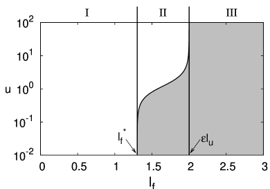
Figure 3: Extinction (white) and survival (gray) regions in the plane ($l_{f},u$). The boundary curve between the two regions gives the dependence of the critical velocity $u_{c}$ on $l_{f}$. The two vertical lines pinpoint the values $l_{f}^{*}$ and $\epsilon l_{u}$. The Roman numbers on top label the three regions discussed in the text. Data refer to $l_{u}\!=\!2$ and $\epsilon\!=\!1$.

Concerning the critical size of the favorable patch, in the case of small unfavorable regions ($l_{u}\ll 1$) the advection has not a great effect: at the leading order, $l_{f}^{*}\approx\epsilon l_{u}$, i.e. the dependence on $u$ is negligible. However, for large unfavorable patch sizes, we have (see also Speirs and Gurney (2001); Ryabov and Blasius (2008))

$$\lim_{l_{u}\to\infty}l_{f}^{*}=\frac{2}{\mathchoice{{\hbox{$\displaystyle\sqrt{1-u^{2}\,}$}\lower 0.4pt\hbox{\vrule height=6.44444pt,depth=-5.15558pt}}}{{\hbox{$\textstyle\sqrt{1-u^{2}\,}$}\lower 0.4pt\hbox{\vrule height=6.44444pt,depth=-5.15558pt}}}{{\hbox{$\scriptstyle\sqrt{1-u^{2}\,}$}\lower 0.4pt\hbox{\vrule height=4.51111pt,depth=-3.6089pt}}}{{\hbox{$\scriptscriptstyle\sqrt{1-u^{2}\,}$}\lower 0.4pt\hbox{\vrule height=3.44165pt,depth=-2.75334pt}}}}\arctan\mathchoice{{\hbox{$\displaystyle\sqrt{\frac{\epsilon+u^{2}}{1-u^{2}}\,}$}\lower 0.4pt\hbox{\vrule height=10.16553pt,depth=-8.13246pt}}}{{\hbox{$\textstyle\sqrt{\frac{\epsilon+u^{2}}{1-u^{2}}\,}$}\lower 0.4pt\hbox{\vrule height=7.14165pt,depth=-5.71335pt}}}{{\hbox{$\scriptstyle\sqrt{\frac{\epsilon+u^{2}}{1-u^{2}}\,}$}\lower 0.4pt\hbox{\vrule height=5.57913pt,depth=-4.46333pt}}}{{\hbox{$\scriptscriptstyle\sqrt{\frac{\epsilon+u^{2}}{1-u^{2}}\,}$}\lower 0.4pt\hbox{\vrule height=5.57913pt,depth=-4.46333pt}}}\,,$$

showing that advection worsens the survival conditions. This effect can be deduced noticing that the advection term changes the growth/death rate into

$$\epsilon(x)\to\epsilon(x)-u^{2}\,,$$ (9)

where $\epsilon(x)$ is the spatially dependent growth rate, taking the values $1$ and $-\epsilon$ in the favorable and unfavorable patches, respectively: essentially the effective growth rate is decreased by $u^{2}$ while the effective death rate is increased by the same amount. Equation (9) can be derived from (5) via the transformation $\theta(x,t)\!\to\!\theta(x,t)e^{ux}$ (Dahmen et al, 2000; Ryabov and Blasius, 2008). However, this transformation changes the value of the density at the boundaries making the solution of the periodic BC case more cumbersome.

When $l_{f}>l_{f}^{*}$, the population can be driven to extinction by intense advection, exceeding a critical velocity $u_{c}$ that can be computed from Eq. (8). Figure 3 shows in gray the region in parameter space $(l_{f},u)$ where the population is able to survive, for $\epsilon$ and $l_{u}$ fixed. We can identify three regions (as labeled on the top of Fig. 3): (I) for $l_{f}\leq l_{f}^{*}$ the population goes extinct for any value of $u$; (II) for $l_{f}^{*}<l_{f}\leq\epsilon l_{u}$ survival is possible below a critical velocity $u_{c}$; for $l_{f}\to\epsilon l_{u}$ we have that $u_{c}\to\infty$; (III) for $l_{f}>\epsilon l_{u}$ the average growth rate is positive and the population survives for any value of $u$.

4.1.2 Effects of advection velocity on the population size

Now we study how the size of the population depends on the advection velocity in order to characterize the transition from survival to extinction and to derive some results to be used later (Sect. 4.2). In particular, we are interested in the behavior of the average biomass defined as

$$B=\lim_{t\to\infty}\langle\theta(x,t)\rangle\equiv\lim_{t\to\infty}\frac{1}{L}\int_{0}^{L}\theta(x,t){\mathrm{d}}x\,,$$ (10)

in the limit of large times, when the solution is stationary. In the above expression, thanks to the periodicity of $\theta(x,t)$, we considered the biomass present in an elementary cell. Given the habitat properties, the biomass is a function of the advection velocity $u$, $B=B(u)$.

With periodic boundary conditions, $B$ is an even function of $u$, $B(u)=B(-u)$, so that, assuming that $B(u)$ is a smooth function, for $u\ll 1$ we expect

$$B(u)=B(0)\left[1-\eta u^{2}+O(u^{4})\right]\,,$$ (11)

with $\eta$ some positive constant, as confirmed by numerical simulations (dotted curves in Fig. 4). The biomass decreases with $u$ because the net effect of advection is to increase/decrease the death/growth rate, as from Eq. (9). Equation (11) agrees with results of Dahmen et al (2000) for the linearized dynamics. Even though they also claim that with the complete equation non analytic behaviors (i.e. $B(0)-B(u)\propto|u|$) may appear due to the nonlinearity. However, our simulations always confirmed (11).

The behavior (11) holds both in region II and III of Fig. 3. In region III, where survival is possible for any value of the advection velocity, we have that in the limit $u\to\infty$ the average biomass attains a finite limiting value given by (see B) $B(u)=\Delta/l_{f}+O(\Delta/u^{2})\,,$ where $\Delta=l_{f}-\epsilon l_{u}$, is nothing but the average growth rate times $L$. Curve (a) in Fig. 4 shows $B(u)$ at the transition between region II and III, i.e. for $\Delta=0$. In this case $u_{c}=\infty$, so that $B(u\to\infty)=0$ and the function

$$B(u)=\frac{B(0)}{1+\beta u^{2}}$$ (12)

provides a very good fit of $B(u)$ for any value of $u$. Notice that Eq. (12) implies (11) with $\eta=\beta$.

Figure 4: Biomass $B$ vs $u$ with $l_{u}=2$ and $\epsilon=1$. Curve (a) corresponds to $l_{f}=\epsilon l_{u}=2$, at the border between region II and III; the other curves refer to values of $l_{f}$ in region II: $l_{f}=1.8$ (b) and $l_{f}=1.5$ (c). Symbols show the results of simulations while the solid curves shows the fitting functions: for (a) Eq. (12) with $\beta=0.726$; for (b) and (c) Eq. (13) with $u_{c}=1.823,\,\beta=0.626$ and $u_{c}=0.794,\,\beta=0.494$, respectively. The theoretical values for $u_{c}$ obtained from (8) are $1\%$ close to the fitted values. The dotted parabola shows the behavior (11). Inset: $B(u)$ vs $u_{c}-u$ for (b) and (c) close to the transition. The straight lines show the slopes $2B(0)/(u_{c}(1+\beta u_{c}^{2}))$ obtained from (13) when $u\to u_{c}$.

In region II, the critical velocity $u_{c}$ is finite and, by definition, $B(u)\to 0$ when $u\to u_{c}$. As typical in phase transitions, we should expect $B(u)\sim(u_{c}-u)^{\nu}$ for $u_{c}-u\ll 1$, with $\nu$ some exponent characterizing the extinction transition. Assuming a smooth behavior it is reasonable to expect $\nu=1$, as confirmed by the inset of Fig. 4 and supported by analytical approaches by Dahmen et al (2000) valid in the limit $l_{u}\to\infty$. Finally, assuming the simplest functional form consistent with the symmetries and regularity properties of $B(u)$ we end up with the expression

$$B(u)=B(0)\frac{1-\left(u/u_{c}\right)^{2}}{1+\beta u^{2}}\,,$$ (13)

which is consistent with (11) for $u\ll 1$ giving $\eta\!=\!\beta+u_{c}^{-2}$, and with (12) for $u_{c}\to\infty$. Curves (b) and (c) in Fig. 4 show $B(u)$ for two values of $l_{f}$ within region II. For both values one can observe the very good agreement between numerical data and Eq. (13). The above results show to what extent advection decreases the average population size, and provide a characterization of the advection-induced population extinction.

4.2 Effects of heterogeneity and advection on the invasion speed and efficiency

As discussed in Sect. 3, Eq. (8) also provides the condition for downstream invasions (i.e. when $u>0$) from a reservoir (on the left) to a heterogeneous habitat (on the right, as in Fig. 1a). As for upstream invasions (i.e. when $u<0$), it is necessary to understand when Eq. (5) admits solutions which develop a periodic traveling front advancing with a positive speed $u_{p}$, for long times and far from the boundary. In the following, we show how the speed $u_{p}$ can be derived, and discuss the general conditions for invasions.

Assuming that, far from the boundaries, a traveling front develops, following Shigesada et al (1986) we can write $\theta(x,t)=\Theta(z)g(x)$, where $z=x-2u_{p}t$ accounts for propagation with velocity $u_{p}$ (the factor $2$ deriving from our choice of the non-dimensional variables, see Sect. 2). The function $\Theta(z)$ describes the traveling front modulated by a periodic function $g(x)=g(x+L)$ due to the habitat periodicity. For the computation of the invasion speed we can use the linearized dynamics assuming that the traveling component has an exponential leading edge $\Theta(z)\propto e^{-sz}$. As detailed in C, we end up with an implicit relation between the invasion speed $u_{p}$ and the shape parameter $s$ of the traveling front (see also Lutscher et al (2006))

$$\mathcal{D}(u_{p},s;u) = \cosh(q_{0}L)-\cosh(q_{u}L_{u})\cosh(q_{f}l_{f})$$ (14)

$$- \frac{q_{u}^{2}+q_{f}^{2}}{2q_{u}q_{f}}\sinh(q_{u}l_{u})\sinh(q_{f}l_{f})=0$$

where $q_{0}=u+s$, $q_{u}=\mathchoice{{\hbox{$\displaystyle\sqrt{u^{2}+\epsilon+2su_{p}\,}$}\lower 0.4pt\hbox{\vrule height=6.44444pt,depth=-5.15558pt}}}{{\hbox{$\textstyle\sqrt{u^{2}+\epsilon+2su_{p}\,}$}\lower 0.4pt\hbox{\vrule height=6.44444pt,depth=-5.15558pt}}}{{\hbox{$\scriptstyle\sqrt{u^{2}+\epsilon+2su_{p}\,}$}\lower 0.4pt\hbox{\vrule height=4.51111pt,depth=-3.6089pt}}}{{\hbox{$\scriptscriptstyle\sqrt{u^{2}+\epsilon+2su_{p}\,}$}\lower 0.4pt\hbox{\vrule height=3.44165pt,depth=-2.75334pt}}}$ and $q_{f}=\mathchoice{{\hbox{$\displaystyle\sqrt{u^{2}-1+2su_{p}\,}$}\lower 0.4pt\hbox{\vrule height=6.44444pt,depth=-5.15558pt}}}{{\hbox{$\textstyle\sqrt{u^{2}-1+2su_{p}\,}$}\lower 0.4pt\hbox{\vrule height=6.44444pt,depth=-5.15558pt}}}{{\hbox{$\scriptstyle\sqrt{u^{2}-1+2su_{p}\,}$}\lower 0.4pt\hbox{\vrule height=4.51111pt,depth=-3.6089pt}}}{{\hbox{$\scriptscriptstyle\sqrt{u^{2}-1+2su_{p}\,}$}\lower 0.4pt\hbox{\vrule height=3.44165pt,depth=-2.75334pt}}}$. From (14) one derives $u_{p}(s;u)$ and the invasion speed can be obtained by computing $\min_{s}\{u_{p}(s;u)\}$. As far as we know, there is no analytical expression for the minimum, and numerical computations must be employed. In the sequel, with some abuse of notation we will denote with $s(u)$ the value of $s$ for which the minimum is realized and with $u_{p}(u)$ the minimal speed.

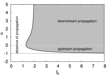
Figure 5: Regions where invasions are successful (gray) and unsuccessful (white) in the plane ($l_{f},u$). For $u>0$ we have downstream invasions. For $u<0$, upstream invasions are possible only for $-1<u<0$, see text for explanation. Data refer to the case $l_{u}=2$ and $\epsilon=1$.

The gray area in Fig. 5 displays the region in the plane ($l_{f},u$) where invasions are possible. Such a region was numerically determined by solving Eq. (14) and finding the values of $l_{f}$ and $u$ for which the propagation speed $u_{p}(u)=\min_{s}\{u_{p}(s;u)\}$ exists and is positive. For $u>0$ the curve, separating white and gray regions, coincides with that derived from Eq. (8) (shown in Fig. 3). For $u<0$, it approaches the asymptote $u=-1$ for large $l_{f}$. Indeed for very large favorable patches the system should recover the homogeneous habitat result $u_{p}=1+u$, so that invasions are impossible for $u<-1$ (Lutscher et al, 2006).

We now focus on the invasion speed $u_{p}$ for downstream invasions ($u>0$). The upstream case was considered in details by Lutscher et al (2006). Simulations (not shown) suggest that for $u\ll 1$ the invasion speed behaves linearly in $u$, i.e.

$$u_{p}(u)\approx u_{p}(0)+\alpha u\,,$$ (15)

both in region II and III. The above result holds also for small negative $u$. To determine $\alpha$ the first step is to expand $\mathcal{D}(u_{p},s;u)$ in powers of $u$. At the first order the expansion yields

$$\mathcal{D}(u_{p},s;u)=\mathcal{D}(u_{p},s;0)+f(s)u+O(u^{2})=0\,,$$ (16)

with $f(s)=L\sinh(Ls)$. For small $u$ the minimum of (16) is realized at $u_{p}(u)=u_{p}(0)+\delta u_{p}$ and $s(u)=s(0)+\delta s$, with $\delta u_{p},\delta s\sim O(u)$. Expanding now Eq. (16) in $\delta u_{p}$ and $\delta s$, one gets

$$\delta u_{p}=-\left[\frac{f(s(0))}{\left.\partial_{u_{p}}\mathcal{D}(u_{p},s;0)\right|_{u_{p}(0),s(0)}}\right]\,u=\alpha u\,.$$ (17)

From the numerical values of $u_{p}(0)$ and $s(0)$, we computed the value of $\alpha$ obtaining a perfect agreement with simulations.

We now consider the behavior of the invasion speed for large advection velocities. When $l_{f}$ is chosen in region II the invasion is halted for $u>u_{c}$. In region III, the population can invade the habitat for any $u$ and the invasion speed approaches another linear behavior for $u\gg 1$. In Fig. 6, we contrast two cases: when $l_{f}=\epsilon l_{u}$ and $l_{f}>\epsilon l_{u}$, inside region III.

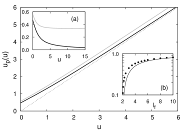
Figure 6: Invasion speed $u_{p}$ vs $u$ for $l_{f}=2$ (black curve) and $l_{f}=2.5$ (gray curve), together with the linear behavior $u_{p}=u$ (dotted line). Inset (a): $u_{p}-u$ vs $u$ for $l_{f}=2$ (black curve) and $l_{f}=2.5$ (gray curve). Inset (b): $u_{p}-u$ vs $l_{f}$ (symbols) compared with the asymptotic prediction (18), approximated in the simulation using $u=100$. Data have been obtained with $l_{u}=2$ and $\epsilon=1$.

As discussed in Sect. 4.1.2, when $l_{f}=\epsilon l_{u}$, the average biomass vanishes ($B(u)\to 0$) for $u\to u_{c}=\infty$. It is thus reasonable to expect that the contribution to the invasion speed comes only from advection. Therefore, asymptotically we expect $u_{p}\to u$ as shown in Fig. 6, though the convergence of $u_{p}-u$ to zero can be rather slow (Fig. 6a). Conversely, inside region III, $u_{p}-u$ reaches a finite value for $u\to\infty$ (Fig. 6a). As heuristically derived in D, for $u\gg 1$ one expects

$$u_{p}(u)-u={\Delta}/{l_{f}}\,,$$ (18)

where $\Delta=l_{f}-\epsilon l_{u}$. Strictly speaking, the above result holds in the limit of $u\to\infty$ and $l_{f}\to\infty$ but, as shown in Fig. 6(b), it is in fairly good agreement with the numerical results also for finite values of $l_{f}$.

To summarize, in region III the invasion speed $u_{p}$ is well approximated by two different linear behaviors

$${}\left\{\begin{array}[]{ll}u_{p}(u)\simeq u_{p}(0)+\alpha u&\quad\mbox{for small }u\vspace{0.2truecm}\\ u_{p}(u)\simeq{\displaystyle\Delta}/{\displaystyle l_{f}}+u&\quad\mbox{for large }u\end{array}\right.$$ (19)

where $\alpha$ is given by Eq. (17).

4.2.1 Invasion speed in rapidly and slowly varying environments

We now study the invasion speed in two limiting cases for which some analytical results can be obtained, namely when the habitat is finely fragmented ($l_{u,f}\ll 1$) or subdivided in large patches ($l_{u,f}\gg 1$ with $\gamma=l_{f}/l_{u}$ fixed).

When $l_{f,u}\ll 1$, expanding Eq. (14) at the lowest order, one obtains the explicit expression

$$u_{p}(s;u)\approx\frac{s}{2}+\left(\frac{\Delta}{L}\right)\frac{1}{2s}+u\,,$$ (20)

Retaining higher order terms, it is possible to show that the dependence of $u_{p}$ on $u$ is linear up to the fourth order in $l_{f,u}$, where a term proportional to $u^{2}$ appears. Minimizing Eq. (20) yields

$$u_{p}(u)=\mathchoice{{\hbox{$\displaystyle\sqrt{{\Delta}/{L}\,}$}\lower 0.4pt\hbox{\vrule height=7.5pt,depth=-6.00003pt}}}{{\hbox{$\textstyle\sqrt{{\Delta}/{L}\,}$}\lower 0.4pt\hbox{\vrule height=7.5pt,depth=-6.00003pt}}}{{\hbox{$\scriptstyle\sqrt{{\Delta}/{L}\,}$}\lower 0.4pt\hbox{\vrule height=5.25pt,depth=-4.20003pt}}}{{\hbox{$\scriptscriptstyle\sqrt{{\Delta}/{L}\,}$}\lower 0.4pt\hbox{\vrule height=3.75pt,depth=-3.00002pt}}}+u\,,$$ (21)

as also obtained with homogenization techniques (Lutscher et al, 2006). Equation (21) shows that for finely fragmented habitats the intrinsic propagation speed is as in the homogeneous habitat once the growth rate is substituted with the average growth rate $\Delta/L$, as found by Shigesada et al (1986) for $u=0$. Moreover, Eq. (21) implies that for $l_{u,f}\to 0$, $\alpha$ in Eq. (15) is equal to unity. We finally observe that Eq. (21) holds only for $\Delta\geq 0$, that is in region III of Fig. 3. Indeed for $l_{u,f}\to 0$ region II shrinks to zero.

In the limit of very large patch sizes, $l_{f,u}\rightarrow\infty$, from Eq. (14) we obtain

$$q_{0}L=q_{u}l_{u}+q_{f}l_{f}\,,$$ (22)

where $q_{0}\!=\!u\!+\!s$, $q_{u}\!=\!\mathchoice{{\hbox{$\displaystyle\sqrt{u^{2}\!+\!\epsilon\!+\!2su_{p}\,}$}\lower 0.4pt\hbox{\vrule height=6.44444pt,depth=-5.15558pt}}}{{\hbox{$\textstyle\sqrt{u^{2}\!+\!\epsilon\!+\!2su_{p}\,}$}\lower 0.4pt\hbox{\vrule height=6.44444pt,depth=-5.15558pt}}}{{\hbox{$\scriptstyle\sqrt{u^{2}\!+\!\epsilon\!+\!2su_{p}\,}$}\lower 0.4pt\hbox{\vrule height=4.51111pt,depth=-3.6089pt}}}{{\hbox{$\scriptscriptstyle\sqrt{u^{2}\!+\!\epsilon\!+\!2su_{p}\,}$}\lower 0.4pt\hbox{\vrule height=3.44165pt,depth=-2.75334pt}}}$ and $q_{f}\!=\!\mathchoice{{\hbox{$\displaystyle\sqrt{u^{2}\!-\!1\!+\!2su_{p}\,}$}\lower 0.4pt\hbox{\vrule height=6.44444pt,depth=-5.15558pt}}}{{\hbox{$\textstyle\sqrt{u^{2}\!-\!1\!+\!2su_{p}\,}$}\lower 0.4pt\hbox{\vrule height=6.44444pt,depth=-5.15558pt}}}{{\hbox{$\scriptstyle\sqrt{u^{2}\!-\!1\!+\!2su_{p}\,}$}\lower 0.4pt\hbox{\vrule height=4.51111pt,depth=-3.6089pt}}}{{\hbox{$\scriptscriptstyle\sqrt{u^{2}\!-\!1\!+\!2su_{p}\,}$}\lower 0.4pt\hbox{\vrule height=3.44165pt,depth=-2.75334pt}}}$ (see C). It is interesting to compute the limit maintaining the ratio $\gamma=l_{f}/l_{u}$ constant so that Eq. (22) becomes $q_{0}(1+\gamma)=q_{u}+\gamma q_{f}$, which has the explicit form

$$(1\!+\!\!\gamma)(u\!+\!s)\!=\!\!\mathchoice{{\hbox{$\displaystyle\sqrt{u^{2}\!+\!\!\epsilon\!+\!2u_{p}s\,}$}\lower 0.4pt\hbox{\vrule height=6.44444pt,depth=-5.15558pt}}}{{\hbox{$\textstyle\sqrt{u^{2}\!+\!\!\epsilon\!+\!2u_{p}s\,}$}\lower 0.4pt\hbox{\vrule height=6.44444pt,depth=-5.15558pt}}}{{\hbox{$\scriptstyle\sqrt{u^{2}\!+\!\!\epsilon\!+\!2u_{p}s\,}$}\lower 0.4pt\hbox{\vrule height=4.51111pt,depth=-3.6089pt}}}{{\hbox{$\scriptscriptstyle\sqrt{u^{2}\!+\!\!\epsilon\!+\!2u_{p}s\,}$}\lower 0.4pt\hbox{\vrule height=3.44165pt,depth=-2.75334pt}}}\!+\!\!\gamma\mathchoice{{\hbox{$\displaystyle\sqrt{u^{2}\!\!-\!1\!+\!2u_{p}s\,}$}\lower 0.4pt\hbox{\vrule height=6.44444pt,depth=-5.15558pt}}}{{\hbox{$\textstyle\sqrt{u^{2}\!\!-\!1\!+\!2u_{p}s\,}$}\lower 0.4pt\hbox{\vrule height=6.44444pt,depth=-5.15558pt}}}{{\hbox{$\scriptstyle\sqrt{u^{2}\!\!-\!1\!+\!2u_{p}s\,}$}\lower 0.4pt\hbox{\vrule height=4.51111pt,depth=-3.6089pt}}}{{\hbox{$\scriptscriptstyle\sqrt{u^{2}\!\!-\!1\!+\!2u_{p}s\,}$}\lower 0.4pt\hbox{\vrule height=3.44165pt,depth=-2.75334pt}}}.$$ (23)

The above formula does not depend on $l_{u}$ and $l_{f}$ separately but only on their ratio $\gamma$, meaning that for $l_{u,f}\to\infty$ the propagation speed $u_{p}$ approaches a limit value that depends only on $\gamma$ and $\epsilon$. The limits $\gamma\gg 1$ and $\gamma\ll 1$ are quite trivial and consistent with intuition. In both cases, neglecting sub-leading terms, squaring both sides of (23) one finds $u_{p}(s)$. In the former limit, $l_{f}\gg l_{u}$ (negligible unfavorable patches), the homogeneous result $u_{p}(u)=1+u$ is retrieved. In the latter, $l_{u}\gg l_{f}$ (negligible favorable patches), the condition for the minimum of $u_{p}(s;u)$ is realized for imaginary values of $s$, meaning that invasions are not possible.

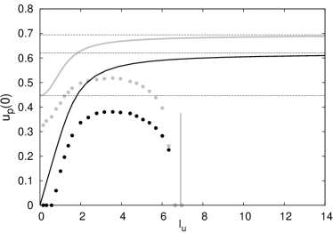
Figure 7: Invasion speed $u_{p}(0)$ vs $l_{u}$ with $\gamma=l_{f}/l_{u}$ fixed and $\epsilon=1$. Continuous lines correspond to the numerical solution of Eq. (14) for $\gamma=1$ (black) and $\gamma=1.5$ (gray). Dashed lines correspond to the limit values for rapidly and slowly varying environments, respectively. The former is zero for $\gamma=1$. Symbols show $u_{p}$ measured in numerical simulations with the Allee effect model (7) with $\theta_{c}=0.001$ (see Sect. 5). Black and gray symbols correspond to $\gamma=1$ and $1.5$, respectively. The vertical bar marks the critical unfavorable patch size (27) above which invasions are impossible.

In the special case $\gamma\!=\!1$ and $u\!=\!0$, Eq. (23) becomes $2s=\mathchoice{{\hbox{$\displaystyle\sqrt{2u_{p}s+\epsilon\,}$}\lower 0.4pt\hbox{\vrule height=6.44444pt,depth=-5.15558pt}}}{{\hbox{$\textstyle\sqrt{2u_{p}s+\epsilon\,}$}\lower 0.4pt\hbox{\vrule height=6.44444pt,depth=-5.15558pt}}}{{\hbox{$\scriptstyle\sqrt{2u_{p}s+\epsilon\,}$}\lower 0.4pt\hbox{\vrule height=4.51111pt,depth=-3.6089pt}}}{{\hbox{$\scriptscriptstyle\sqrt{2u_{p}s+\epsilon\,}$}\lower 0.4pt\hbox{\vrule height=3.22221pt,depth=-2.57779pt}}}+\mathchoice{{\hbox{$\displaystyle\sqrt{2u_{p}s-1\,}$}\lower 0.4pt\hbox{\vrule height=6.44444pt,depth=-5.15558pt}}}{{\hbox{$\textstyle\sqrt{2u_{p}s-1\,}$}\lower 0.4pt\hbox{\vrule height=6.44444pt,depth=-5.15558pt}}}{{\hbox{$\scriptstyle\sqrt{2u_{p}s-1\,}$}\lower 0.4pt\hbox{\vrule height=4.51111pt,depth=-3.6089pt}}}{{\hbox{$\scriptscriptstyle\sqrt{2u_{p}s-1\,}$}\lower 0.4pt\hbox{\vrule height=3.22221pt,depth=-2.57779pt}}}$, from which it is easy to derive the invasion speed:

$$u_{p}(0)=2\frac{1+\epsilon^{2}+(1-\epsilon)\mathchoice{{\hbox{$\displaystyle\sqrt{1+\epsilon+\epsilon^{2}\,}$}\lower 0.4pt\hbox{\vrule height=6.44444pt,depth=-5.15558pt}}}{{\hbox{$\textstyle\sqrt{1+\epsilon+\epsilon^{2}\,}$}\lower 0.4pt\hbox{\vrule height=6.44444pt,depth=-5.15558pt}}}{{\hbox{$\scriptstyle\sqrt{1+\epsilon+\epsilon^{2}\,}$}\lower 0.4pt\hbox{\vrule height=4.51111pt,depth=-3.6089pt}}}{{\hbox{$\scriptscriptstyle\sqrt{1+\epsilon+\epsilon^{2}\,}$}\lower 0.4pt\hbox{\vrule height=3.44165pt,depth=-2.75334pt}}}}{\left(1-\epsilon+2\mathchoice{{\hbox{$\displaystyle\sqrt{1+\epsilon+\epsilon^{2}\,}$}\lower 0.4pt\hbox{\vrule height=6.44444pt,depth=-5.15558pt}}}{{\hbox{$\textstyle\sqrt{1+\epsilon+\epsilon^{2}\,}$}\lower 0.4pt\hbox{\vrule height=6.44444pt,depth=-5.15558pt}}}{{\hbox{$\scriptstyle\sqrt{1+\epsilon+\epsilon^{2}\,}$}\lower 0.4pt\hbox{\vrule height=4.51111pt,depth=-3.6089pt}}}{{\hbox{$\scriptscriptstyle\sqrt{1+\epsilon+\epsilon^{2}\,}$}\lower 0.4pt\hbox{\vrule height=3.44165pt,depth=-2.75334pt}}}\,\right)^{3/2}}.$$ (24)

Notice that, once the proper correspondence between notations is made, the result (24) coincides with that obtained by Hamel et al (2010) using a different technique. Further specializing to the case of equal growth and death rates ($\epsilon=1$) Eq. (24) reduces to $u_{p}(0)=2^{1/2}3^{-3/4}$.

In the presence of advection with $u\ll 1$, the computation for $\gamma=1$ and $\epsilon=1$ can be easily extended obtaining $u_{p}(u)=2^{1/2}3^{-3/4}+(2/3)u$ that is Eq. (15) with $\alpha=2/3$. For $u\gg 1$, we were unable to obtain analytical results, but we expect the phenomenology discussed in Fig. 6 to apply.

In Fig. 7 we show the invasion speed $u_{p}$, obtained by numerically solving (14) for $u=0$, at varying $l_{u,f}$ with $\gamma=l_{f}/l_{u}=1$ and $1.5$. We also show the asymptotic values for $l_{u,f}\to 0$ and $l_{u,f}\to\infty$. In rapidly varying environments $u_{p}(0)=\mathchoice{{\hbox{$\displaystyle\sqrt{(\gamma-\epsilon)/(1+\gamma)\,}$}\lower 0.4pt\hbox{\vrule height=7.5pt,depth=-6.00003pt}}}{{\hbox{$\textstyle\sqrt{(\gamma-\epsilon)/(1+\gamma)\,}$}\lower 0.4pt\hbox{\vrule height=7.5pt,depth=-6.00003pt}}}{{\hbox{$\scriptstyle\sqrt{(\gamma-\epsilon)/(1+\gamma)\,}$}\lower 0.4pt\hbox{\vrule height=5.25pt,depth=-4.20003pt}}}{{\hbox{$\scriptscriptstyle\sqrt{(\gamma-\epsilon)/(1+\gamma)\,}$}\lower 0.4pt\hbox{\vrule height=3.75pt,depth=-3.00002pt}}}$ while in slowly varying ones $u_{p}(0)$ goes to the finite value (23) which for $\gamma=1$ is given by (24).

4.2.2 Efficiency of the invasion process as a function of the advection velocity

The invasion speed $u_{p}$ measures the velocity of population advancement. We now focus on the rate of increase of the population size (inset of Fig. 1a), which provides a measure of the efficiency of the invasion process. The suitable quantity to look at is the rate of increase of the total biomass

$$B_{r}(u)=\frac{\mathrm{d}}{\mathrm{d}t}\int_{0}^{\infty}\theta(x,t){\mathrm{d}}x\,,$$

which is the slope of the curve shown in the inset of Fig. 1a.

Figure 8: Rate of increase of the biomass $B_{r}(u)$ vs $u$ for $\epsilon=1$, $l_{u}=2$ and $l_{f}=1.5$ (boxes) and $l_{f}=1.8$ (circles) (see also Fig. 4).

Figure 8 shows that there is an optimal advection velocity which maximizes the rate $B_{r}(u)$. So that, in spite of the fact that larger advection velocities imply larger invasion speeds, the efficiency of the invasion process is maximized at a specific value $u^{\ast}$ of the advection velocity. This means that even though for $u>u^{\ast}$ the invasion speed increases, the number of invading individuals decreases, which implies a less effective invasion.

We now provide a heuristic argument to explain the origin of an optimal advection velocity. At stationarity, the population, advancing at constant speed $u_{p}(u)$, increases its size at a rate

$$B_{r}(u)=\,B(u)u_{p}(u)$$ (25)

where $B(u)$ is the average biomass (10). For $u\ll 1$, $B(u)$ is well described by Eq. (11), i.e. $B(u)$ decreases quadratically with $u$. On the other hand, as from Eq. (15), the invasion speed increases linearly with $u$. Using the above considerations and Eq. (25), we obtain that the increase in invasion speed will dominate at very small $u$ while the quadratic decrease of $B(u)$ will dominate at larger $u$, producing the bell shaped behavior observed in Fig. 8.

The above argument is based on a low order Taylor expansion which, in principle, could cease to be valid for values of $u$ at which the maximum of $B_{r}(u)$ is attained. We numerically found that the behavior reported in Fig. 8 is general and that, typically, the maximum of $B_{r}(u)$ is realized for values of $u$ for which the Taylor expansion is still a valid approximation.

4.3 Discussions

Shigesada et al (1986) have shown that even when the average growth rate is negative (i.e. $\Delta=l_{f}-\epsilon l_{u}<0$) there exists a critical size of the favorable patches above which a population can invade new territories. We have shown that the main effect of advection is to increase the critical size $l_{f}^{*}$ for the invasion to be possible. In particular, there always exists a critical advection velocity $u_{c}$ above which no invasion is possible, unless the average growth rate is positive.

As for the invasion speed, we recover the results obtained for $u=0$ by Shigesada et al (1986), and for $u\neq 0$ by Lutscher et al (2006), who focused on upstream propagation (i.e. in our setting $u<0$). However, here, we mainly focused on the downstream invasion speed, i.e. when the advection velocity favors the invasion ($u>0$). Our analysis shows that, provided $u<u_{c}$, advection always increases the invasion speed. In particular, both for small and large advection velocities $u$ the invasion speed is linear in $u$ but with different prefactors (see Eq. (19)). In some interesting environmental limits, moreover, we analytically computed the invasion speed. Our results agree with those found with different techniques by Hamel et al (2010), and are interesting in view of the ensuing discussion on Allee effects.

Our results on the dependence of the population size (the biomass) on advection extend similar ones derived by Dahmen et al (2000) in the limit of large unfavorable patches. Although the invasion speed is enhanced by advection, the biomass decreases at increasing the advection velocity. As a consequence, a faster invasion speed does not necessarily imply a more efficient invasion process. Indeed, the suitable quantity to judge about the effectiveness of the invasion process is the rate of increase of the biomass. We found the remarkable new result of an optimal advection velocity maximizing such rate and, hence, the efficiency of the invasion process. This maximum originates from the opposite role of advection on the invasion speed $u_{p}$ and on the biomass $B(u)$: the former increases linearly with $u$ while the latter decreases quadratically with $u$. The balance between these two behaviors leads to a maximum in the invasion efficiency.

5 Results for the Allee effect growth model

Some features of the logistic model seem quite unreasonable from an ecological point of view. For instance, as shown in Fig. 7, the invasion speed approaches an asymptotic value when the sizes of the patches are enlarged holding fixed their ratio, regardless of the size of hostile regions (i.e. even for $l_{u}\to\infty$). Intuition would suggest that extremely large unfavorable regions should slowdown, and eventually suppress, invasions, as observed, e.g., in soil organisms (Bailey et al, 2000). A slowdown of the invasion process should be expected, indeed, anytime there is a positive correlation between population density and per capita growth rate, i.e. in the presence of Allee effects (Allee, 1938; Dennis, 1989). In general, one speaks of Allee effect when for small densities the growth rate is negative — strong Allee effect — or positive, but smaller than for larger density — weak Allee effect (Wang and Kot, 2001). Relevant works and their relations with our problem are discussed in the next section (in particular, see Table 1).

We consider the Allee effect threshold model (7), that we recall here

$$g_{f}(\theta)=\max\{(\theta-\theta_{c})(1-\theta),0\}\,.$$ (26)

This model corresponds to a situation in between the strong and weak Allee effect and is convenient because it reduces to the logistic model (6) for $\theta_{c}\!=\!0$, easing the comparison. At the end of this section we will briefly discuss different Allee effect models.

Studying the problem without advection allows us to identify the main consequence of the Allee effect, namely the existence of a critical unfavorable patch size $l^{*}_{u}$ above which invasion is impossible for any size of the favorable region and the population can persist localized as shown in Fig. 2. At stationarity, in the bulk of the traveling front we have that, if $\theta_{M}$ is the value at the beginning of an unfavorable patch, then at the end of the unfavorable region the density will reach the value $\theta_{m}=\theta_{M}\exp\left(-\mathchoice{{\hbox{$\displaystyle\sqrt{\epsilon\,}$}\lower 0.4pt\hbox{\vrule height=4.30554pt,depth=-3.44446pt}}}{{\hbox{$\textstyle\sqrt{\epsilon\,}$}\lower 0.4pt\hbox{\vrule height=4.30554pt,depth=-3.44446pt}}}{{\hbox{$\scriptstyle\sqrt{\epsilon\,}$}\lower 0.4pt\hbox{\vrule height=3.01389pt,depth=-2.41113pt}}}{{\hbox{$\scriptscriptstyle\sqrt{\epsilon\,}$}\lower 0.4pt\hbox{\vrule height=2.15277pt,depth=-1.72223pt}}}l_{u}\right)$. Given the growth term (26), for the population to propagate we must require that $\theta_{m}\geq\theta_{c}$ (see also Dewhirst and Lutscher (2009) for a similar argument applied to an integro-difference model), which implies the inequality

$$l_{u}\leq l^{*}_{u}=\frac{1}{\mathchoice{{\hbox{$\displaystyle\sqrt{\epsilon\,}$}\lower 0.4pt\hbox{\vrule height=4.30554pt,depth=-3.44446pt}}}{{\hbox{$\textstyle\sqrt{\epsilon\,}$}\lower 0.4pt\hbox{\vrule height=4.30554pt,depth=-3.44446pt}}}{{\hbox{$\scriptstyle\sqrt{\epsilon\,}$}\lower 0.4pt\hbox{\vrule height=3.01389pt,depth=-2.41113pt}}}{{\hbox{$\scriptscriptstyle\sqrt{\epsilon\,}$}\lower 0.4pt\hbox{\vrule height=2.15277pt,depth=-1.72223pt}}}}\log\left(\frac{\theta_{M}}{\theta_{c}}\right)$$ (27)

for the unfavorable patch size. In general, $\theta_{M}$ cannot be estimated analytically; however, setting $\theta_{M}\!=\!1$ gives a reasonable upper bound.

The existence of $l^{*}_{u}$ is evident from Fig. 7 where symbols denote the results of numerical simulations obtained with the growth model (26), holding constant $\gamma=l_{f}/l_{u}$ and increasing the patch sizes. For small sizes the qualitative behavior of the model (26) is similar to that of the logistic model: $u_{p}$ increases with $L$. A dramatic difference appears at large sizes: for the logistic model the invasion speed reaches an asymptotic value, while for the Allee effect one it decreases and, eventually, the invasion process is halted when $l_{u}\approx l_{u}^{*}$, regardless the size of the favorable patch.

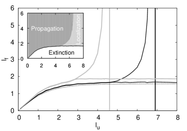
Figure 9: Regions of the plane $(l_{u},l_{f})$ characterized by localization, propagation and extinction of the population with the Allee effect model (26) with $u=0$, $\epsilon=1$, $\theta_{c}=0.001$ (black) and $\theta_{c}=0.01$ (gray). For each value of $\theta_{c}$, two curves separate the three different possibilities as shown in the inset with shaded areas for the case $\theta_{c}=0.001$. The vertical lines in the main figure show $l_{u}^{*}$ obtained from (27) with $\theta_{M}=1$. The dotted curve displays the dependence of $l_{f}^{*}$ for the logistic model (6).

In Figure 9, we show the behavior of the system without advection in the plane $(l_{u},l_{f})$, for two values of $\theta_{c}$. As already discussed, for the logistic growth model there exists a critical favorable patch size $l_{f}^{*}$ above which the population can survive and invade new territories. The critical value $l_{f}^{*}$ remains finite for $l_{u}\to\infty$ as found by Ludwig et al (1979); Shigesada et al (1986) and also in this paper. With the Allee effect growth model (26) the phenomenology is different and more interesting. When the size of the unfavorable patches is small (i.e. $l_{u}\ll 1$) the system essentially behaves as the logistic model: the unfavorable patch is so small that typically the decrease in density will not cause the population to fall below $\theta_{c}$. From a quantitative point of view, $l_{f}^{*}$ is slightly larger than the logistic value (the effect being more pronounced for larger $\theta_{c}$), though this cannot be fully appreciated from Fig. 9 due to the scale. The main qualitative change with respect to the logistic case manifests when the size of the unfavorable patches approaches the value $l_{u}^{*}$ given in Eq. (27). For unfavorable patches at least this large, propagation becomes impossible for any size of the favorable patches, even though the population does not necessarily go extinct. Indeed, as highlighted in the inset of Fig. 9, a new region in the plane $(l_{u},l_{f})$ appears, where the population can persist locally but cannot propagate (see Fig. 2): it localizes in a single favorable patch (if initially it was in that patch). For this localization regime to exist it is necessary that $l_{f}$ is wide enough to sustain the population, as theoretically derived in the homogeneous case by Lewis and Kareiva (1993) and found in field data by Vercken et al (2011).

Therefore, without advection but with the Allee effect growth term (26), we have that the population goes extinct if $l_{f}<l_{f}^{*}$, propagates if $l_{f}>l_{f}^{*}$ but $l_{u}<l_{u}^{*}$, and localizes in a single favorable patch when this is large enough to sustain the population ($l_{f}>l_{f}^{*}$) but the unfavorable patch is too large to allow the propagation, i.e. $l_{u}\geq l_{u}^{*}$.

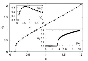
Figure 10: Invasion speed $u_{p}$ vs $u$ for the Allee effect model (26) with $\theta_{c}=0.001$, $\epsilon=1$ and $l_{u}\!=\!l_{f}\!=\!8$, i.e. within the localization region of Fig. 9. Gray symbols correspond to values of $u$ for which the population remains localized, while black ones to values for which it propagates. Inset (a): rate of increase of the biomass $B_{r}$ vs $u$ obtained using the same parameters of the main figure. Inset (b): invasion speed vs $l_{f}$ for $u=0.2$ and $l_{u}=8$. At increasing $l_{f}$ the population passes from extinction (empty symbols) to localization (gray symbols) and finally to propagation (black symbols). The last transition is possible only thanks to advection.

We now discuss the effects of advection. For small unfavorable patch sizes, $l_{u}\ll 1$, since the model with Allee effect behaves quite similarly to the logistic model, also the effect of advection on the dynamics is very similar between the two models. A critical advection velocity $u_{c}$ exists, above which the population goes extinct. However, for larger unfavorable patches, while in the absence of advection propagation is inhibited and the population remains localized (light gray region in the inset of Fig. 9), sustained advection induces the remarkable qualitative changes observed in Fig. 2. In Fig. 10 we show a numerical measurement of the invasion speed $u_{p}$ as a function of $u$ for a habitat with unfavorable and favorable patch sizes, $l_{u}$ and $l_{f}$ respectively, chosen in the localization region of the system without advection. As it can be seen, while the population remains localized at small advection velocities, it suddenly becomes able to propagate invading the whole environment when the velocity of the medium becomes large enough. An intuitive explanation for such a behavior is that, thanks to advection, the population can now travel through the unfavorable patch more rapidly, finally reaching the next favorable patch with a density above the threshold $\theta_{c}$, i.e., advection enhances the value $l_{u}^{*}$ above which no propagation is possible. In fact, at stationarity, in the unfavorable region it is easy to see that the density behaves as $\theta(x)=\theta_{M}\exp[(u-\mathchoice{{\hbox{$\displaystyle\sqrt{\epsilon+u^{2}\,}$}\lower 0.4pt\hbox{\vrule height=6.10999pt,depth=-4.88802pt}}}{{\hbox{$\textstyle\sqrt{\epsilon+u^{2}\,}$}\lower 0.4pt\hbox{\vrule height=6.10999pt,depth=-4.88802pt}}}{{\hbox{$\scriptstyle\sqrt{\epsilon+u^{2}\,}$}\lower 0.4pt\hbox{\vrule height=4.30276pt,depth=-3.44223pt}}}{{\hbox{$\scriptscriptstyle\sqrt{\epsilon+u^{2}\,}$}\lower 0.4pt\hbox{\vrule height=3.44165pt,depth=-2.75334pt}}})x]$. Therefore, the same argument which lead to Eq. (27) now yields

$$l_{u}^{*}(u)=\frac{1}{\mathchoice{{\hbox{$\displaystyle\sqrt{\epsilon+u^{2}\,}$}\lower 0.4pt\hbox{\vrule height=6.10999pt,depth=-4.88802pt}}}{{\hbox{$\textstyle\sqrt{\epsilon+u^{2}\,}$}\lower 0.4pt\hbox{\vrule height=6.10999pt,depth=-4.88802pt}}}{{\hbox{$\scriptstyle\sqrt{\epsilon+u^{2}\,}$}\lower 0.4pt\hbox{\vrule height=4.30276pt,depth=-3.44223pt}}}{{\hbox{$\scriptscriptstyle\sqrt{\epsilon+u^{2}\,}$}\lower 0.4pt\hbox{\vrule height=3.44165pt,depth=-2.75334pt}}}-u}\log\left(\frac{\theta_{M}}{\theta_{c}}\right)\,.$$

The above formula predicts that $l_{u}^{*}(u)$ grows with $u$, so that even if in a medium at rest the population is localized, i.e. $l_{u}>l_{u}^{*}(0)$, in advective media there will be a value of the advection velocity such that $l_{u}\leq l_{u}^{*}(u)$, allowing the population to propagate, as shown in Fig. 10. Once invasion is permitted by advection, the propagation speed and the rate of increase of biomass behave similarly to the same quantities in the logistic model (compare Fig. 10 main figure with Fig. 6 main figure, and Fig. 10a with Fig. 8).

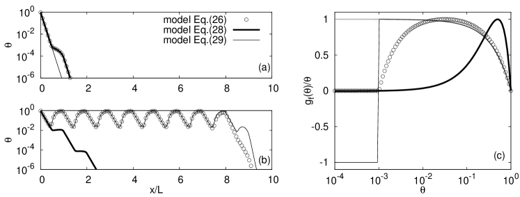
Figure 11: Advection-induced invasions for different Allee effect models with $\theta_{c}\!=\!0.001$, $l_{u}\!=\!8$, $l_{f}\!=\!7$ and $\epsilon\!=\!1$. (a) With $u\!=\!0$ the population evolving with the Allee effect models as labeled is unable to invade. (b) With $u\!=\!0.5$ invasion is possible but for the cubic model (28). As for model (29) we used $b\!=-1$. (c) Comparison of the per capita growth rates $g_{f}(\theta)/\theta$ in the three considered models together with the logistic case $g_{f}(\theta)/\theta\!=\!1\!-\!\theta$ (gray line). Notice that for comparison purposes all models have been normalized in a such a way that $\max_{\theta}\{g_{f}(\theta)/\theta\}=1$.

The results shown in the inset (b) of Fig. 10 further illustrate the importance of advection in such model. There, we show the measured propagation velocity $u_{p}$ as a function of $l_{f}$, for constant advection $u$ and keeping $l_{u}>l_{u}^{*}(0)$ fixed, so that in the absence of advection the population would be localized even if $l_{f}>l_{f}^{*}$. As one can see two transitions are observed: from extinction to localized, mainly due to the increase of $l_{f}$; from localized to propagating, which is possible only thanks to advection. It is interesting here to note that something similar happens if we consider a spatially dependent diffusion coefficient, as done by Shigesada et al (1986) for the logistic growth model. In particular, without advection ($u=0$) and denoting with $\delta=D_{u}/D_{f}$ the ratio between diffusivities in the unfavorable and favorable patches, Eq. (27) modifies in $l_{u}^{*}\approx\mathchoice{{\hbox{$\displaystyle\sqrt{\delta/\epsilon\,}$}\lower 0.4pt\hbox{\vrule height=7.5pt,depth=-6.00003pt}}}{{\hbox{$\textstyle\sqrt{\delta/\epsilon\,}$}\lower 0.4pt\hbox{\vrule height=7.5pt,depth=-6.00003pt}}}{{\hbox{$\scriptstyle\sqrt{\delta/\epsilon\,}$}\lower 0.4pt\hbox{\vrule height=5.25pt,depth=-4.20003pt}}}{{\hbox{$\scriptscriptstyle\sqrt{\delta/\epsilon\,}$}\lower 0.4pt\hbox{\vrule height=3.75pt,depth=-3.00002pt}}}\ln(\theta_{M}/\theta_{c})$. This result tells us that a larger diffusivity in the unfavorable regions ($\delta>1$) allows the population to propagate also with larger unfavorable patch sizes. Therefore, if we fix the size of the unfavorable patch, either increasing the diffusivity or the advection, the residence time in the unfavorable patch decreases leading to a smaller depletion in population density.

Through this section we limited the numerical analysis to the Allee effect model (26) which is intermediate between the case of weak and strong Allee effect. It is thus worth to test the robustness of the above findings by considering different Allee effect models. In Figure 11 we show the evolution of invasions obtained with three different models of the Allee effect, either in the absence (Fig. 11a) or in the presence (Fig. 11b) of advection when $l_{u}>l_{u}^{*}$. In particular, we compare model (26) with two models of Allee effect, namely the standard cubic term used to model strong Allee effects (Lewis and Kareiva, 1993; Petrovskii and Li, 2003; Almeida et al, 2006)

$$g_{f}(\theta)=\theta(1-\theta)(\theta-\theta_{c})\,,$$ (28)

and a slight modification of the model introduced by Wang and Kot (2001)

$$g_{f}(\theta)=\left\{\begin{array}[]{ll}b\theta&\quad\;0\leq\theta\leq\theta_{c}\\ \theta(1-\theta)&\quad\;\theta_{c}<\theta\leq 1\end{array}\right.\,,$$ (29)

The latter can model either strong ($b<0$) or weak (if $0<b<1$ and $1-\theta_{c}>b$) Allee effect. The marginal case $b=0$, for small values of $\theta_{c}$, is practically indistinguishable from the Allee effect model (26). Figure 11a shows that with $u=0$ invasions are unsuccessful in all the considered models. For model (29) we only show the case $b=-1$. However, the result (not shown) holds also for positive (not too large) values of $b$, meaning that also with weak Allee effects the population can be localized. Advection (Fig. 11b) is able to activate the invasion process in all cases but for the cubic model (28). The origin of such a difference is readily understandable from Fig. 11c where we show the density-dependent per capita growth rate $g_{f}(\theta)/\theta$ in the above models compared with the logistic case (the gray line). As one can see, the growth rate for the cubic model, although positive, remains very small for a large interval above the threshold value $\theta_{c}$. As a consequence, even if the population reaches the favorable region with $\theta>\theta_{c}$, it cannot propagate. In the other cases the growth rate is large enough to allow the population to grow and propagate.

Concluding, the phenomenology of the advection-induced invasion is rather general in the presence of (either weak or strong) Allee effect, but critically depends on the growth rate realized close to the threshold value $\theta_{c}$. In perspective, it would be interesting to investigate what habitat/advection conditions ensure successful invasions for different kinds of Allee effects.

	habitat	dispersal	references
invasion	homogeneous	diffusion	Lewis and
		(short range)	van den Driessche (1993),
			Hastings (1996),
			Wang and Kot (2001)
invasion,	homogeneous	diffusion+advection	Lewis and Kareiva (1993),
persistence,		(short+long range)	Petrovskii and Li (2003),
localization			Almeida et al. (2006)
persistence	heterogeneous	diffusion	Shi and Shivaji (2006)
		(short range)
invasion,	heterogeneous	diffusion+advection	This work
localization,		(short + long range)
persistence
invasion,	heterogeneous	dispersal kernel	Dewhirst and
localization,		(long range)	Lutscher (2009),
persistence		(special case: diffusion)	Pachepsky and
			Levine (2011)

Table 1: Models with Allee effects related to the present work. The models in the upper part of the table are advection-reaction-diffusion models; those in the lower part of the table are integro-difference models. Further details about models of Allee effects in invasion dynamics can be found in tables $3.5$ and $3.6$ in Courchamp et al (2008). Our work aims at investigating conditions for persistence and invasion in heterogeneous environments with advection.

5.1 Discussions

To put in perspective our results on the Allee effect model it is useful first to briefly recall some known results from the literature. The study of Allee effects has received considerable interest in the past, with growing modeling efforts in recent years, when its importance for invasions and conservation issues have started to be well recognized (Taylor and Hastings, 2005; Courchamp et al, 2008; Tobin et al, 2011). For convenience of the reader, we summarize relevant works related to our problem in Table 1.

In the case of homogeneous environments and without advection, most studies have shown that the success of an invasion depends not only on the initial density, but also on the size of the initially occupied area (Lewis and Kareiva, 1993; Lewis and van den Driessche, 1993; Kot et al, 1996; Wang and Kot, 2001). Asymptotic rates of spread are typically reduced (see, e.g. Lewis and Kareiva, 1993), mostly because of the interplay between dispersal mechanisms and the reduced reproductive power at low densities. In discrete-space models (e.g., in Keitt et al, 2001) the interesting phenomenon of population localization (also called range pinning) occurs. The presence of advection can lead to nontrivial results when combined with density-dependent migration (Petrovskii and Li, 2003; Almeida et al, 2006).

In the case of heterogeneous habitats, with few exceptions (see, e.g., Shi and Shivaji (2006) who extended the critical patch size problem to the case of weak Allee effects), most works focused on integro-difference models (Dewhirst and Lutscher, 2009), sometimes accounting also for the effect of discreteness of the population (Pachepsky and Levine, 2011). These studies agree on the fact that the presence of Allee effects combined with habitat fragmentation generally penalizes the success of invasions or, at least, slows them down. In particular, crucial for the success of the invasion process is the size of bad patches (Dewhirst and Lutscher, 2009) with respect to the dispersal range. Moreover, the results of these models depend also on the choice of the dispersal kernel, which is typically poorly known (Hastings et al, 2005).

Our results show that logistic and Allee effect models qualitatively display the same features both in the presence and in the absence of advection when the unfavorable patches are not too large, including the nontrivial existence of an optimal advection velocity maximizing the invasion efficiency. However, in the Allee effect case, unlike the logistic model, if the unfavorable patches become too large invasions can be halted. When the Allee effect is included, in fact, if both $l_{u}$ and $l_{f}$ are large, the population can persist locally, but is unable to invade other patches, since it cannot cross unfavorable regions without being too severely damped. This means that while in the logistic case the thresholds for persistence and for invasions coincide, these are in general different when Allee effects are present. The same observation was made in the context of integro-difference models (Dewhirst and Lutscher, 2009), and it is substantiated also by field observations (Bailey et al (2000), see also Hastings et al (2005) and references therein).

Advection, however, can alter this picture: if its intensity exceeds a threshold value, the invasion process can be activated, provided that a large enough growth rate is realized at the population density when entering the favorable patches. This peculiar effect of advection, which as far as we know was not previously put into light, has obvious ecological implications for invasive species management strategies. For instance, the idea to induce Allee effects to control the invasion of alien species, which can be implemented in several ways (Tobin et al, 2011), should be pursued with extreme care in the presence of advection.

In summary, our results on persistence and invasion in the presence of Allee effects extend previous works done in the framework of reaction-diffusion models (with homogeneous habitat) and positively correlate also with the results of integro-difference models, emphasizing the subtle role of advection which was missed in that kind of models.

6 Conclusions

In this paper we focused on the role of advection on invasions in heterogeneous environments characterized by favorable and unfavorable patches.

On the one hand, we have shown that in the presence of habitat heterogeneity sufficiently intense advection can halt the invasion process. Moreover, we argued that the efficiency of the invasive process is properly quantified in terms of the rate of increase of the invading population. In particular, we found that the latter is maximal at intermediate values of the advection velocity.

On the other hand we have shown that in the presence of Allee effects, advection may be beneficial to the invasion process turning a persistent but non invading population into an invading one.

An important aspect in evaluating biological invasions, which has not been considered in our work, is related to the discrete nature of a population, which is made of individuals (Durrett and Levin, 1994; Okubo and Levin, 2001). We expect that considering also discrete effects may add further nontrivial effects due to demographic stochasticity, in particular close to the transition between successful and unsuccessful invasions. Works in these direction have started to appear (Snyder, 2003; Pachepsky and Levine, 2011). It would be interesting to study the effect of advection also in the presence of demographic stochasticity.

7 Acknowledgments

We thank A. Vulpiani, who contributed to the initial stage of this work, for fruitful discussions and interactions. MC acknowledges support from MIUR PRIN-2009PYYZM5 “Fluttuazioni: dai sistemi macroscopici alle nanoscale”.

Appendix A Conditions for persistence in a periodic system

Due to the habitat periodicity, and with the periodic BC, we can limit the analysis to the unit cell $[0:L)$. Denoting with $\vartheta$ a perturbation around the solution $\theta=0$, we have that $\vartheta$ is ruled by the linearized version of Eq. (5)

$$\partial_{t}\vartheta+2u\partial_{x}\vartheta=\partial^{2}_{x}\vartheta+\epsilon(x)\vartheta\,,$$ (30)

where $\epsilon(x)=-\epsilon$ in the unfavorable patches and $\epsilon(x)=1$ in the favorable ones. In the linear analysis framework, at leading order, one expects that $\vartheta=e^{\Lambda t}\psi(x)$ so that population extinction is a stable solution if $\Lambda<0$ and an unstable one if $\Lambda>0$. When unstable, the asymptotic solution will be a stationary and spatially periodic solution $\psi(x)$ as in Fig. 1a, otherwise if $\Lambda<0$ it decays exponentially as $\vartheta(x,t)=\psi(x)e^{-|\Lambda|t}$ (see inset of Fig. 1c). Plugging $\vartheta=e^{\Lambda t}\psi(x)$ into (30) we obtain the characteristic equation for the stationary state

$$\partial^{2}_{x}\psi-2u\partial_{x}\psi+(\epsilon(x)-\Lambda)\psi=0\,,$$ (31)

whose general solution is given by

$$\begin{array}[]{ll}\psi_{u}(x)=A^{u}_{1}e^{x\lambda^{(u)}_{1}}+A^{u}_{2}e^{x\lambda^{(u)}_{2}}&\;0\leq x<l_{u}\\ \psi_{f}(x)=A^{f}_{1}e^{x\lambda^{(f)}_{1}}+A^{f}_{2}e^{x\lambda^{(f)}_{2}}&\;l_{u}\leq x<L\,,\end{array}$$ (32)

where

$$\begin{array}[]{l}\lambda^{(u)}_{1,2}=u\pm\phantom{i}\mathchoice{{\hbox{$\displaystyle\sqrt{\epsilon+\Lambda+u^{2}\,}$}\lower 0.4pt\hbox{\vrule height=6.83331pt,depth=-5.46667pt}}}{{\hbox{$\textstyle\sqrt{\epsilon+\Lambda+u^{2}\,}$}\lower 0.4pt\hbox{\vrule height=6.83331pt,depth=-5.46667pt}}}{{\hbox{$\scriptstyle\sqrt{\epsilon+\Lambda+u^{2}\,}$}\lower 0.4pt\hbox{\vrule height=4.78333pt,depth=-3.82668pt}}}{{\hbox{$\scriptscriptstyle\sqrt{\epsilon+\Lambda+u^{2}\,}$}\lower 0.4pt\hbox{\vrule height=3.44165pt,depth=-2.75334pt}}}=u\pm b_{u}(\Lambda)\\ \lambda^{(f)}_{1,2}=u\pm i\mathchoice{{\hbox{$\displaystyle\sqrt{1-\Lambda-u^{2}\,}$}\lower 0.4pt\hbox{\vrule height=6.83331pt,depth=-5.46667pt}}}{{\hbox{$\textstyle\sqrt{1-\Lambda-u^{2}\,}$}\lower 0.4pt\hbox{\vrule height=6.83331pt,depth=-5.46667pt}}}{{\hbox{$\scriptstyle\sqrt{1-\Lambda-u^{2}\,}$}\lower 0.4pt\hbox{\vrule height=4.78333pt,depth=-3.82668pt}}}{{\hbox{$\scriptscriptstyle\sqrt{1-\Lambda-u^{2}\,}$}\lower 0.4pt\hbox{\vrule height=3.44165pt,depth=-2.75334pt}}}=u\pm ib_{f}(\Lambda)\end{array}$$ (33)

are the eigenvalues associated to Eq. (31). For a solution to exist it is sufficient to impose the continuity of densities $\psi_{u,f}(x)$ and fluxes $J_{u,f}(x)=[2u-\partial_{x}]\psi_{u,f}(x)$ at the boundaries between favorable and unfavorable regions. Notice that the conditions on fluxes are required when using space-dependent diffusion coefficient, as, for example, in Shigesada et al (1986) and Lutscher et al (2006). For constant diffusion coefficient, as here, it is enough to impose the continuity of derivatives of $\psi$.

Using Eq. (32) and imposing the aforementioned continuity conditions we obtain a linear system for the four constants $A^{u,f}_{1,2}$. Requiring that this linear system has a nontrivial solution we obtain

$$\cosh(uL)-\cos(b_{f}(\Lambda)l_{f})\cosh(b_{u}(\Lambda)l_{u})$$

$$=\frac{b_{u}^{2}(\Lambda)-b_{f}^{2}(\Lambda)}{2b_{u}(\Lambda)b_{f}(\Lambda)}\sin(b_{f}(\Lambda)l_{f})\sinh(b_{u}(\Lambda)l_{u})\,.$$ (34)

The largest value of $\Lambda$ solving the above equation determines the stability properties of the solution $\theta=0$. In particular, fixing the values of $l_{u}$, $\epsilon$ and $u$, it is possible to show that $\Lambda\geq 0$ whenever $l_{f}\geq l_{f}^{*}$, where $l_{f}^{*}$ solves Eq. (34) with $\Lambda=0$ (Shigesada et al, 1986; Nagylaki, 1975), i.e. Eq. (8). For $l_{f}<l_{f}^{*}$ the population always goes extinct. An equivalent critical value exists for the advection velocity, see main text. Let us notice that with $u=0$, the above condition reduces to that found by Shigesada et al (1986), i.e. $\mathchoice{{\hbox{$\displaystyle\sqrt{\epsilon\,}$}\lower 0.4pt\hbox{\vrule height=4.30554pt,depth=-3.44446pt}}}{{\hbox{$\textstyle\sqrt{\epsilon\,}$}\lower 0.4pt\hbox{\vrule height=4.30554pt,depth=-3.44446pt}}}{{\hbox{$\scriptstyle\sqrt{\epsilon\,}$}\lower 0.4pt\hbox{\vrule height=3.01389pt,depth=-2.41113pt}}}{{\hbox{$\scriptscriptstyle\sqrt{\epsilon\,}$}\lower 0.4pt\hbox{\vrule height=2.15277pt,depth=-1.72223pt}}}\tanh\left(\mathchoice{{\hbox{$\displaystyle\sqrt{\epsilon\,}$}\lower 0.4pt\hbox{\vrule height=4.30554pt,depth=-3.44446pt}}}{{\hbox{$\textstyle\sqrt{\epsilon\,}$}\lower 0.4pt\hbox{\vrule height=4.30554pt,depth=-3.44446pt}}}{{\hbox{$\scriptstyle\sqrt{\epsilon\,}$}\lower 0.4pt\hbox{\vrule height=3.01389pt,depth=-2.41113pt}}}{{\hbox{$\scriptscriptstyle\sqrt{\epsilon\,}$}\lower 0.4pt\hbox{\vrule height=2.15277pt,depth=-1.72223pt}}}{l_{u}}/{2}\right)=\tan\left({l_{f}}/{2}\right)\,$. For $l_{u}\ll 1$, the above equation tells us that $l_{f}^{*}\approx\epsilon l_{u}$. Notice that the average growth rate is given by $\left(l_{f}-\epsilon l_{u}\right)/L$ and that for $l_{f}>\epsilon l_{u}$ survival of the population is guaranteed by the fact that the average growth rate is positive. As the size of the unfavorable patches grows the critical (favorable) patch size approaches the limit value $l_{f}^{*}=2\arctan\mathchoice{{\hbox{$\displaystyle\sqrt{\epsilon\,}$}\lower 0.4pt\hbox{\vrule height=4.30554pt,depth=-3.44446pt}}}{{\hbox{$\textstyle\sqrt{\epsilon\,}$}\lower 0.4pt\hbox{\vrule height=4.30554pt,depth=-3.44446pt}}}{{\hbox{$\scriptstyle\sqrt{\epsilon\,}$}\lower 0.4pt\hbox{\vrule height=3.01389pt,depth=-2.41113pt}}}{{\hbox{$\scriptscriptstyle\sqrt{\epsilon\,}$}\lower 0.4pt\hbox{\vrule height=2.15277pt,depth=-1.72223pt}}}$ corresponding to the result of Ludwig et al (1979). The case $\epsilon\to\infty$, i.e. infinite mortality, corresponds to the KISS critical patch size $l_{f}^{*}=\pi$ (Skellam, 1951; Kierstead and Slobodkin, 1953).

Appendix B Derivation of the asymptotic expression for biomass.

At stationarity, for $u\gg 1$ we can disregard the diffusive term in Eq. (5) obtaining:

$$\theta^{\prime}=\left\{\begin{array}[]{ll}-{\epsilon\theta}/{(2u)}&\quad 0\leq x<l_{u}\\ {\theta(1-\theta)}/{(2u)}&\quad l_{u}\leq x<L\end{array}\right.$$ (35)

where the prime represents the derivative with respect to $x$. Then, denoting with $\theta_{M}=\theta(0)$ and $\theta_{m}=\theta(l_{u})$ the values of $\theta$ at the beginning of the unfavorable and favorable regions, respectively (which correspond to the maximum and minimum realized values of $\theta$), Eq. (35) is solved by

$$\theta(x)=\left\{\begin{array}[]{ll}\theta_{M}\exp\left(-\frac{\epsilon x}{2u}\right)&0\leq x<l_{u}\\ \vskip 5.69054pt\cr\frac{\theta_{m}\exp\left(\frac{x-l_{u}}{2u}\right)}{1-\theta_{m}\left[1-\exp\left(\frac{x-l_{u}}{2u}\right)\right]}&l_{u}\leq x<L\end{array}\right.\,.$$ (36)

Now imposing the periodicity $\theta_{M}=\theta(L)$ and noticing that $\theta_{m}=\theta_{M}\exp(-\epsilon l_{u}/(2u))$ we find that

$$\theta_{M}=\frac{\exp\left(\frac{\Delta}{2u}\right)-1}{\exp\left(\frac{\Delta}{2u}\right)-\exp\left(\frac{\Delta-l_{f}}{2u}\right)}$$ (37)

where $\Delta=l_{f}-\epsilon l_{u}$. The above expression provides a meaningful solution only for $\Delta>0$, i.e. in region III where extinction never takes place. Moreover, for $u\to\infty$ Eq. (37) can be expanded to show that it reaches a finite limit $\theta_{M}=\Delta/l_{f}(1+O(1/u))$. Integrating (36) in $[0:L]$ one obtains an explicit expression for $B(u)$, which expanded for large $u$ gives $B(u)=\Delta/l_{f}+O(\Delta/u^{2})\,.$

Appendix C Derivation of the dispersion relations

For long times, as shown in Fig. 1, the bulk of the traveling front is a periodic function, $\theta(x,t)=\theta(x+L,t+T)\,,$ where $L$ coincides with the habitat spatial period and $T$ is the temporal period; the invasion (propagation) speed is then given by $L/T$. With the chosen BC the propagation proceeds in the positive $x$ direction. To derive the propagation speed we can write $\theta(x,t)=\Theta(z)g(x)$ with $z=x-2u_{p}t=x+L-2u_{p}(t+T)$ and $g(x)=g(x+L)$ being a periodic function which modulates the traveling front (Shigesada et al, 1986). We can now take $\Theta(z)\propto e^{-sz}$ meaning that, apart from the periodic modulation $g(x)$, the leading edge is exponentially decaying. Plugging the above expressions in the linearized Eq. (5) yields the equation for $g$

$$g^{\prime\prime}\!\!-\!2(u+s)g^{\prime}\!\!+\![\epsilon(x)+2(u\!-\!u_{p})s+s^{2}]g\!=\!0\,.$$ (38)

If $\epsilon(x)=1$, $g$ is constant and the homogeneous case is recovered. The linear equation (38) has the general solution $g_{u}(x)=c_{1}^{u}e^{\mu^{(u)}_{1}x}+c_{2}^{u}e^{\mu^{(u)}_{2}x}$ and $g_{f}(x)=c_{1}^{f}e^{\mu^{(f)}_{1}x}+c_{2}^{f}e^{\mu^{(f)}_{2}x}$ in the unfavorable and favorable patches, respectively and

$$\mu^{(u)}_{1,2} = u+s\pm\mathchoice{{\hbox{$\displaystyle\sqrt{u^{2}+\epsilon+2su_{p}\,}$}\lower 0.4pt\hbox{\vrule height=6.44444pt,depth=-5.15558pt}}}{{\hbox{$\textstyle\sqrt{u^{2}+\epsilon+2su_{p}\,}$}\lower 0.4pt\hbox{\vrule height=6.44444pt,depth=-5.15558pt}}}{{\hbox{$\scriptstyle\sqrt{u^{2}+\epsilon+2su_{p}\,}$}\lower 0.4pt\hbox{\vrule height=4.51111pt,depth=-3.6089pt}}}{{\hbox{$\scriptscriptstyle\sqrt{u^{2}+\epsilon+2su_{p}\,}$}\lower 0.4pt\hbox{\vrule height=3.44165pt,depth=-2.75334pt}}}=q_{0}\pm q_{u}$$

$$\mu^{(f)}_{1,2} = u+s\pm\mathchoice{{\hbox{$\displaystyle\sqrt{u^{2}-1+2su_{p}\,}$}\lower 0.4pt\hbox{\vrule height=6.44444pt,depth=-5.15558pt}}}{{\hbox{$\textstyle\sqrt{u^{2}-1+2su_{p}\,}$}\lower 0.4pt\hbox{\vrule height=6.44444pt,depth=-5.15558pt}}}{{\hbox{$\scriptstyle\sqrt{u^{2}-1+2su_{p}\,}$}\lower 0.4pt\hbox{\vrule height=4.51111pt,depth=-3.6089pt}}}{{\hbox{$\scriptscriptstyle\sqrt{u^{2}-1+2su_{p}\,}$}\lower 0.4pt\hbox{\vrule height=3.44165pt,depth=-2.75334pt}}}=q_{0}\pm q_{f}\,.$$

Imposing the continuity conditions as in A, we find four equations for the coefficients $c_{1,2}^{f,u}$, and requiring the existence of a nontrivial solution, we find that the dispersion relations (14) must be satisfied. Notice that (14) was also found by Lutscher et al (2006) using different BC. Moreover for $u=0$ Eq. (14) reduces to the equation found by Shigesada et al (1986).

Appendix D Invasion speed in the limit of large advection

The values of $u_{p}(u)-u$ and $\theta_{M}$ (the maximum value of the population density) can be written in general as $u_{p}(u)-u=f(u,\epsilon,l_{f},l_{u})u_{0}$ and $\theta_{M}=g(u,\epsilon,l_{f},l_{u})\theta_{0}$, where $u_{0}=1$ and $\theta_{0}=1$ are the values in a homogeneous environment. Taking the ratio between the above equations we obtain:

$$u_{p}(u)-u=\frac{f(u,\epsilon,l_{f},l_{u})}{g(u,\epsilon,l_{f},l_{u})}\theta_{M}\,.$$

Now, if we conjecture that the decrease of the difference $u_{p}(u)-u$ with $u$ is mainly controlled by the dependence of $\theta_{M}$ on $u$, we can make the strong assumption that $f(u,\epsilon,l_{f},l_{u})/g(u,\epsilon,l_{f},l_{u})\approx 1$, which is true at least for $l_{f}\to\infty$ as both functions tend to $1$. Using Eq. (37) of B in the limit $u\to\infty$, which implies $\theta_{M}=\Delta/l_{f}$, we finally obtain $u_{p}(u)-u={\Delta}/{l_{f}}\,.$ This equation is true in the limit of $u\to\infty$ and $l_{f}\to\infty$ but also for finite values of $l_{f}$ it is in fairly good agreement with the numerical results (see Fig. 6b).

References

- Abraham (1998) Abraham, E.R., 1998. The generation of plankton patchiness by turbulent stirring. Nature 391, 577–580.
- Allee (1938) Allee, W.C., 1938. The social life of animals. Norton, New York.
- Almeida et al (2006) Almeida, R.C., Delphim, S.A., da S. Costa, M.I., 2006. A numerical model to solve single-species invasion problems with Allee effects. Ecol. Modell. 192, 601–617.
- Bailey et al (2000) Bailey, D.J. and Otten, W. and Gilligan, C.A., 2000. Saprotrophic invasion by the soil-borne fungal plant pathogen Rhizoctonia solani and percolation thresholds. New Phytol. 146, 535–544.
- Courchamp et al (2008) Courchamp, F., Berec, L. and Gascoigne, J. 2008. Allee Effects in Ecology and Conservation. Oxford University Press, Oxford.
- Dahmen et al (2000) Dahmen, K.A., Nelson, D.R., Shnerb, N.M., 2000. Life and death near a windy oasis. J. Math. Biol. 41, 1–23.
- Davis et al (2004) Davis, H.G., Taylor, C.M., Lambrinos, J.G., Strong, D.R., 2004. Pollen limitation causes an Allee effect in a wind-pollinated invasive grass (Spartina alterniflora). Proc. Nat. Am. Soc. 101, 13804–13807.
- Dennis (1989) Dennis, B., 1989. Allee effects: population growth, critical density, and the chance of extinction Nat. Res. Model. 3, 481–538.
- Dewhirst and Lutscher (2009) Dewhirst, S., Lutscher, F., 2009. Dispersal in heterogeneous habitats: thresholds, spatial scales, and approximate rates of spread. Ecology 90, 1338–1345.
- Durrett and Levin (1994) Durrett, R., Levin, S., 1994. The importance of being discrete (and spatial). Theor. Popul. Biol. 46, 363–394.
- Fisher (1937) Fisher, R.A., 1937. The wave of advance of advantageous genes. Ann. Eugenics (Lond.) 7, 355–369.
- Hamel et al (2010) Hamel, F., Fayard, J., Roques, L., 2010. Spreading speeds in slowly oscillating environments. Bull. Math. Biol. 72, 1166–1191.
- Hastings (1996) Hastings, A., 1996. Models of spatial spread: a synthesis. Biol. Conserv. 78, 143–148.
- Hastings et al (2005) Hastings, A., Cuddington, K., Davies, K.F. et al., 2005. The spatial spread of invasions: new developments in theory and evidence. Ecol. Lett. 8, 91–101.
- Havel et al (2002) Havel, J.H., Shurin, J.B., Jones, J.R., 2002. Estimating dispersal from patterns of spread: spatial and local control of lake invasions. Ecology 83, 3306–3318.
- Keitt et al (2001) Keitt, T.H., Lewis, M.A., Holt, R.D., 2001. Allee effects, invasion pinning, and species’ borders. Am. Nat. 157, 203–216.
- Kierstead and Slobodkin (1953) Kierstead, H., Slobodkin, L.B., 1953. The size of water masses containing plankton blooms. J. Mar. Res. 12, 141–147.
- Kinezaki et al (2003) Kinezaki, N., Kawasaki, K., Takasu, F., Shigesada, N. 2003. Modeling biological invasions into periodically fragmented environments. Theor. Popul. Biol. 64, 291–302.
- Kolmogorov et al (1937) Kolmogorov, A.N., Petrovsky, I.G., Piskunov, N.S., 1937. Etude de l’équation de la diffusion avec croissance de la quantite de matiere et son application a un probleme biologique. Moskow Univ. Math. Bull. 1, 1–25.
- Kot et al (1996) Kot, M., Lewis, M.A., van den Driessche, P., 1996. Dispersal data and the spread of invading organisms. Ecology 77, 2027–2042.
- Lewis and Kareiva (1993) Lewis, M.A, Kareiva, P., 1993. Allee dynamics and the spread of invading organisms. Theor. Popul. Biol. 43, 141–158.
- Lewis and van den Driessche (1993) Lewis, M.A., van den Driessche, 1993. Waves of extinction from sterile insect release. Mathemat. Biosci. 116, 221–247.
- Lin et al (2004) Lin, A., Mann, B., Torres-Oviedo, G., Lincoln, B., Käs, J., Swinney, H., 2004. Localization and extinction of bacterial populations under inhomogeneous growth conditions. Biophys. J. 87, 75–80.
- Ludwig et al (1979) Ludwig, D., Aronson, D.G., Weinberger, H.F., 1979. Spatial patterning of the spruce budworm. J. Math. Biol. 8, 217–258.
- Lutscher et al (2006) Lutscher, F., Lewis, M.A., McCauley, E., 2006. Effects of heterogeneity on spread and persistence in rivers. Bull. Math. Biol. 68, 2129–2160.
- Mann and Lazier (1991) Mann, K.H., Lazier, J.R.N. 1991., Dynamics of marine ecosystems. Biological-physical interactions in the oceans. Blackwell Scientific Publications, Boston.
- Melbourne et al. (2007) Melbourne, B. A., H. V. Cornell, K. F. Davies, C. J. et al. 2007. Invasion in a heterogeneous world: resistance, coexistence or hostile takeover? Ecol. Lett. 10, 77–94.
- Mooney (2000) Mooney, H. and Hobbs, R.J., eds., 2000. Invasive species in a changing world. Island Press. Washington.
- Nagylaki (1975) Nagylaki, T., 1975. Conditions for the existence of clines. Genetics 80, 595–615.
- Okubo and Levin (2001) Okubo, A., Levin, S. A., 2001. Diffusion and Ecological Problems. Springer.
- Pachepsky et al (2005) Pachepsky, E., Lutscher, F., Nisbet, R.M., Lewis, M.A., 2005. Persistence, spread and the drift paradox. Theor. Popul. Biol. 67, 61–73.
- Pachepsky and Levine (2011) Pachepsky, E. and Levine, J.M., 2011. Density dependence slows invader spread in fragmented Landscapes. Am. Nat. 177, 18–28.
- Perry (2005) Perry, N., 2005. Experimental validation of a critical domain size in reaction-diffusion systems with Escherichia coli populations. J. R. Soc. Interface 2, 379–387.
- Petrovskii and Li (2003) Petrovskii, S. and Li, B.L. 2003 An exactly solvable model of population dynamics with density-dependent migrations and the Allee effect. Math. Bio. 186, 79-91.
- Pimentel et al (2000) Pimentel, D., Lach, L., Zuniga, R., Morrison, D., 2000. Environmental and economic costs of nonindigenous species in the United States. BioScience 50, 53–65.
- Ryabov and Blasius (2008) Ryabov, A., Blasius, B., 2008. Population growth and persistence in a heterogeneous environment: the role of diffusion and advection. Math. Mod. Nat. Phenom. 3, 42–86.
- Shi and Shivaji (2006) Shi, J., Shivaji, R., 2006. Persistence in reaction diffusion models with weak Allee effect. J. Math. Biol. 52, 807–829 (2006).
- Shigesada et al (1986) Shigesada, N., Kawasaki, K., Teramoto, E., 1986. Traveling periodic waves in heterogeneous environments. Theor. Popul. Biol. 30, 143–160.
- Shigesada and Kawasaki (1997) Shigesada, N., Kawasaki, K., 1997. Biological invasions: theory and practice. Oxford University Press, Oxford.
- Skellam (1951) Skellam, J.G., 1951. Random dispersal in theoretical populations. Biometrika 38, 196-218.
- Snyder (2003) Snyder, R.E., 2003. How demographic stochasticity can slow biological invasions. Ecology 84, 1333–1339.
- Speirs and Gurney (2001) Speirs, D.C., Gurney, W.S.C., 2001. Population persistence in rivers and estuaries. Ecology 82, 1219–1237.
- Taylor and Hastings (2005) Taylor, C.M. and Hastings, A., 2005. Allee effects in biological invasions. Ecol. Lett. 8, 895–908.
- Tobin et al (2011) Tobin, P.C., Berec, T., Liebhold, A.M., 2011. Exploiting Allee effects for managing biological invasions. Ecol. Lett. 14, 615–624.
- Vercken et al (2011) Vercken, E., Kramer, A.M., Tobin, P.C., Drake, J.M., 2011. Critical patch size generated by Allee effect in gypsy moth, Lymantria dispar (L.). Ecol. Lett. 14, 179–186.
- Vitousek et al (1997) Vitousek, P.M., D’Antonio, C.M., Loope, L.L., Rejmánek, M., Westbrooks, R., 1997. Introduced species: a significant component of human-caused global change. New Zealand J. Ecol. 21, 1–16.
- Wang and Kot (2001) Wang, M.-H., Kot M., 2001. Speeds of invasion in a model with strong or weak Allee effects. Math. Biosci. 171 83–97.
- Weinberger (2002) Weinberger, H.F., 2002. On spreading speeds and traveling waves for growth and migration models in a periodic habitat. J. Math. Biol. 45, 511–548.